Natural variability in hard-bottom communities and possible drivers assessed by a time-series study in the SW Baltic Sea: know the noise to detect the change

Biogeosciences, 10, 5227–5242, 2013 www.biogeosciences.net/10/5227/2013/ doi:10.5194/bg-10-5227-2013

© Author(s) 2013. CC Attribution 3.0 License.

EGU Journal Logos (RGB)

Advances in

Geosciences

Open Access

Natural Hazards

and Earth System

Sciences

Annales

Geophysicae

Nonlinear Processes

in Geophysics

Atmospheric

Chemistry

and Physics

Atmospheric

Chemistry

and Physics

Atmospheric

Measurement

Techniques

Atmospheric

Measurement

Techniques

Biogeosciences

Open Access Open Access

Biogeosciences

Discussions

Climate

of the Past

Open Access Open Access

Climate

of the Past

Discussions

Earth System

Dynamics

Open Access Open Access

Earth System

Dynamics

Geoscientific

Instrumentation

Methods and

Data Systems

Open Access

_{Geoscientific}

Instrumentation

Methods and

Data Systems

Geoscientific

Model Development

Open Access Open Access

Geoscientific

Model Development

Hydrology and

Earth System

Sciences

Hydrology and

Earth System

Sciences

Ocean Science

Open Access Open Access

Ocean Science

Discussions

Solid Earth

Open Access Open Access

Solid Earth

The Cryosphere

Open Access Open Access

The Cryosphere

Discussions

Natural Hazards

and Earth System

Sciences

Open Access

Discussions

Natural variability in hard-bottom communities and possible

drivers assessed by a time-series study in the SW Baltic Sea: know

the noise to detect the change

M. Wahl, H.-H. Hinrichsen, A. Lehmann, and M. Lenz

GEOMAR Helmholtz Centre for Ocean Research, Duesternbrookerweg 20, 24105 Kiel, Germany

Correspondence to: M. Wahl ([email protected])

Received: 29 January 2013 – Published in Biogeosciences Discuss.: 18 February 2013 Revised: 12 June 2013 – Accepted: 25 June 2013 – Published: 30 July 2013

Abstract. In order to detect shifts in community structure and function associated with global change, the natural back-ground fluctuation in these traits must be known. In a 6 yr study we characterized the composition of young benthic communities at 7 sites along the 300 km coast of the Kiel and L¨ubeck bights in the German Baltic Sea and we quanti-fied their interannual variability of taxonomic and functional composition.

Along the salinity gradient from NW to SE, the relative abundance of primary producers decreased while that of het-erotrophs increased. Along the same gradient, annual pro-ductivity tended to increase. Taxonomic and functional rich-ness were higher in Kiel Bight as compared to L¨ubeck Bight. With increasing species richness functional group richness showed saturation indicating an increasing functional redun-dancy in species rich communities.

While taxonomic fluctuations between years were sub-stantial, functionality of the communities seem preserved in most cases. Environmental conditions potentially driv-ing these fluctuations are winter temperatures and current regimes. We tentatively define a confidence range of natural variability in taxonomic and functional composition a depar-ture from which might help identifying an ongoing regime shift driven by global change. In addition, we propose to use RELATE, a statistical procedure in the PRIMER (Ply-mouth Routines in Multivariate Ecological Research) pack-age to distinguish directional shifts in time (“signal”) from natural temporal fluctuations (“noise”).

1 Introduction

(e.g. Wahl et al., 2011a) and when species’ shifts are not too synchronous (Loreau and de Mazancourt, 2008). Since almost 5 decades, a link between species richness and com-munity functioning and resilience has been repeatedly pos-tulated (“insurance hypothesis”, von Bertalanffy, 1960; Mc-Naughton, 1977; Yachi and Loreau, 1999). If such a mech-anistic connection exists, species-poor environments such as the Baltic Sea (Ojaveer et al., 2010) may be particularly sen-sitive to the stress imposed by Climate Change and local stressors (e.g. Frid, 2011; and Havenhand, 2012).

Climate variability is known to produce strong signals in benthic communities regarding structure, diversity and productivity (e.g. Pollack et al., 2011). Warming, in partic-ular, affects physiological rates, phenology and body size of organisms (e.g. O’Connor et al., 2007; Somero, 2010; and Gardner et al., 2011) producing strong ecological (re-structuring) and evolutionary responses in the benthos (e.g. Harley et al., 2006). Both climate variability and climate change rates may be particularly strong in the Baltic region (e.g. Lehmann et al., 2011; and BACC Author Group, 2008), making it a paramount requirement in this ecosystem to dis-tinguish noise (fluctuations) from signal (climate change). As “noise” we consider a non-directional, interannual dis-similarity in community composition which is mainly driven by environmental fluctuations, “lottery effects” and stochas-ticity (see below). As “signal” we would consider a grad-ual and directed (i.e. associated with increasing dissimilarity with time) or an abrupt (regime shift) change in community composition presumably driven by long-term trends in envi-ronmental change (e.g. warming and eutrophication).

The drivers of structural change in communities may affect the species directly or via a shift in biological interactions (Kordas et al., 2011; Wahl et al., 2008) or specific phenolo-gies (e.g. Sommer et al., 2012). Furthermore, hydrographical changes can lead to altered distribution patterns. While the potential risk of this large-scale, anthropogenic re-shuffling of benthic communities is widely recognized, detecting this change is difficult against the local background noise without adequate monitoring (Firth and Hawkins, 2011).

Natural fluctuations in the composition of benthic com-munities incorporate deterministic and stochastic elements (e.g. Frid et al., 1996; and Spencer et al., 2011). The former include yearly rhythms reflecting the seasonal alteration of ephemeral species or decadal rhythms such as North Atlantic Oscillation (NAO) cycles. The latter comprise the random occurrence of disturbances/recovery cycles and the lottery effect of founder species identity (e.g. Greene and Schoener, 1982; and Reise, 1991).

Assessing the background fluctuations is particularly im-portant in species-poor, marginal systems like the Baltic Sea, because (i) abiotic variability is pronounced due to the small size of the water body, to the highly variable wind-driven cur-rent system (Lehmann et al., 2011) and to the reduced buffer capacity of brackish water (Thomsen et al., 2009, 2010; BACC author group, 2008), and because (ii) low species

rich-ness – especially when combined to low functional richrich-ness – makes communities more vulnerable to environmental shifts (e.g. Wahl et al., 2011a), since functional gaps caused by the decline of a species cannot always be filled by a functionally equivalent species (e.g. Frid, 2011).

The shallow water, hard-bottom communities in the west-ern Baltic develop on granite boulders in an otherwise pre-dominantly soft bottom habitat. Typically, in the course of a year some 60 sessile macroscopic species can be found on shallow (1–3 m depth) hard substrata (own unpublished data) of which roughly half are macroalgae, the other half suspension feeders. These species represent 15 functional groups according to a classification scheme recently pro-posed (Wahl et al., 2011), of which 11 are represented by 3 or less species and 5 just by one species (this study). Ac-cording to the insurance hypothesis the functions combined in these 11 functional groups may be particularly threatened by species loss (Frid, 2011).

Monitoring of marine habitats has been regarded as old-fashioned for over 2 decades, but experiences a revival due to the recognition of its importance for global change evalu-ation (e.g. Anderson et al., 2012; and Carr et al., 2011). We can only decide whether a shift in species combination is at-tributable to global change, when we are able to distinguish it from the background noise, i.e. natural variability in species abundance. Temporally repeated sampling for monitoring purposes often includes an element of spatial or methodolog-ical heterogeneity when the collection is not carried out at the identical spot and/or by the same method. In these cases pro-cedural, spatial and temporal variability in community com-position may mask or amplify each other. Additional vari-ance is added when 2 monitoring events sample two commu-nities of different age, representing different stages in a suc-cessional process or are carried out in different seasons. In an effort to disentangle these different sources of variability and to minimize artefactual variability, we have established a series of fixed monitoring stations along the German Baltic coast, where replicate communities that develop for exactly 1 yr on identical artificial substrata in the same water depth are collected every year in the same season. In this manner, we strive to analyse temporal fluctuation with a yearly reso-lution independently of other sources of variability.

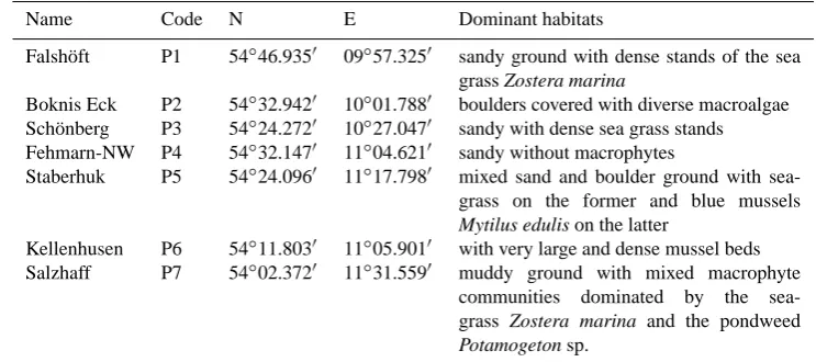
Table 1. Coordinates and habitat characteristics of the stations sampled during this survey.

Name Code N E Dominant habitats

Falsh¨oft P1 54◦46.9350 09◦57.3250 sandy ground with dense stands of the sea grass Zostera marina

Boknis Eck P2 54◦32.9420 10◦01.7880 boulders covered with diverse macroalgae Sch¨onberg P3 54◦24.2720 10◦27.0470 sandy with dense sea grass stands Fehmarn-NW P4 54◦32.1470 11◦04.6210 sandy without macrophytes

Staberhuk P5 54◦24.0960 11◦17.7980 mixed sand and boulder ground with sea-grass on the former and blue mussels Mytilus edulis on the latter

Kellenhusen P6 54◦11.8030 11◦05.9010 with very large and dense mussel beds Salzhaff P7 54◦02.3720 11◦31.5590 muddy ground with mixed macrophyte

communities dominated by the sea-grass Zostera marina and the pondweed Potamogeton sp.

Fig. 1. Chart depicting the position of the seven stations in Kiel and L¨ubeck Bight sampled in this survey.

benthic communities are presumably “natural”, whereas out-side, which they could be, indicative of an anthropogenic sig-nal (e.g. intensifying pollution) or climate change. This zone of confidence will become more reliable when the duration of the monitoring grows. Additionally, we recommend a known statistical procedure, RELATE, to distinguishing between di-rectional shift in time and random temporal fluctuations in community composition. We will discuss the risk of over-looking change if the monitoring phase is started too late (or run for too long) and already includes first shifts in commu-nity structure driven by environmental change.

2 Materials and methods

2.1 Assessment of community variability

2.1.1 Stations

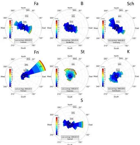
Along the German Baltic Sea coast, in the Kiel and L¨ubeck bights, seven permanent stations were selected for this long-term programme to assess hard-bottom community assem-blage dynamics (Fig. 1). The stations from NW to SE were Falsh¨oft, Boknis Eck, Sch¨onberg, Fehmarn, Staberhuk, Kel-lenhusen and Salzhaff (see Table 1 for site characteristics). Among all stations, only Fehmarn is exposed to the region-ally most frequent strong winds from the SW to the NW. The remaining sites are exposed to the rarer storms from northern or easterly directions. The dominant current directions and speeds are given in Fig. 2.

2.1.2 Deployment of settlement panels

Fig. 2. Distribution of current regimes at the seven stations, averaged over all six years of the survey. Degrees indicate the current directions (by segments of 30◦), percentages give the commonness of a given current direction, the colour coding indicates the average speed of currents in a given directional segment. (A) through (G) are the summer current regimes at the different stations Fa through S.

2.1.3 Characterization of communities

In the lab, the various components of the communities were identified to the lowest possible taxonomic level (species or genus), and their relative cover on the panel was estimated to the nearest 5 %. Additionally, each genus or species was at-tributed to a functional group defined by the adult properties with regard to size, growth form, trophic type and modularity.

Table 2. Functional traits used for grouping. The metrics used are considered ecologically relevant and they can be surrogates for other traits. Thus, body size correlates closely with longevity or metabolic rate, growth form determines the species’ strategy for exploiting resources such as substratum or light, etc. Ecosystem services associated with these and similar traits are discussed in Bremner et al. (2006) and Wahl (2009).

Adult body size Growth form Trophic type Modularity

S<1 mm E encrusting A autotroph S solitary M 1–10 mm M massive P predator C colonial L 10–100 mm B bushy S suspension feeder

XL 100–1000 mm F filamentous D deposit feeder XXL>1000 mm G grazer

should be noted that this functional characterization applies to the adult stage only.

Subsequently all organisms were scraped off the panel and dried to constant weight at 60◦C to obtain the community dry weight, then burned at 500◦C for 24 h to obtain the commu-nity ash weight.

Species or genus identity as well as relative abundance were used to describe and analyse the compositional proper-ties of a panel community. Dry weight (DW) and ash free dry weight (AFDW) were obtained to describe the panel commu-nities’ productivity as biomass accumulation over 12 months. While community composition was assessed only on the up-ward facing side of the panel to also include all primary pro-ducers, biomass was recorded from both panel sides and was standardized per 100 cm2.

2.1.4 Statistics for community analysis

Data processing: the majority of analyses presented in this study, except the assessment of community biomass, were exclusively performed on the biota that established on the upward facing surface of the settlement panels. Furthermore, we only considered sessile and hemi-sessile (such as tube-dwelling gammarids of the genus Corophium) species and ignored all components of the associated motile fauna, which were not part of a fouling (“attached”) community sensu stricto and that are not being caught quantitatively in the zi-plock bags used for sampling. Since not all of the organisms encountered on the panels could be identified on the species level, the genus was used as the level of taxonomic resolution for all analyses.

Data analyses: correlations between single variables were either Pearson’s (if data were normal) or Spearman’s rank (if data were not normal) correlations. All multivariate analyses were done with the PRIMER (Plymouth Routines in Mul-tivariate Ecological Research) 6.0 software package (Clarke and Warwick, 2007; Clarke and Gorley, 2006). We used prin-cipal component analysis (PCA) to identify the most relevant species, i.e. those that were responsible for the bigger part of the temporal and spatial variation in community structure

during the observation period. For this, only genera which showed ≥10 % cover on at least one of the sampled set-tlement panels were selected. PCA was performed on the untransformed data with a maximum of 5 principal compo-nents. We tested for linear relationships between variables using pair plots prior to this analysis and found no tight, non-linear correlation between any of the species.

To assess the temporal (year to year) dynamics in com-munity composition at the seven study sites, we calculated either the similarity (for the MDS plots) or the dissimilarity (for the variability graphs and the SIMPER (similarity per-centage) analysis) between assemblages that established at the same location in different years. For this, species abun-dance data were averaged across all 8 replicates that were sampled at each site in 1 yr, and then the Bray–Curtis (dis-) similarity for all of the 35 possible pairings (7 sites, 6 yr(dis-) was calculated on the basis of these data. In order to de-scribe a confidence interval of “natural” interannual dissim-ilarity in community structure at a given site, we calculated the mean dissimilarity between communities of yearx and of yearyat a given site. Then we calculated the average and 95 % confidence interval of dissimilarity between commu-nities of 2 different years at this site over the entire moni-toring period. This provided us with the information about the mean and spread (CI) of interannual fluctuations in com-munity composition for all the monitoring sites over all the monitoring period. We proceeded in an analogous manner for the average and CI in the functional composition of com-munities. We also tested for the presence of a serial pattern in community change over time (directional shift) using the RELATE procedure in PRIMER (Clarke and Gorley, 2006; Clarke and Warwick, 2007). For these analyses, data were not transformed nor standardized. SIMPER analyses quan-tified the contributions of single species to the dissimilarity between a given pair of communities.

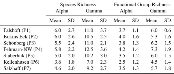
Table 3. Taxonomic and functional richness at the 7 stations: alpha richness is the mean number of taxa or functional groups per panel, gamma richness is the total number of taxa or functional groups found on all panels of a given station (averaged over the years). SD: standard deviation.

Species Richness Functional Group Richness

Alpha Gamma Alpha Gamma

Mean SD Mean SD Mean SD Mean SD

Falsh¨oft (P1) 6.0 2.7 11.0 3.7 3.7 1.1 6.0 0.6

Boknis Eck (P2) 6.0 2.6 10.5 2.5 4.0 1.6 5.3 1.6 Sch¨onberg (P3) 5.5 2.4 11.0 2.1 3.8 1.3 6.2 1.5 Fehmarn-NW (P4) 5.8 2.2 12.5 3.6 4.2 1.4 7.3 1.9

Staberhuk (P5) 5.0 2.0 10.2 3.0 3.5 1.2 6.0 1.5

Kellenhusen (P6) 3.6 1.8 7.0 2.3 2.5 1.2 4.5 1.4

Salzhaff (P7) 4.6 2.0 9.2 2.7 3.5 1.3 5.7 1.8

2.2 Environmental variability

2.2.1 Hydrodynamic model

To provide habitat information in terms of temperature, salin-ity and ocean currents, a comprehensive database was created containing the temporal development of the hydrographic conditions at each of the individual stations (Fig. 1). For this purpose, a three-dimensional hydrodynamic model was used to simulate the hydrographic conditions and their vari-ations in space and time (Kiel Baltic Sea Ice–Ocean Model-BSIOM; Lehmann and Hinrichsen, 2000; Lehmann et al., 2002). The model domain comprises the entire Baltic Sea including the Gulf of Bothnia, Gulf of Finland, Gulf of Riga as well as the Belt Sea, Kattegat and Skagerrak. The hori-zontal resolution of the coupled sea ice–ocean model is at present 2.5 km, with 60 vertical levels specified. The cou-pled sea ice–ocean model is forced by realistic atmospheric conditions taken from the Swedish Meteorological and Hy-drological Institute (SMHI Norrk¨oping, Sweden) meteoro-logical database (L. Meuller, personal communication, 2003) which covers the whole Baltic drainage basin on a regu-lar grid of 1◦×1◦with a temporal increment of 3 h. The database consists of synoptic measurements interpolated on the regular grid by using a 2-D uni-variate optimum interpo-lation scheme. This database, which for modelling purposes is further interpolated onto the model grid, includes surface pressure, precipitation, cloudiness, air temperature and wa-ter vapour mixing ratio at 2 m height and geostrophic wind. Wind speed and wind direction at 10 m height are calculated from geostrophic winds in consideration of different rough-ness on the open sea and near the coastal area (Bumke et al., 1998). Forcing functions of BSIOM such as wind stress, ra-diation and heat fluxes were calculated according to Rudolph and Lehmann (2006). Physical properties simulated by the hydrodynamic model agree well with known circulation fea-tures and observed physical conditions in the Baltic Sea (e.g. Hinrichsen et al., 1997; and Lehmann et al., 2012).

2.2.2 Drift model

Simulated three-dimensional velocity fields were extracted from daily mean property fields provided by the hydrody-namic model in order to develop a database for particle track-ing. This data set offers the possibility to derive Lagrangian drift routes by calculating the advection of “marked” wa-ter particles through space and time. The three-dimensional trajectories of the simulated drifters were computed using a 4th order Runge–Kutta scheme (Hinrichsen et al., 1997). In order to consider the particle drift in relation to its spa-tial and temporal variability, particles were seeded for the time period 2005–2009 at the panel locations every 5 days from 1 July to 30 August, resulting in 13 different release dates. The latter is based on the duration of the maximum dispersal and recruitment of many locally abundant species (Thomsen et al., 2010).

The experimental design required the determination of the origins of individual particles which settled during the prime settlement period (late May to August, Thomsen et al., 2010) at the panel positions (Fig. 1). Thus, particles were inserted into the simulated flow fields at the sea sur-face at the different panel positions and their drift was back calculated for a 40 days drift period. For each of the dif-ferent particle release dates, 175 drifters were seeded on a regular spaced grid around the panel positions. The em-ployed particle tracking technique allowed backward calcu-lation of drift trajectories by simply reversing the temporal sequence of the three-dimensional flow fields and by invert-ing the sign of the horizontal components of the velocity vec-tor (Hinrichsen et al., 1997).

2.2.3 Statistical parameters of original particle distributions

characterisation of the back-calculated starting positions of the particles was performed by the calculation of statistical parameters including PCA. In our case, PCA has been used in a simple direction to determine the first two principle compo-nents from a bivariate data set with latitudes and longitudes of the starting positions of the particles. The spatial extension and density of the starting positions of the particles is defined as the dispersal kernel (Edwards et al., 2007). By using this approach, we have quantitatively estimated the extension of the particle release area by calculating their dispersal kernels (Edwards et al., 2007) in terms of variance ellipses. The cal-culation is based on the variance of the spatial components (longitudes and latitudes of the starting positions of the par-ticles) as well as on their covariance. The latter enables us to find a principle angle describing the variations of parti-cles around a mean position along a set of directions other than those of the longitudinal and latitudinal axis of the parti-cle distributions (Preisendorfer, 1988). The dispersal kernels were found to be Gaussian in form, and similar to Edwards et al., (2007) we calculated four parameters: (1) the mean of the starting positions of particles, (2) the major and (3) minor axis of variability of the spatial starting positions of particles and (4) the principal angle of the orientation of the major axis. The identification of the dispersal scale (extension of the particle distribution) is given by the size of the variance ellipse as calculated from the major and minor axes sizes.

Variability of the sea surface environmental variables such as current direction, current velocity, salinity and tempera-ture were quantified as the mean Bray–Curtis dissimilarities between consecutive years.

2.2.4 Relation between hydrographical and compositional variability

For the assessment of the influence of the interannual vari-ability in hydrographical conditions (see below) during the period of maximum recruitment (June to August) on the in-terannual variability in community composition the oceano-graphic variables used were the June-July-August-averages in sea surface salinity, temperature, current velocity and current direction at each station. Main current velocities and directions were site dependent, thus the recruitment depends not only on the interannual variability of the at-mospheric conditions but also on the site characteristics (Fig. 1). Histograms of daily surface velocities distributed over 30◦_{-segment velocity directions were extracted from} BSIOM for the period 2005–2010 (Fig. 2). Those sites where the flow is of retentive character show small current ve-locities and nearly equal distribution of current directions (e.g. B and K); those which are of dispersive character show stronger current velocities and specific current direc-tions (e.g. Sch and Fn). It should be noted that for Salzhaff, currents would most probably be overestimated because of the limited model resolution. Biological, i.e. differences in species abundances, as well as oceanographic

dissimilari-Fig. 3. Dispersal kernels describing the back-calculated origins of drifting particles released at the different platform locations (black dots), 1st to 7th Rows represent the locations FA = Falsh¨oft, B = Boknis Eck, Sch = Sch¨onberg, Fn = Fehmarn, St = Staberhuk, K = Kellenhusen, and S = Salzhaff.

ties, i.e. differences in salinity, temperature, current velocity and direction, between consecutive years were calculated for each site using PRIMER. Moreover, to come to one value for the oceanographic variables, the observed dissimilarities (all in %) were averaged across all four of them. Biological and the averaged oceanographic dissimilarities between two consecutive years then formed the statistical pairs that were analysed graphically and by simple linear regression.

3 Results

3.1 Site characteristics

Fig. 4. Confidence intervals of richness in species and in func-tional groups at the panel (alpha diversity) and station level (gamma diversity). Here and elsewhere: B, Boknis Eck; Fa, Falsh¨oft; Fn, Fehmarn; K, Kellenhusen; S, Salzhaff; Sch, Sch¨onberg; St, Staber-huk.

and orientations of the variance ellipses indicate interan-nual variability of the potential backward-calculated origins of drifters as well variations among stations (Fig. 3). The largest horizontal extensions (ellipse area sizes) for most of the drifter origins occurred for the years 2006 and 2007, while the extensions in other years (2005, 2008 and 2009) are relatively small. Marked differences in drift patterns can be recognized when comparisons are made between simulations for the different stations. For the panel locations Falsh¨oft, Boknis, Kellenhusen and Salzhaff, all drifters tended to orig-inate from areas relatively small in size, indicating a gen-eral dominance of retention, i.e. the origin of particles were located relatively close to their final panel positions. The variance ellipses of the most north-western station Falshoeft yielded the highest variation in north–south direction, while for the stations Boknis to Staberhuk the orientation of the ellipses indicates extension of backward-calculated origin of drifters mainly varying in east–west direction. Different patterns emerged for the location Sch¨onberg to Staberhuk, which could be characterized by dispersal. These locations are probably influenced to a higher degree by particles origi-nating in the L¨ubeck and Mecklenburg Bight as well as in the Arkona Basin, likely as a consequence of currents induced by prevailing weak to moderate winds of eastern direction. Ob-viously, largest drift distances were obtained for those time periods and locations, when the stations were located outside the variance ellipses. The latter was mainly observed in 2006 at stations located east of 10◦E.

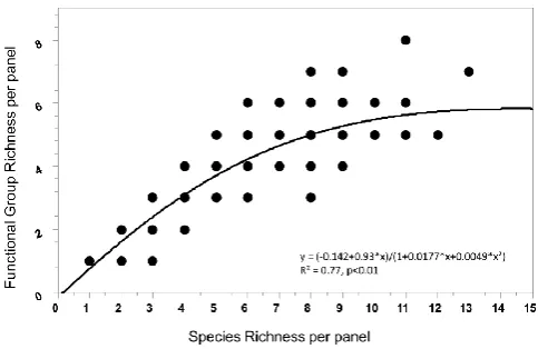
Fig. 5. Relation between species richness and functional group rich-ness at the level of panels. Functional group richrich-ness shows satu-ration at elevated taxonomic richness indicating functional redun-dancy in diverse communities. Note that single dots may represent several replicates andn=277 panels.

3.2 Community traits

3.2.1 Taxonomic and functional composition

Fig. 6. Mean cover (%) of the more common species at the 7 stations and in the 6 yr of surveillance. Station dots connected by lines at the base of the graph do not differ significantly in community composition.

Fig. 7. Mean yearly productivity at the various stations expressed as ash free dry weight (AFDW) accrual per 100 cm2and year.

the genus Polysiphonia as the ones that contributed most to temporal and spatial variability in community structure.

The 60 observed taxa belonged to 15 functional groups (as used in this study). Overall, 16 species were large, 28 medium and 16 small. A filamentous growth form was real-ized by 29 species, a massive growth by 25 and an encrusting

growth by 6 species. 24 algal species and 26 animal species were assessed, of which 50 were solitary and 10 colonial. All of the animal species were suspension feeders since only sessile species were taken into account.

Within 1 yr of recruitment, the upper sides of the pan-els were, on average, covered to between 57 % (±11.3 % SE) in Staberhuk and 103 % (±10 % SE) in Kellenhusen. The two sites east of the isle of Fehmarn (Kellenhusen, Salzhaff) showed generally more cover than the sites on Fehmarn (Fehmarn, Staberhuk) and west of it (Falsh¨oft, Bok-nis Eck, Sch¨onberg, data not shown). Productivity expressed as accrual of ash free dry weight (AFDW) over 12 months tended to increase from NW to SE with the exception of the western-most site, Falsh¨oft, were it was intermediate (Fig. 7). Lowest productivity was found in Boknis Eck and highest in Salzhaff with 0.39 (±0.05 SE) and 2.46 (±0.76 SE) g AFDW 100 cm−2yr−1, respectively. At the 3 western most stations Falsh¨oft, Boknis Eck and Sch¨onberg community productivity was realized to almost equal parts by hetero-and autotrophs, but south-eastward from Fehmarn the contri-bution of heterotrophs continuously increased to reach over 90 % in Salzhaff (Fig. 8). The production of AFDW corre-lated positively with the relative abundance of heterotrophs

Fig. 8. Mean relative contribution of macroalgae (autotrophs) and sessile animals (heterotrophs) to the total annual productivity (% cover per panel) of a panel community (averaged over all panels and years for each station).

3.2.2 Interannual variability in community structure

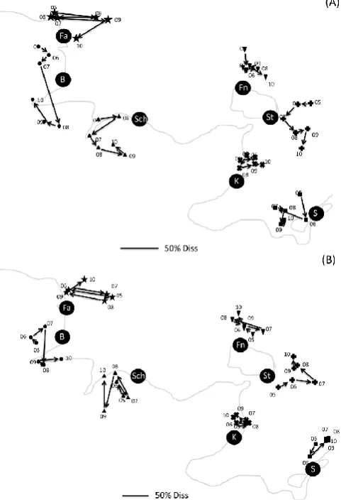
The communities that assembled on the panels of a given station over 12 months differed between consecutive years by 30 to 75 % (Bray–Curtis dissimilarity based on genera richness). At most stations the interannual shifts in commu-nity structure (or function) do not seem to follow a direc-tional trajectory, i.e. their dissimilarity to the initial struc-ture in 2005 did not increase over time (Fig. 9a, b). In Kel-lenhusen the community composition was most stable over time. In Falsh¨oft, Sch¨onberg, Fehmarn and Salzhaff commu-nity composition seems to move randomly around some vir-tual centre. In contrast to this, a tendency towards a direc-tional shift might be detected in Boknis Eck and Staberhuk (Fig. 9a). However, according to the RELATE procedure we employed to detect directional change in community struc-ture over time, none of the trajectories shown in Fig. 9a, including Boknis Eck and Staberhuk, showed a significant temporal seriation. Falsh¨oft seems to oscillate between a Dasya-dominated and a Mytilus-dominated status (Figs. 6, 9a). Boknis Eck shifted from a Cladophora/Ceramium com-munity via a Corophium comcom-munity towards a Hilden-brandia/Polydora community. Sch¨onberg moved from a Ce-ramium/Amphibalanus community via a Ceramium/Mytilus status towards a Corophium/Ceramium community. Fehmarn was in almost all years dominated by Polysiphonia and Amphibalanus, while communities in Staberhuk and Kel-lenhusen were always shaped by Mytilus. Only in Staber-huk we observed a shift in sub-dominant species from Ce-ramium over Amphibalanus to Electra. Salzhaff started as a Mytilus/Amphibalanus community, showed an intermedi-ate status with much Ceramium, Polydora and Corophium besides the dominant Mytilus and featured an even more marked Mytilus dominance with associated Electra in the last years (Figs. 6, 9a). Repeating the analysis with Bray–Curtis

Fig. 9. MDS trajectories between consecutive years for taxonomic (A) and functional (B) composition of the panel communities. The station codes (Fa–S) are placed on the approximate position of the site relative to the coast line in light grey. Within, but not between, compositional categories (species (A), functional groups (B)) are all plots drawn to scale, i.e. same lengths and directions of trajec-tories correspond to an equivalent amount of dissimilarity between consecutive years. A scale bar indicating the 50 % dissimilarity dis-tance is given in each plot.

dissimilarity based on functional richness reveals similar pat-terns for the different stations (Fig. 9b) and again no indi-cation for a significant directional change over time at any of the stations was detectable by RELATE. The shift pat-terns in taxonomic and functional composition of the com-munities behave quite similarly since the respective rho val-ues of the RELATE analyses correlate positively (R2=0.77,

p <0.01).

Fig. 10. 95 % confidence intervals of interannual variability in taxo-nomic (dark grey bars) and functional composition (light grey bars). The confidence interval defines the zone of interannual variabil-ity considered the natural background “noise” (based on the 6 yr surveillance).

analysis): Mytilus edulis (14 %), Amphibalanus improvisus (11 %), Ceramium spp. (11 %), Polysiphonia spp. (8 %), Polydora ciliata (7 %), Callithamnion sp. (6 %), Corophium volutator (6 %), Hildenbrandia rubra (5 %), and Dasya bail-louviana (4 %). The compositional variability pattern was closely matched by a similar pattern in the variability of functional groups (Fig. 10). However, the most important functional traits (medium to large body size for biomass ac-crual and longevity; autotrophy for primary production; sus-pension feeding for pelago-benthic coupling, see Frid et al., 2008) were almost always represented redundantly in a panel community. Medium to large forms are represented by at least one species in all 277 communities, and redundantly so (by 2 or more species) in 98 % of these communities. Sus-pension feeding is represented by at least one species in 97 % of the communities and redundantly so in over 80 % of these. Autotrophy is represented by at least one species in 90 % of the communities and redundantly so in 72 % of these.

3.3 Potential drivers of compositional variability

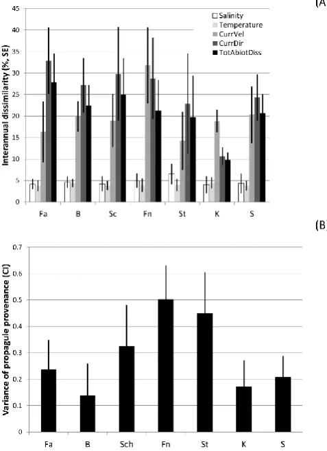
Total abiotic variability (i.e. Bray–Curtis dissimilarities of environmental data) between consecutive years tended to be higher in the western as compared to the eastern part of the range assessed (Fig. 11a) This was mainly due to differences in the variability of the current regime since salinity and tem-perature were quite similar in time (less than 7 and 5 % dis-similarity between consecutive years). The modelled area of provenance of the propagules (Fig. 11b), i.e. the variance el-lipse area sizes (see Fig. 3) representing the variability of current directions weighted by their velocity vector sizes, was most variable in the centre of the geographical range, i.e. around the island of Fehmarn (sites Fn and St) (Figs. 3, 11b). The mean abiotic dissimilarity between the summer months (June–August) of consecutive years (mean of the Bray–Curtis dissimilarities in current direction and

veloc-Fig. 11. (A) Mean dissimilarity between consecutive years in salinity, temperature, current velocity (CurrVel), current direc-tion (CurrDir) and of all these four variables together (TotAbiot-Diss) averaged over the months of June, July, August and over the 6 yr of surveillance. (B) Variance of the propagule origin (area of the dispersal kernels of Fig.3) averaged over the 6 yr of surveillance (with CI).

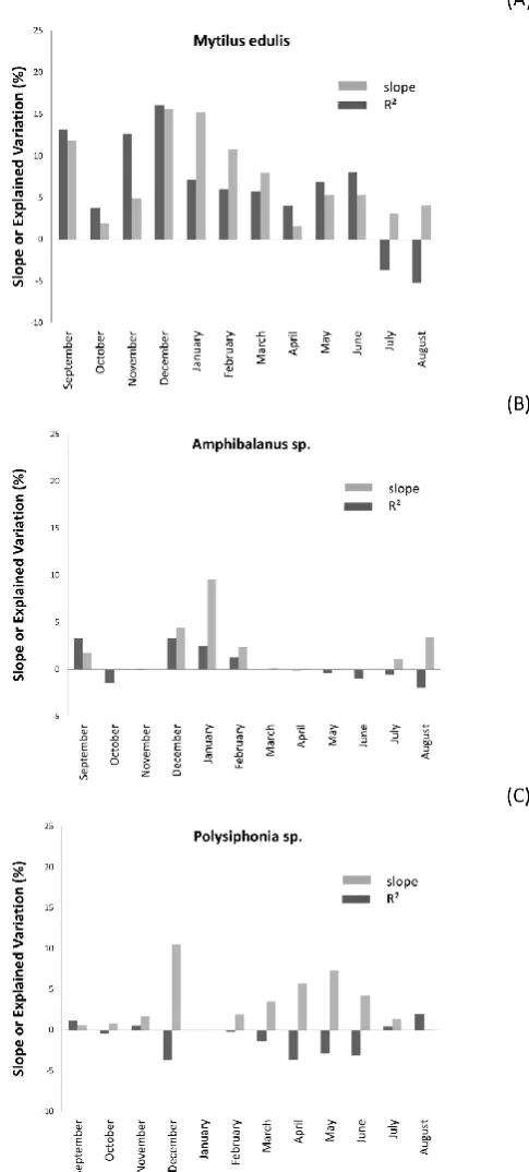
ity, salinity and temperature) correlated positively with the biotic dissimilarity between consecutive years (Bray–Curtis dissimilarity of species composition) (Fig. 12). However, due to the large variance, especially of the abiotic variables, this relationship was only marginally significant (p=0.057), but abiotic variance explained about 55 % of biotic variance.

Fig. 12. Relationships (marginally significant) between taxonomi-cal dissimilarity of communities between consecutive years and the dissimilarity of hydrographical conditions (direction and velocity of currents, salinity, temperature) among the same pairs of years.

Monthly mean salinity did not substantially affect the 3 target species, which drove the bulk of the biotic dissimilarity among consecutive years.

4 Discussion

We found that along the German Baltic coasts of Kiel Bight and L¨ubeck Bight the richness in both, species and functional groups, decreased slightly along the gradient of decreasing salinity (from NW to SE). Additionally, the relative abun-dance of heterotrophs (mostly Mytilus) increased in the same direction, what was accompanied by an increase of annual biomass production and a decrease of interannual variability of community composition. Much of this variance was found to be due to abundance changes of a few “driver” species, mainly Mytilus, Amphibalanus and Polysiphonia.

The abiotic variables with potentially the most impor-tant influence on recruitment and successional dynamics of shallow-water hard-bottom communities in the region we monitored are temperature, salinity, and current regime (e.g. Harley et al., 2006). pH as well as its shifts and fluctuations do not seem to have a major impact on Baltic biota (e.g. Havenhand, 2012). Temperature has effects on the physio-logical rates of adults, larvae and recruits as well as on phe-nology (e.g. Harley et al., 2006; O’Connor, 2007, Gardner et al., 2011; and Sommer et al., 2012). Salinity is a major structuring factor in the Baltic in general and also correlates closely with various community properties (e.g. composi-tion, diversity, and productivity) (e.g. Ojaveer, 2010). Direc-tion and velocity of currents are paramount for the transport of water masses, prey and propagules (e.g. BACC Author Group, 2008).The mean year-to-year dissimilarity of hydro-graphical summer conditions, i.e. current direction and ve-locity, SST (sea surface temperature) and salinity at the dif-ferent stations from June to August, related positively to the

dissimilarity between years in the composition of communi-ties. Abiotic variability explained 55 % of the biological vari-ability found during the five years of monitoring. However, breaking down “abiotic variability” into its components pro-duced a diverse picture: salinity dissimilarity between con-secutive years, which was on average between 4 and 6 %, did not contribute to the compositional dissimilarities measured. Long-term fluctuations in salinity, presumably, represented a minor stress to all those species which were primarily re-sponsible for compositional variability, because none of them is, in the western Baltic, close to its lower salinity tolerance limit (e.g. Bonsdorff, 2006; and Schubert et al., 2011). All of these species occur at all stations that we sampled in the Kiel and L¨ubeck bights which are dissimilar with regard to salinity by up to 22 %. In contrast to this, temperature did affect the abundance of the aforementioned “driver” species which cause most of the structural change among consecu-tive years. The most common autotroph, Polysiphonia, for example, seemed to suffer from warm summers. For the time being, we do not know whether reproduction, growth or physiological performance of the algae were directly af-fected by warm conditions or whether detrimental interac-tions with parasites, pathogens, foulers, competitors or con-sumers intensified under warmer conditions (e.g. Harley et al., 2006; and Wahl et al., 2011b). Furthermore, the dominant heterotrophs, Amphibalanus and – particularly so – Mytilus, benefitted from warm winters. These species settle mainly in summer (June through August) and their larva are released 3–4 weeks prior to settlement. Hence, warmer winter temper-atures might rather enhance the reproductive success of the parent population. At first glance this seems counterintuitive: warm winter temperatures should be stressful since they in-crease the metabolic rate of poikilotherms in times of low planktonic food availability. However, a warmer winter could also lead to earlier spring blooms (if not consumed by over-wintering zooplankton; Sommer and Lewandowska, 2011) improving the food availability for mussels and barnacles in spring/early summer, i.e. when gonads maturate, gametes are released and larvae develop. The causal chain between mild winter temperatures and enhanced mussel and barnacle re-cruitment in the following may be indirect and tortuous – if it is not just a correlated covariance.

Interannual dissimilarity in the taxonomic composition of communities was closely followed by a dissimilarity in the composition of functional groups (r2=0.87,p=0.001). In this approach functional groups are defined by the combina-tion of 4 funccombina-tional traits describing a species’ properties at the adult stage with regard to body size, growth form, trophic type and modularity. A difference in only one of these traits is sufficient to classify two functional groups as distinct in our analysis of dissimilarity. This linkage is justified if we assume that it makes a difference whether suspension feed-ing is carried out by a large, branchfeed-ing and colonial organ-ism or a medium sized, solitary organorgan-ism of massive growth form. The body size of solitary organisms has been regarded

as a proxy for longevity and an indication of low metabolic rates, while growth form may determine competitiveness for resources including light and substratum (e.g. Woodward et al., 2005; Hillebrand, 2004; and Micheli and Halpern, 2005). When, however, we focus on the absence or presence of a certain service (e.g. bentho-pelagic coupling, primary pro-duction, and habitat engineering) in the community we may consider the traits singly, i.e. disregarding the other three traits of its bearer. Under this perspective, the substantial in-terannual variability in the composition of functional groups is not accompanied by a similar variability in the combina-tion of ecological traits in the communities. In fact, essential services like primary production, suspension feeding or pro-vision of structure were provided by at least one species in nearly all communities and by more than one species (i.e. redundantly) in the great majority of communities. Thus, as a general rule that follows from our analyses, despite a sub-stantial interannual variability in functional group composi-tion, the essential services of the shallow-water hard-bottom communities in the western Baltic were warranted. It should be noted at this point that by exclusively considering the ses-sile components of the assemblages on the settlement panels, the trophic diversity of animals was essentially reduced to one trait: suspension feeding.

Increased taxa diversity could strengthen the stability of community services because functional group richness ap-proaches saturation in very taxa-rich communities. This pat-tern suggests that the more taxa rich a community is the higher is the probability that a functional group and, even more so, single functional traits are represented by more than one species. Consequently, the loss of a species will not au-tomatically be accompanied by the loss of a function. This aspect of stability (“insurance hypothesis”) cannot, however, be related directly to the interannual dissimilarity quantified here because each year the communities recruited anew from the meta-community of the region and without direct link to the previous year’s panel community at a given site.

under variable abiotic conditions. It was postulated earlier that taxonomic diversity favours resistance to environmental change in functionally poor but not in functionally rich sys-tems (Wahl et al., 2011a). This hypothesis, however, cannot be examined here, because the regions did not differ enough with regard to functional diversity.

In this study we have pursued a double aim: we attempted to quantify the temporal “noise” in the composition of one-year old western Baltic hard-bottom communities, and we tried to identify some possible causes for the observed biotic variability. While the study has some strengths it also fea-tures certain limitations. Here we consider as strong points that the quantification of compositional variability was not confounded by community age, spatial variability, substra-tum type, sampling procedure, or season, all of which were kept constant. On the other hand, the recruitment and suc-cession process was arrested at the age of 12 months and the interannual dissimilarity of communities could diverge or converge thereafter. Another limitation is that we only as-sessed sedentary species and ignored the variability of motile consumers. A further weakness will certainly decrease with the continuation of this project: while one of our major goals was to distinguish noise (natural fluctuations) from the sig-nal of global change (directiosig-nal shifts), we cannot be sure whether the signal is not already included in the noise. A sig-nal would be detectable by an MDS trajectory (such as those shown in Fig. 9) over time that does not return to previous points. At this point in time, in only two cases, i.e. Boknis Eck and Staberhuk, we observed that the youngest point is furthest away from the oldest. It is well known, however, that climate change is overlain by local fluctuations and decadal oscillations (e.g. Parker et al., 2007; and Frid, 2011) and it is therefore advisable to assess communities’ compositional variability on a decadal scale before tempting to quantify the range of “natural” background variability as the ecological noise. Also, this should only be undertaken, if the MDS tra-jectory does not indicate a tendency for directional change. Furthermore, the western Baltic Sea, the transition zone be-tween brackish Baltic and saline North Sea waters, is known as an area of very high variability of oceanographic condi-tions (very noisy). Further to the east, in the Baltic roper, hy-drographical conditions are more stable (less noisy) so that directional shifts due to climate change would be easier to detect. These points in mind, our results about natural noise in the composition of western Baltic hard-bottom communi-ties should be considered with some caution while the ongo-ing program continuously solidifies this knowledge base.

The noise, i.e. the dissimilarity of community composi-tions between years, decreases from NW to SE along the de-creasing diversity gradient and with the inde-creasing relative abundance of heterotrophic organisms. While in Kiel Bight proper (stations Fa, B, Sch) the communities vary struc-turally by, on average, 80 % between years, this variability averages around only 55 % in L¨ubeck Bight proper (stations K and S). In addition, the confidence intervals of the

inter-annual fluctuations cover the range between 75 and 93 % in Kiel Bight and between 45 and 65 % in L¨ubeck Bight. We assume that this apparently higher stability of community structure in the eastern stations is caused by reduced abiotic variability and the high relative abundance of the competi-tively extremely dominant mussel Mytilus edulis. A signal for a severe disturbance or a regime shift might be identi-fied when the composition of communities recruited under the conditions described here leaves this confidence interval. Such a signal could be detected more easily in the less fluctu-ating communities of the eastern part of the salinity gradient studied here. Directional shift over time which might signal a change driven by climate change can be distinguished from a more random oscillation of community structure (or func-tional composition) using the RELATE procedure. This tool may prove useful to detect climate change signals when a time series of biological samples covering a decade or more is available. The close correlation between taxonomic and functional rhos in the RELATE analyses seems to indicate that any shift in species composition is associated with a shift in functional group composition. This is probably due to low redundancy of functional groups in this species-poor system. However, a shift in functional group composition is not necessarily associated with a loss (or gain) of functional traits or services in the community, as discussed above, but it bears the potential for such a loss or gain. It remains to be investigated whether RELATE is restricted to the detec-tion of steady change in community composidetec-tion or commu-nity functioning, and whether more abrupt shifts, i.e. abrupt regime shifts jeopardize its suitability.

We conclude that along the German Baltic coast of the Kiel and L¨ubeck bights the relative abundance of het-erotrophs increases, annual productivity (biomass increment) tends to increase, and compositional variability in time tends to decrease. A substantial part of interannual compositional dissimilarity is driven by the variability of environmental conditions such as the current regime in summer and the tem-peratures in winter. Both of these are expected to change in the coming decades (BACC Author Group, 2008).

Acknowledgements. We greatly appreciate Renate Schuett’s metic-ulous identification and quantification of the panel communities.

The service charges for this open access publication have been covered by a Research Centre of the Helmholtz Association.

Edited by: H. Bange

References

BACC Author Group: Assessment of climate change for the Baltic Sea Basin, Springer, 2008.

Bonsdorff, E.: Zoobenthic diversity-gradients in the Baltic Sea: Continuous post-glacial succession in a stressed ecosystem, J. Exp. Mar. Biol. Ecol., 330, 383–391, 2006.

Bremner, J., Rogers, S. I., and Frid, C. L. J.: Matching biological traits to environmental conditions in marine benthic ecosystems, J. Mar. Syst., 60, 302–316, 2006a.

Bremner, J., Rogers, S. I., and Frid, C. L. J.: Methods for describ-ing ecological functiondescrib-ing of marine benthic assemblages usdescrib-ing biological traits analysis (BTA), Ecol. Indic., 6, 609–622, 2006b. Bumke, K., Karger, U., Hasse, L., and Niekamp, K.: Evaporation over the Baltic Sea as an example of a semi-enclosed sea, Contr. Atmos. Phys., 71, 249–261, 1998.

Carr, M., Woodson, C. B., Cheriton, O. M., Malone, D., McManus, M. A., and Raimondi, P. T.: Knowledge through partnerships: in-tegrating marine protected area monitoring and ocean observing systems, Front. Ecol. Environ., 9, 342–350, 2011.

Clarke, K. R. and Gorley, R. N.: PRIMER v6: User Man-ual/Tutorial, PRIMER-E, 2006.

Clarke, K. R. and Warwick, R. M.: Change in Marine Commu-nities: An Approach to Statistical Analysis and Interpretation, PRIMER-E, 2001.

Cowie, J.: Climate change: biological and human impacts, Univer-sity Press Cambridge, 487 pp., ISBN 978-0-521-69619-7, 2007. Edwards, K. P., Hare, J. A., Werner, F. E., and Seim, H.: Using 2-dimensional dispersal kernels to identify the dominant influences on larval dispersal on continental shelves, Mar. Ecol. Prog. Ser., 352, 77–87, 2007.

Firth, L. B. and Hawkins, S. J.: Introductory comments – Global change in marine ecosystems: Patterns, processes and interac-tions with regional and local scale impacts, J. Experim. Mar. Biol. Ecol., 400, 1–6, 2011.

Frid, C. L. J.: Temporal variability in the benthos: Does the sea floor function differently over time, J. Exp. Mar. Biol. Ecol., 400, 99– 107, 2011.

Frid, C. L. J., Buchanan, J. B., and Garwood, P. R.: Variability and stability in benthos:twenty-two years of monitoring off Northum-berland, ICES J. Mar. Sci., 53, 978–980, 1996.

Frid, C. L. J., Paramor, O. A. L., Brockington, S., and Bremner, J.: Incorporating ecological functioning into the designation and management of marine protected areas, Hydrobiologia, 606, 69– 79, 2008.

Gamfeldt, L., Hillebrand, H., and Jonsson, P. R.: Multiple func-tions increase the importance of biodiversity for overall ecosys-tem functioning, Ecology, 89, 1223–1231, 2008.

Gardner, J. L., Peters, A., Kearney, M. R., Joseph, L., and Heinsohn, R.: Declining body size: a third universal response to warming, Trends Ecol. Evol., 26, 285–291, 2011.

Greene, C. H. and Schoener, A.: Succession on marine hard sub-strata – a fixed lottery, Oecologia, 55, 289–297, 1982.

Harley, C. D. G., Hughes, A. R., Hultgren, K. M., Miner, B. G., Sorte, C. J. B., Thornber, C. S., Rodriguez, L. F., Tomanek, L., and Williams, S. L.: The impacts of climate change in coastal marine systems, Ecol. Lett., 9, 228–241, 2006.

Havenhand, J. N.: How will Ocean Acidification Affect Baltic Sea Ecosystems? An Assessment of Plausible Impacts on Key Func-tional Groups, Ambio, 41, 637–644, 2012.

Hillebrand, H.: On the generality of the latitudinal diversity gradi-ent, Am. Nat., 163, 192–211, 2004.

Hinrichsen, H.-H., Lehmann, A., St. John, M. S., and Br¨ugge, B.: Modeling the cod larvae drift in the Bornholm Basin in summer 1994, Cont. Shelf Res., 17, 1765–1784, 1997.

Jackson, A. C. and McIlvenny, J.: Coastal squeeze on rocky shores in northern Scotland and some possible ecological impacts, J. Experim. Mar. Biol. Ecol., 400, 314–321, 2011.

Kordas, R. L., Harley, C. D. G., and O’Connor, M. I.: Community ecology in a warming world: The influence of temperature on in-terspecific interactions in marine systems, J. Experim. Mar. Biol. Ecol., 400, 218–226, 2011.

Lehmann, A. and Hinrichsen, H.-H.: On the thermohaline variabil-ity of the Baltic Sea, J. Mar. Syst., 25, 333–357, 2000.

Lehmann, A., Hinrichsen, H-H., and Krauss, W.: Effects of remote and local atmospheric forcing on circulation and upwelling in the Baltic Sea, Tellus, 54A, 299–316, 2002.

Lehmann, A., Getzlaff, K., and Harlaß, J.: Detailed assessment of climate variability in the Baltic Sea area for the period 1958 to 2009, Climate Res., 46, 185–196, 2011.

Lehmann, A., Myrberg, K., and H¨oflich, K.: A statistical approach to coastal upwelling in the Baltic Sea based on the analysis of satellite data for 1990–2009, Oceanologia, 54, 369–393, 2012. Lockwood, B. L. and Somero, G. N.: Invasive and native blue

mus-sels (genus Mytilus) on the California coast: The role of physi-ology in a biological invasion, J. Experim. Mar. Biol. Ecol., 400, 167–174, 2011

Loreau, M. and de Mazancourt, C.: Species synchrony and its drivers: Neutral and nonneutral community dynamics in fluctu-ating environments, American Naturalist, 172, E48–E66, 2008. McNaughton, S. J.: Diversity and stability of ecological

communi-ties – comment on the role of empiricism in ecology, Am. Nat., 111, 515–525, 1977.

Merzouk, A. and Johnson, L. E.: Kelp distribution in the northwest Atlantic Ocean under a changing climate, Journal of Experimen-tal Marine Biology and Ecology, 400, 90–98, 2011.

Micheli, F. and Halpern, B. S.: Low functional redundancy in coastal marine assemblages, Ecol. Lett., 8, 391–400, 2005. Millennium Ecosystem Assessment: Ecosystems and human

well-being: Synthesis, Island Press, 2005.

O’Connor, M. I., Bruno, J. F., Gaines, S. D., Halpern, B. S., Lester, S. E., Kinlan, B. P., and Weiss, J. M.: Temperature control of lar-val dispersal and the implications for marine ecology, evolution, and conservation, Proc. Natl. Acad. Sci. USA, 104, 1266–1271, 2007.

Ojaveer, H. A., Jaanus, B. R., MacKenzie, G. M., Olenin, S., Radziejewska, T., Telesh, I., Zettler, M. L., and Zaiko, A.: Sta-tus of Biodiversity in the Baltic Sea, Plos One, 5, e12467, doi:10.1371/journal.pone.0012467, 2010.

Parker, D., Folland, C., Scaife, A., Knight, J., Colman, A., Baines, P., and Dong, B. W.: Decadal to multidecadal variability and the climate change background, J. Geophys. Res.-Atmos., 112, D18115, doi:10.1029/2007JD008411, 2007.

Pollack, J. B., Palmer, T. A., and Montagna, P. A.: Long-term trends in the response of benthic macrofauna to climate variability in the Lavaca-Colorado Estuary, Texas, Mar. Ecol. Prog. Ser., 436, 67–80, 2011.

Preisendorfer, R. W.: Principal Component Analysis in Meteorol-ogy and Oceanography, Elsevier Science Publishers BV, New York, 1988.

R Development Core Team R: A language for statistical computing, R Foundation for Statistical Computing, Vienna, Austria, ISBN 3-900051-07-0, http://www.R-project.org, 2010.

Reise, K.: Mosaic cycles in the marine benthos, in: The mosaic-cycle concept of ecosystems, edited by: Remmert, H., Springer, 1991.

Rudolph, C. and Lehmann, A.: A model-measurements compari-son of atmospheric forcing and surface fluxes of the Baltic Sea, Oceanologia, 48, 333–380, 2006.

Schubert, H., Feuerpfeil, P., Marquardt, R., Telesh, I., and Skarlato, S.: Macroalgal diversity along the Baltic Sea salinity gradient challenges Remane’s species-minimum concept, Mar. Poll. Bull., 62, 1948–1956, 2011.

Solan, M., Raffaelli, D. G., Paterson, D. M., White, P. C. L. and Pierce, G. J.: Marine biodiversity and ecosystem function: em-pirical approaches and future research needs – Introduction, Mar. Ecol.-Prog. Ser., 311, 175–178, 2006

Somero, G. N.: The physiology of climate change: how potentials for acclimatization and genetic adaptation will determine “win-ners” and “losers”, J. Exp. Biol., 213, 912–920, 2010.

Sommer, U. and Lewandowska, A.: Climate change and the phyto-plankton spring bloom: warming and overwintering zoophyto-plankton have similar effects on phytoplankton, Glob. Change Biol., 17, 154–162, 2011

Sommer, U., Aberle, N., Lengfellner, K., and Lewandowska, A.: The Baltic Sea spring phytoplankton bloom in a changing cli-mate: an experimental approach, Mar. Biol., 159, 2479–2490, 2012.

Spencer, M., Birchenough, S. N. R., Mieszkowska, N., Robinson, L. A., Simpson, S. D., Burrows, M. T., Capasso, E., Cleall-Harding, P., Crummy, J., Duck, C., Eloire, D., Frost, M., Hall, A. J., Hawkins, S. J., Johns, D. G., Sims, D. W., Smyth, T. J. and Frid, C. L. J.: Temporal change in UK marine communities: trends or regime shifts?, Mar. Ecol. Evolut. Perspec., 32, 10–24, doi:10.1111/j.1439-0485.2010.00422.x, 2011

Thomsen, J., Saph¨orster, J., Heinemann, A., and Melzner, F.: Im-pacts of hypercapnia and temperature on physiological per-formance of marine invertebrates from the Baltic Sea, Comp. Biochem. Phys. A, 153A, S169–S169, 2009.

Thomsen, J., Gutowska, M. A., Saph¨orster, J., Heinemann, A., Tr¨ubenbach, K., Fietzke, J., Hiebenthal, C., Eisenhauer, A., K¨ortzinger, A., Wahl, M., and Melzner, F.: Calcifying inverte-brates succeed in a naturally CO2-rich coastal habitat but are threatened by high levels of future acidification, Biogeosciences, 7, 3879–3891, doi:10.5194/bg-7-3879-2010, 2010.

Valdivia, N. and Molis, M.: Observational evidence of a negative biodiversity-stability relationship in intertidal epibenthic com-munities, Aquat. Biol., 4, 263–271, 2009.

von Bertalanffy, L.: The theory of open systems in physics and bi-ology, Science, 111, 23–29, 1960.

Wahl, M.: Ecological modulation of environmental stress: inter-actions between ultraviolet radiation, epibiotic snail embryos, plants and herbivores, J. Animal Ecol., 77, 549–557, 2008 Wahl, M.: Habitat characteristics and typical functional groups, in:

Marine Hard Bottom Communities: patterns, dynamics, diver-sity, and change, edited by: Wahl, M., Springer, 206, 7–18, 2009 Wahl, M., Link, H., Alexandridis, N., Thomason, J. C., Cifuentes, M., Costello, M. J., da Gama, B. A. P., Hillock, K., Hobday, A. J., Kaufmann, M. J., Keller, S., Kraufvelin, P., Kr¨uger, I., Lauter-bach, L., Antunes, B .L., Molis, M., Nakaoka, M., Nystr¨om, J., Radzi, Z., Stockhausen, B., Thiel, M., Vance, T., Weseloh, A., Whittle, M., Wiesmann, L., Wunderer, L., Yamakita, T., and Lenz, M.: Re-structuring of marine communities exposed environmental change: A global study on the interactive ef-fects of species and functional richness, Plos One, 6, e19514, doi:10.1371/journal.pone.0019514, 2011a.

Wahl, M., Jormalainen, V., Eriksson, B. K., Coyer, J. A., Molis, M., Schubert, H., Dethier, M., Karez, R., Kruse, I., Lenz, M., Pearson, G., Rohde, S., Wikstr¨om, S. A., and Olsen, J. L.: Stress ecology in Fucus: abiotic, biotic and genetic interactions, Adv. Mar. Biol., 59, 37–105, 2011b.

Woodward, G.,Ebenman, B., Emmerson, M., Montoya, J. M., Ole-sen, J. M., Valido, A., and Warren, P. H.: Body size in ecological networks, Trends Ecol. Evol., 20, 402–409, 2005.