34
Wilmott
magazine
The Heston–Hull–White Model Part II:
Numerics and Examples
1 Introduction
This is the second article in a series of three on financial modeling using the Heston-Hull-White model. The aim of this series is to show the full life cycle of model development and implementation.
This article reviews the methods for pricing European options and suggests fast numerical methods for the pricing procedure. In our case we consider the pricing of calls and puts as well as caps and floors using the Carr and Madan (1999) framework. There have been many frameworks suggested in the litera-ture, see for instance Fang and Osterlee (2008), Attari (2004), Lord (2008), Lewis (2000). We review the method of computing stable prices by optimal dampening, see Lord and Kahl (2006). The suggested instruments are liquid traded options and can be used in a calibration procedure. This is a backward problem. We try to infer model parameters from market quotes. Backward problems are known to be unstable but these methods are frequently used to estimate model param-eters. Therefore, we show which algorithms may be used to tackle this problem. Finally, we proceed by considering discretization methods which can then be applied in Monte Carlo simulation to price exotic path dependent payoffs. For the model under consideration we propose to implement a stable numeri-cal scheme based on Andersen (2006). There are several new methods for dis-cretizing a square root dynamic, see for instance Glasserman and Kim (2008), Van Haastrecht (2008) or Chan and Joshi (2010).
For all the algorithms we provide source code which can be obtained by writing to joerg.kienitz(at)gmx.de.
In the third and final article of this series we describe a software frame-work which implements the discussed methods and can be used to apply the Heston-Hull-White model to financial problems. We show how to combine the discussed numerical methods to create a self-contained pricing, hedging and calibration framework.
2 Numerical Methods for Calibration - Fast Fourier
Transform
In this section we compute the characteristic function we use for pricing European options. We review a standard algorithm which we used for pric-ing and calibration purposes. However, we mention some known problems and show how to overcome such problems. This leads to a stable pricing and calibration procedure.
Even though the characteristic function of the Heston–Hull–White model - derived in the first article of the series - is similar to the Heston char-acteristic function, the additional factor requires a significant additional amount of computing time. For example the term
E[Rt,T|Ft]=B(t,T)(rt−ψt)+log
PM(0,t) PM(0,T)
+1
2(V(0,T)−V(0,t))
appearing in calculations includes the market discount curve. Low perform-ance computations however are a bottleneck for a calibration procedure since many computations of the price are necessary.
2.1 The Carr Madan method
Despite the fact that at the time of writing many different methods for computing option prices from the characteristic function exist, for instance Fang and Osterlee (2008) or Lewis (2000), we apply the method introduced in Carr and Madan (1999). It offers the possibility of high performance compu-tations. The idea is to compute the prices for a given maturity but across the whole strike range using a single Fast Fourier Transform. That is of particu-lar importance for pricing with smiles and skews.
By a change of numeraire argument, see for instance Brigo and Mercurio (2006), section 2, the price of a call option is given by
CFt(T,K)=P(t,T)ET
(ST−K)+|Ft
=P(t,T)CT(k)
CT(k)=
∞
k
(exp(s)−exp(k))qT(s)ds (1)
with the log strike price, k = log K. The expectation is taken with respect to the T–forward measure QT. Thus q
T denotes the density of ST with respect to QT conditioned on F
t. In order to apply the FFT the non-discounted price (1) has to be square integrable as a function of k. Since a zero strike implies that the payoff is equal to the forward we see that CT does not tend to zero as k→ −∞. To obtain square integrability Carr and Madan propose to introduce a factor exp(α k), α > 0, and take the Fourier transform with respect to cT(k)=exp(αk)CT(k). One may expect that this function is square integrable for a range of positive values of α. The price below does not analytically depend on α. However, the numerical error that occurs when approximating
Holger Kammeyer
University of Goettingen
Joerg Kienitz
Dt. Postbank AG, e-mail: [email protected]
34-44_Kienitz_Part_II_TP_March_234 34
Wilmott
magazine
35
^
the continuous Fourier transform by the discrete Fast Fourier Transform relies heavily on the choice of α. As an inverse transform (1) is given by
CT(k)=
exp(−αk) 2π
∞
−∞exp(−iuk)ψT(u)du=
exp(−αk) π
∞
0
exp(−iuk)ψT(u)du
with ψT(u)=−∞∞ exp(iuk)cT(k)dk denoting the Fourier transform of cT. The function ψTis related to the T–forward characteristic function φT of ST:|:Ft via the formula:
ψT(u)= φT(u−(α+1)i)
α2+α−u2+i(2α+1)u (2)
Note that α > 0 is also a technical requirement since the FFT algorithm evalu-ates the integrand in zero. The T–forward characteristic function φT can be expressed in terms of the ordinary characteristic function f as follows. By means of Bayes’ rule we have
φT(u)=ET(exp(iuXT)|Ft)
= E(exp(iuXT) dQT
dQ |Ft) E(dQdQT |Ft)
.
For the Radon–Nikodym derivative dQdQT we have
dQT
dQ =
exp(−0Trsds)
P(0,T) =
D(0,T) P(0,T) =
D(0,t)D(t,T) P(0,T) .
Thus, for the Heston–Hull–White model we have
P(t,T)φT(u)=E[D(t,T) exp(iuXT)|Ft]
=E[exp(−Rt,T+iuXT)|Ft] =E[exp(Rt,Ti(u+i)+XHTiu)|Ft] =φR(u+i,t,T)φH(u,t,T)
=:φ˜HHW(u,t,T). (3)
In the above equation, R() again denotes the integrated short rate. We see that using the T–forward measure is very convenient. All discounting issues are done shifting the integration line of the integrated short rate charac-teristic function by one imaginary unit. Now, set ψT as in (2) but substituting φT with ˜f HHW. Then, what we implement as a first step is the following formula
CFt(T,K)=
exp(−αk) π
∞
0
exp(−iuk)ψT(u)du. (4)
The following piece of code gives the implementation:
void FFT::run() {
double SwitchSign, DeltaJ0;
complex<double> IntegrandValue; //integrand value complex<double> EvaluationPoint(0.0, 0.0); //current evaluation point
for(unsigned int j = 0; j < N; j++) //initialize array with integrand values {
SwitchSign = (j % 2) ? (-1.0) : 1.0; //minus one to the power of j
DeltaJ0 = j ? 0.0 : 1.0; //Kronecker-Delta IntegrandValue = itsOption->
Integrand(EvaluationPoint) * SwitchSign * eta;
IntegrandValue *= (1.0 / 3.0) * (3.0 - SwitchSign - DeltaJ0); // correction term
itsOption->PricingArray[2*j] = IntegrandValue.real(); itsOption->PricingArray[2*j+1] = IntegrandValue.imag(); EvaluationPoint += eta; }
// Fast Fourier Transform, see GNU Scientific Library manual
gsl_fft_complex_radix2_forward (itsOption->PricingArray, 1, N); }
There are two points left to remark. The choice of an optimal value of the parameter α and how we approximate the continuous Fourier transform in (4) as precisely as possible using the FFT algorithm. Finally, we show how to price caplets and floorlets in the Hull–White model. Caplets, Cpl, are equiva-lent to zero bond puts, ZBP, via
Cpl(t,t1,t2,N,X)=NZBP(t,t1,t2,X). (5)
Here t denotes the present time (which will be zero in the implementa-tion), t1 and t2 are starting and ending time of the caplet, N is the nominal value and X is the strike interest rate. The modified values X and N are given by
X= 1
1+X(t2−t1)
and N=N(1+X(t2−t1)). (6)
Analogously, we have the formula
Fll(t,t1,t2,N,X)=NZBC(t,t1,t2,X) (7)
which relates floorlets to zero bond calls. This should clarify the source code snippet that computes the caplet or floorlet price.
void HullWhite::CapletFloorlet::run() {
itsCorP = -itsCorF + 1; itsT = itsStartT;
itsBondMaturity = itsEndT;
itsN = itsCapletFloorletN*(1.0 + itsCapletFloorletK* (itsEndT - itsStartT)); itsK = 1.0 / (1.0 + itsCapletFloorletK *
(itsEndT - itsStartT)); HullWhite::ZeroBondOption::run(); }
34-44_Kienitz_Part_II_TP_March_235 35
36
Wilmott
magazine
The function call in the last command line will compute the zerobond option price using a Black–like formula. The availability of such an analytical formula renders the Hull–White calibration very fast with fast meaning almost instantaneously. The final function call is implemented as follows:
void HullWhite::ZeroBondOption::run() {
double P_T = getZeroBondValue(itsT);
double P_S = getZeroBondValue(itsBondMaturity); double sigma_p = itsEta * sqrt((1.0 - exp
(-2.0 * itsLambda * itsT))
/ (2.0 * itsLambda)) * factorB(itsT, itsBond Maturity);
double h = (1.0 / sigma_p) * log (P_S / (P_T * itsK)) + sigma_p / 2.0;
if(itsCorP == 1)
itsPrice = itsN * (P_S * CumulativeNormal(h) - itsK * P_T * CumulativeNormal(h - sigma_p)); else
itsPrice = itsN * (itsK * P_T * CumulativeNormal(-h + sigma_p)
- P_S * CumulativeNormal(-h)); //equation 3.41
setUp2D(true); }
2.2 The optimal damping factor
The auxiliary parameter α has to be chosen within a certain range [αmin, αmax]. This is to guarantee square integrability. Within the allowed range there are inappropriate choices of α which cause the integrand to be highly oscillat-ing and can lead to significant mispricoscillat-ing of standard options. For instance it can lead to negative prices.
Lord and Kahl (2006) analyzed the problem of computing an optimal dampening parameter. Ideally, an optimization algorithm for α minimizes the total variation of the integrand y. This would require more function evaluations than the original problem and thus is mainly useless in prac-tice. Therefore, Lord and Kahl (2006) suggest to minimize the maximal value of the integrand which occurs in zero. They consider
α∗=argmin α∈(0,αmax)|
exp(−αk)ψ(0)|.
(8)
In general αmin will be negative and we assume α > 0 there is only one local minimum of this function within the positive reals. So as long as the initial guess the minimization routine starts from is not too large, the mini-mum will be found without any problems involving the maximal allowed alpha αmax which in general is hard to determine.
The following piece of code implements the optimization suggested in Lord and Kahl (2006). For carrying out the optimization we use the LBFGS optimizer implemented in Bochkanov (2010). This library can be downloaded, see references.
void AlphaOptimization::run() // Computes the optimal alpha
{
const double epsG = 0.001; // constant for optimizer const double epsF = 0.0; // constant for optimizer const double epsX = 0.0; // constant for optimizer const int MaxIts = 100; // constant for optimizer ap::real_1d_array x; // alglib real array
x.setbounds(1,1); // set dimensionality x(1) = 1.5;
ap::integer_1d_array nbd;// alglib int array nbd.setbounds(1,1);
nbd(1) = 1; // range for alpha (only lower bound) ap::real_1d_array lbound;// alglib real array
lbound.setbounds(1,1);
lbound(1) = 0.01; //lower bound of allowed range ap::real_1d_array ubound;// alglib real array
ubound.setbounds(1,1);
ubound(1) = 5.0; //upper bound of allowed range. only needed if nbd = 2.
int info;
// the lbfgs optimizer
lbfgsbminimize(MinFunc, itsOption, 1, 1, x, epsG,
epsF, epsX,
MaxIts, nbd, lbound, ubound, info);
itsOption->setAlpha(x(1)); //optimal alpha is found
}
2.3 FFT approximation of continuous Fourier transforms
The precompiled FFT algorithm we wish to apply is taken from the GNU Scientific Library, GSL (2010). It computes the finite sumxk= N−1
j=0
zjexp
−2π N ijk
(9)
with k ranging from 1 to N. From (9) we expect the computation time to correspond to an ordinary square matrix multiplication, i.e. to be of order O(N2). The FFT algorithm improves this computation time to order N times the sum of the prime factors of N. Thus N is chosen to be a power of two resulting in an O(N log N) performance which is a very considerable improvement.
It is implemented using the function
int gsl_fft_complex_radix2_forward (gsl_complex_packed_
array data,
const size_t stride, const size_t n);
of the GSL (2010) library. The latter is available for free. The integral in (4) has the naive approximation
N−1
j=0
exp(−ijηk)ψ(jη)η (10)
as a Riemann sum from zero to Nh. To compute one single call price we nor-malize the strike K to one. The spot price has to be divided by the strike and
34-44_Kienitz_Part_II_TP_March_236 36
Wilmott
magazine
37
^
then it is inserted into the model equations. The latter has the advantage that (8) simplifies to
α∗=argmin α∈(0,αmax)|ψ
(0)|.
(11)
For the calibration we write spot and strike as multiples of the forward. Thus, the call prices which can be deduced from one single FFT will range around the at–the–money level just like the market prices do. With these scalings the grid of k should be centered in zero and is of fineness
λ=2π
Nη. (12)
The grid thus lies within [− b,b] with b = ___λ2 N = __hπ . Substituting k a −b + uλ with u = 0,…,N −1 we obtain
N−1
j=0
exp
−2π N iju
(−1)jψ(jη)η .
(13)
For accuracy both a small h (reducing discretization errors) and a small λ (reducing interpolation errors) are desirable. But a simultaneous diminish-ment is prevented by the relation
λη= 2π N
because N is not only limited by computation time but also by the maximal possible power of two integer on the working machine. For this reason we apply the Simpson’s rule with a correction factor as in Carr and Madan (1999),
N−1
j=0
exp
−2π N iju
(−1)jψ(jη)η
3(3+(−1) j+1−δj
0). (14)
Note that especially for prices of in–the–money options linear inter-polation between two known prices is not completely wrong. That is why a bit contrary to the values recommended by Carr and Madan (1999) we experienced that choosing h according to the rule h = ___2N 14⋅10−3 works fine in
practice.
3 Monte Carlo Heston–Hull–White pricing
With regard to the model dynamic we observe that each time step on the path of the asset price has to be preceded by a time step resulting from simu-lating the evolution of the variance. To obtain an acceptable computation time we wish to implement a discretization scheme with very small bias. To this end we have modified the Quadratic Exponential scheme introduced in Andersen (2006). Source code in C++ has been presented in Duffy and Kienitz (2009) and a version in Visual Basic can be found in Staunton (2007).
3.1 The drifted Quadratic Exponential Scheme
For the Heston model a discretization scheme has been proposed by Andersen (2006). It discretizes the non–central chi square distributed vari-ance process by a dirac delta with an exponential tail for small values of the
variance and by a squared gaussian random variable for larger values of the variance. Again, it is the simplicity of the Gaussian distribution of the short rate Ornstein Uhlenbeck process that allows us to extend the discretization scheme of Andersen (2006) in a bias–free way to include stochastic interest rates. This is possible by sampling just one additional random number for each path since the integrated short rate at maturity is independent and normally distributed with the known parameters. By the Hull-White decom-position the resulting drift is added to the zero short rate final value of the Heston process. We have
XT=R0,T+ˆXT (15)
where ˆXT is the ordinary QE–scheme as in Andersen (2006), p. 19, equation (33).
There is the common problem with Monte Carlo methods that both variance and short rate can become negative during the simulation process. In case of the Heston variance this is only due to the discretization since a CIR process has almost sure non zero paths. To compute the asset price the square root of the variance is taken. Thus, negative values cause errors. The QE–scheme overcomes this issue. In case of negative short rates resulting from the Hull–White model the discretization is not problematic since no range of definition is exceeded. It can indeed occur that after a time step some negative drift arises. This is a general feature of the Hull–White model and not of the Monte Carlo simulation.
For the implementation of the drifted QE scheme we choose the follow-ing constants with respect to the model parameters:
double gamma1 = 0.5; // see Andersen, section 4.2 double gamma2 = 1.0 - gamma1;
itsConst[0] = -((rho * kappa * vLong) / omega) * itsDeltaT; //K_0 itsConst[1] = gamma1 * itsDeltaT * (kappa * rho /
omega - 0.5) - rho / omega; //K_1
itsConst[2] = gamma2 * itsDeltaT * (kappa * rho / omega - 0.5) + rho / omega; //K_2
itsConst[3] = gamma1 * itsDeltaT * (1 - rho * rho); //K_3
itsConst[4] = gamma2 * itsDeltaT * (1 - rho * rho);
Using these constants we implement the drifted QE scheme. To this end we have implemented a function which takes as an input two arrays of uniformly distributed random variables WI1 and WI2 which are then trans-formed to the desired variates. The following piece of code implements this method:
void HestonHullWhite::MonteCarlo::QE(double WI1, double WI2)
{
// Calculate the solution at time level n+1 in terms of solution at time level n double result[3];
// N.B. This assumes that WI1 and WI2 are uniformly distributed
// 1.Variance - see Andersen’s paper double Psi; // switching parameter
34-44_Kienitz_Part_II_TP_March_237 37
38
Wilmott
magazine
double Psi_C = 1.5; // switching parameter
//Parameters used in for loop double a, b2, p, beta, m, s2, c4;
//This becomes a Gaussian variate in the
for loop.
double GV = 0.0;
double Coeff1 = exp(- itsKappa*itsDeltaT); double Coeff2 = 1.0 - Coeff1;
double Coeff3 = itsOmega * itsOmega / itsKappa;
m = itsVLong + (itsVec[2] - itsVLong) * Coeff1;
s2 = itsVec[2] * Coeff1 * Coeff2 * Coeff3 + 0.5 * itsVLong * Coeff2 * Coeff2
* Coeff3;
// martingale correction is required? Store Psi for each time step
Psi = s2 / (m * m);
//Switching Parameter Psi_C if (Psi <= Psi_C)
{
//V[t+Delta] approximated as non
central chi-square
//with one degree of freedom c4 = 2.0 / Psi;
b2 = max(c4 - 1.0 + sqrt(c4*(c4 -
1.0)),0.0); //eq. (27)
a = m / (1.0 + b2); //eq. (28)
//If martingale correction is
required store a and b2
//for each time step since it is needed for calculation of S(t). GV = (sqrt(b2) + InverseCumulative Normal(WI1));
result[2] = a*(GV*GV); //step c
} else {
//Approximation Density with Dirac mass and exponential tail p = (Psi - 1.0) / (Psi + 1.0); //
eq. (29)
beta = (1-p) / m; // eq. (30) //If martingale correction is
required store p and beta at each //time step since it is required
to calculate S(t)
// eq. (25)
if (WI1 <= p)
result[2] = 0.0; else
result[2] = log((1.0 - p) /
(1.0 - WI1)) / beta;
}
result[1] = itsConst[0] + itsConst[1] * itsVec[2] + itsConst[2] * result[2] + sqrt(itsConst[3] * itsVec[2]
+ itsConst[4] * result[2]) * InverseCumulative Normal(WI2);
itsVec[1] += result[1]; itsVec[2] = result[2]; }
The main part of the code is the implementation of the switch-ing rule as suggested in the original work by A06. The final value
result[1] is a predictor corrector scheme applied to the previously generated values.
Finally, the Monte Carlo estimator can be implemented. It calls the QE
scheme and it is given by:
void HestonHullWhite::MonteCarlo::run() {
setSeed(); //path variables
double SumCallValue = 0.0; double SumPutValue = 0.0; double SumIntegralR = 0.0; double SumDiscountFactor = 0.0;
double WI1, WI2; //uniformly distributed randoms
int seed = (int)time(NULL);// use system time to
produce random seed
MersenneTwister2 mt; // init Mersenne Twister mt.SetSeed(seed); // set the seed
for(int i = 1; i <= itsNSIM; ++i) // loop over
simulations
{
// variables containing current values itsVec[1] = log(itsS); // log of
stock price
itsVec[2] = itsVInst; // variance for(int nt = 1; nt <= itsNT; ++nt) // loop over
time steps
{// get random numbers
WI1 = mt.GetRandomNumber(); WI2 = mt.GetRandomNumber();
QE(WI1, WI2); // Call QE
scheme
}
// Hull White integrated short rate process is
normally distributed
double Z = InverseCumulativeNormal(mt. GetRandomNumber());
34-44_Kienitz_Part_II_TP_March_238 38
Wilmott
magazine
39
^
double IntR = getMeanOfIntegral(itsRInst,
0.0, itsT)
+ sqrt(getVarianceOfIntegral(0.0, itsT)) * Z; // store integrated short rate process as well as
discount factor
SumCallValue += exp(-IntR) * max(0.0, exp(itsVec[1] + IntR) - itsK);
SumPutValue += exp(-IntR) * max(0.0, itsK - exp(itsVec[1] + IntR));
SumIntegralR += IntR;
SumDiscountFactor += exp(-IntR); }
//compute arithmetic means as an estimator of expectations
itsIntegralR = SumIntegralR / itsNSIM;
itsDiscountFactor = SumDiscountFactor / itsNSIM; itsCall = SumCallValue / itsNSIM;
itsPut = SumPutValue / itsNSIM; itsPrice = itsCorP ? itsCall : itsPut;
setUp2D(true); }
The code may be modified such that the seed is an argument. Then, using the same seed anytime the simulation starts the random generator produces the same stream of random numbers. We have chosen the system clock to generate a seed. Therefore, for each run you get different random numbers and therefore different realisations for the Monte Carlo estimator.
This presented piece of code is used to price European call and put options. For valuing path dependent options we have to modify the Monte Carlo simulation by storing all the relevant points in the path itsVec[]. Then, the payoff corresponding to the path dependent option can be evalu-ated.
3.2 Numerical Test
We apply the methods to the following sets of parameters:
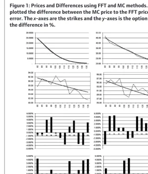
The following results on the one hand show that the prices calculated via FFT and MC agree and therefore we can be sure that both methods are imple-mented correctly. On the other hand we observe that the performance of the MC is worse for long maturities. Table 2 summarizes our findings:
To get a better view on the results we have plotted the outcomes, see figure 1.
The correct mean of discount factors
[image:6.866.383.700.115.723.2]When the number of path simulations is exceeded we just set the element variable itsIntegralR equal to SumIntegralR divided by this number
Table 1: Scenarios for testing the FFT and the MC implementations.
T S0 λ σ t˜ t0 j q v
1 100 0.4 0.2 0.02 0.03 0.2 −0.6 0.5
5 105 0.7 0.2 0.02 0.018 0.4 −0.3 0.2
15 110 0.5 0.3 0.015 0.02 0.5 −0.6 0.3
25 115 0.3 0.1 0.02 0.018 0.8 −0.8 0.2
Table 2: Numerical results for the scenarios using the proposed algorithms, illustrated in fi gure 1.
K Monte Carlo FFT Relative Error
80 24.6838808189857 24.5461647391366 −0.00561049277199614 85 20.4086129617117 20.3043200086086 −0.00513649080879682 90 15.5326065533633 16.1822548895257 0.0401457238560059 95 11.74953391433 12.3461401987241 0.0483233038659167 100 9.00821317440454 8.98824407233211 −0.00222169112361959 105 6.35638117184006 6.25574110388277 −0.0160876331494649 110 4.3382948035737 4.18517436919134 −0.0365863930328761 115 2.65699991570719 2.70698244194532 0.0184642964297211 120 1.64783416804738 1.71202291887556 0.03749292729699 125 1.10644069067188 1.06877715142072 −0.0352398432181037 130 0.690532315997906 0.665142172627011 −0.0381725056924532 135 0.403395746929655 0.416773266063299 0.0320978340573595 80 47.0256193644734 45.3648403933267 −0.0366093864046961 85 40.7234541153276 42.5401009008153 0.0427043365440835 90 38.0983149600262 39.8623300348626 0.0442526835057979 95 36.9577790432644 37.3299192484043 0.0099689528569205 100 34.6108304998454 34.9400403063771 0.00942213585459595 105 33.3874388981813 32.6888896067872 −0.0213696243523981 110 31.1332097474065 30.5719092871391 −0.0183600067302141 115 27.394455371475 28.5839821655106 0.041615153100357 120 25.7539152336102 26.7195999278723 0.0361414353833468 125 24.4112306876842 24.973005503804 0.0224952825976111 130 23.125412723376 23.3383114921657 0.00912228671132616 135 21.9929296297187 21.8095969842613 −0.00840605379318489 80 87.6337289006257 91.5564151476584 0.0428444718014172 85 91.2226967456762 90.8572004151793 −0.00402275580610864 90 90.436560740868 90.1815178314055 −0.00282810619731789 95 88.5308878906847 89.527679527106 0.0111338933577465 100 92.585557170488 88.8941870620129 −0.0415254386195124 105 89.6574512372581 88.2797027192348 −0.0156066284274326 110 90.8888287825975 87.6830262127688 −0.0365612674230657 115 84.0126210634404 87.1030756004615 0.0354804295452992 120 86.6074096098252 86.5388715029133 −0.000791992150135284 125 85.0807858215454 85.9895239491759 0.0105680097516021 130 82.2414077395726 85.4542213300819 0.037596897385552 135 81.4083407556848 84.9322210578466 0.0414904998158676
80 94.4625701181163 95.9247603320968 0.015243094785104 85 96.466692014291 95.0525847651337 −0.0148771046326769 90 94.4171449232684 94.203904710092 −0.00226360270131688 95 97.1314600284146 93.3774462068146 −0.0402025753979763 100 89.1497862557897 92.5720449629597 0.0369685979016594 105 87.7776117041414 91.7866333094318 0.0436776190687277 110 94.2810055251711 91.020229125284 −0.0358247439192755 115 91.0128565198847 90.2719263749146 −0.00820775821148268 120 92.280279649375 89.5408869752897 −0.0305937629905457 125 90.5208691859644 88.8263337681558 −0.0190769487597174 130 85.4274348176917 88.1275444163673 0.0306386569211394 135 87.493651524381 87.4438460778225 −0.00056957063066701
34-44_Kienitz_Part_II_TP_March_239 39
[image:6.866.65.365.658.737.2]40
Wilmott
magazine
to obtain the arithmetic mean as an estimator for the expectation. Onemight then be tempted to set
itsDiscountFactor = exp(-itsIntegralR);
But since
exp
− 1 N
N
k=1
T
0
rktdt
= N
N
k=1
Pk(0,T)
[image:7.866.88.388.96.449.2]this would compute the geometric mean of discount factors. The law of large numbers however suggests that the correct estimator for the mean of a ran-dom variable is the arithmetic mean. Therefore, the correct code is
Table 3: Extensions of the Heston–Hull–White model with jumps, Greek calculation and comparison to other models.
Model Black call Black put Heston call Heston put Bates call Bates put HHW call HHW put
price 32,7879 4,2053 31,6662 3,0835 32,3931 3,8105 34,9585 5,6393
Delta 0,8471 −0,1530 0,6072 −0,3928 0,6072 −0,3928 0,8723 −0,1277
Gamma 0,0056 0,0056 0,0038 0,0038 0,0038 0,0038 0,0047 0,0047
Vega 70,9523 70,9523 59,3023 59,3023 59,3023 59,3023 55,5321 55,5321
[image:7.866.418.728.101.623.2]Theta 2,4530 −0,2649 2,5967 −0,1211 2,5967 −0,1211 2,8508 −0,0394
Table 4: The discount curve.
Maturity Discount
0 1
0.003 0.999884333380315
0.083 0.996803132736937
0.167 0.993568709230647
0.25 0.990285301195274
0.333 0.986945903402709
0.417 0.983557350486521
0.5 0.980185549124449
0.583 0.976782934344041
0.667 0.973361992614499
0.75 0.96997679330522
0.833 0.966616749933289
0.917 0.96291431795816
1 0.959904777446077
2 0.920091903961326
3 0.882870065420196
4 0.847186544281939
5 0.812742515687365
6 0.779459552415061
7 0.747152463119429
8 0.715745016074346
9 0.68513872380846
10 0.655753392359115
11 0.627333845297308
12 0.599226698198774
13 0.572763319281569
14 0.547259133751455
15 0.52344199625308
16 0.499646068368557
17 0.477507905873099
18 0.456481811728753
19 0.436385788738282
20 0.41735025383105
21 0.399187111819286
22 0.381865611666566
23 0.365435617455498
24 0.349786183601181
25 0.334806921914717
26 0.320548897004994
27 0.306983265264429
28 0.29408180091705
29 0.282443547729164
30 0.269929224010243
Figure 1: Prices and Differences using FFT and MC methods. We have
plotted the difference between the MC price to the FFT price as the
error. The x-axes are the strikes and the y-axes is the option price, resp.
the difference in %.
34-44_Kienitz_Part_II_TP_March_240 40
[image:7.866.95.733.651.736.2]Wilmott
magazine
41
[image:8.866.72.703.96.730.2]^
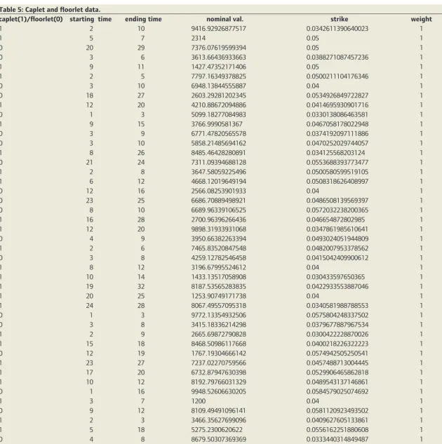
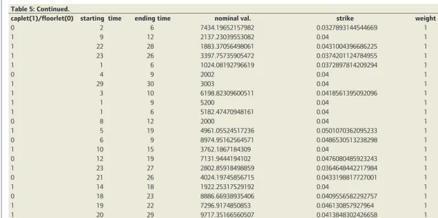
Table 5: Caplet and fl oorlet data.
caplet(1)/fl oorlet(0) starting time ending time nominal val. strike weight price
1 2 10 9416.92926877517 0.0342611390640023 1 1200
1 5 7 2314 0.05 1 100
0 20 29 7376.07619599394 0.05 1 200
0 3 6 3613.66436933663 0.0388271087457236 1 205
1 9 11 1427.47352171406 0.05 1 60
1 2 5 7797.16349378825 0.0500211104176346 1 450
0 3 10 6948.13844555887 0.04 1 310
0 18 27 2603.29281202345 0.0534926849722827 1 90
1 12 20 4210.88672094886 0.0414695930901716 1 290
0 1 3 5099.18277084983 0.0330138086463581 1 210
1 9 15 3766.9990581367 0.0467058178022948 1 230
0 3 9 6771.47820565578 0.0374192097111886 1 325
0 3 10 5858.21485694162 0.0470252029744057 1 350
1 8 26 8485.46428280891 0.034125568203124 1 1700
0 21 24 7311.09394688128 0.0553688393773477 1 250
1 2 8 3647.58059225496 0.0500580599519105 1 230
1 6 12 4668.12019649194 0.0508318626408997 1 270
0 12 16 2566.08253901933 0.04 1 95
0 23 25 6686.70889498921 0.0486508139569397 1 170
0 8 10 6689.96339106525 0.0572032238200365 1 360
1 16 28 2700.96396266436 0.046654872802985 1 175
1 12 20 9898.31933931068 0.0347861985610641 1 820
0 4 9 3950.66382263394 0.0493024051944809 1 280
1 2 6 7465.83520847548 0.0482007953378562 1 500
0 3 8 4259.12782546458 0.0415042409900612 1 256
1 8 12 3196.67995524612 0.04 1 210
1 10 14 1433.13517058908 0.030433597650365 1 96
1 19 32 8187.53565283835 0.0422933553887046 1 600
1 20 25 1253.90749171738 0.04 1 52
1 24 28 8067.49557095318 0.0340581988788553 1 260
0 1 3 9772.13354932506 0.0575804248337502 1 609
0 3 8 3415.18336214298 0.0379677887967534 1 180
1 2 9 2665.69872790828 0.0300422228870026 1 315
1 15 18 8468.50986117668 0.0400218226322223 1 350
0 12 19 1767.19304666142 0.0574942505250541 1 90
1 23 27 7237.02270759566 0.0457488713004445 1 210
1 17 20 6732.87947630398 0.0529906465862818 1 212
1 10 12 8192.79766031329 0.0489543137146861 1 326
0 1 16 9948.52606630205 0.0584579025074692 1 525
1 3 7 1200 0.04 1 92
0 9 12 8109.49491096141 0.0581120923493502 1 500
1 2 3 3466.35627699096 0.0409627605133861 1 130
1 5 18 5275.2300620622 0.0556162251880608 1 380
0 4 8 8679.50307369369 0.0333440314849487 1 410
1 18 22 6007.33779722487 0.0432106019483251 1 220
1 2 6 791.972365347071 0.04 1 56
1 28 29 8255.73661136544 0.0455450500767311 1 90
1 14 17 5539.87536936097 0.0509304193428627 1 201
0 10 12 1007.22151059842 0.0590681356060862 1 45
34-44_Kienitz_Part_II_TP_March_241 41
42
Wilmott
magazine
Figure 2: Calibration error for Hull–White model to market prices from Table 5. The
x-axes are the used options and the
y-axes are the
option prices, resp. the error in %
{ (...)
SumDiscountFactor += exp(-intR); }
(...)
itsDiscountFactor = SumDiscountFactor / itsNSIM;.
The variable names should explain what they stand for. This completes the discussion of implementation. We will now proceed to some experi-ments with our model.
4 Numerical Example and Extensions
4.1 Numerical Example
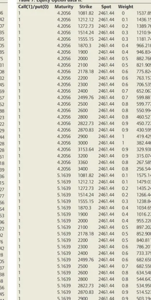
Finally, we show the result of a calibration of the Heston–Hull–White model to market prices. The market prices are summarized in section 5. To this end
we calibrate the Hull–White model to an initial yield curve, Table 4, as well as to caps and floors, Table 5. The other parameters are then calibrated using the previously calibrated Hull-White parameters. We show the calibration results and compare the results to a calibration of a Heston model. We use tables 6 and 7. First, we consider the calibration of the Hull–White model to caplet and floorlet prices as well as the given yield curve. We show the cali-bration results in Figure 2.
Second, we consider the calibration of the Heston–Hull–White model and a Heston model to the same call and put prices. Figure 3 shows the calibration error of both models and also the prices from both models with respect to the market prices are given.
[image:9.866.95.732.97.414.2]Summarizing we remark that for long dated options, especially if they are
out–of–the–money, the Heston–Hull–White model shows superior results to the Heston model.Table 5: Continued.
caplet(1)/fl oorlet(0) starting time ending time nominal val. strike weight price
0 2 6 7434.19652157982 0.0327893144544669 1 350
1 9 12 2137.23039553082 0.04 1 110
1 22 28 1883.37056498061 0.0431004396686225 1 65
1 23 26 3397.75735905472 0.0374201124784955 1 100
1 1 6 1024.08192796619 0.0372897814209294 1 90
0 4 9 2002 0.04 1 106
1 29 30 3003 0.04 1 55
1 3 10 6198.82309600511 0.0418561395092096 1 535
1 1 9 5200 0.04 1 540
1 1 6 5182.47470948161 0.04 1 420
0 8 12 2000 0.04 1 85
1 5 19 4961.05524517236 0.0501070362095233 1 480
0 6 9 8974.95162564571 0.0486530513238298 1 520
1 10 15 3762.1867184309 0.04 1 220
0 12 19 7131.9444194102 0.0476080485923243 1 260
1 23 27 2802.85918498859 0.0364648442217984 1 100
0 21 26 4024.19745856715 0.0433198817727001 1 95
1 14 18 1922.25317529192 0.04 1 100
0 18 23 8886.66938935406 0.0409556582292757 1 225
1 19 22 7296.9174850853 0.046130857927964 1 240
1 20 29 9717.35166560507 0.0413848302426658 1 450
34-44_Kienitz_Part_II_TP_March_242 42
Wilmott
magazine
43
[image:10.866.78.647.92.742.2]^
Table 6: Equity option data I.
Call(1)/put(0) Maturity Strike Spot Weight Price
1 1.1944 1081.82 2461.44 0.1 1422.3792940646
1 1.1944 1212.12 2461.44 0.2 1300.25370868542
1 1.1944 1272.73 2461.44 0.3 1243.99130024807
1 1.1944 1514.24 2461.44 0.4 1024.24909532335
1 1.1944 1555.15 2461.44 0.5 987.873233682635
1 1.1944 1870.3 2461.44 0.6 718.504165558505
1 1.1944 1900 2461.44 0.7 694.553484851185
1 1.1944 2000 2461.44 0.7 616.07786707975
1 1.1944 2100 2461.44 0.7 541.352430949431
1 1.1944 2178.18 2461.44 0.8 485.476234822808
1 1.1944 2200 2461.44 0.8 470.355265362432
1 1.1944 2300 2461.44 0.8 403.619865578245
1 1.1944 2400 2461.44 0.9 341.329392723369
1 1.1944 2499.76 2461.44 0.9 284.662130191257
1 1.1944 2500 2461.44 1 284.551671409552
1 1.1944 2600 2461.44 1 234.394879670288
1 1.1944 2800 2461.44 0.9 150.466033702423
1 1.1944 2822.73 2461.44 0.9 142.703361496322
1 1.1944 2870.83 2461.44 0.8 126.795377812929
1 1.1944 2900 2461.44 0.8 117.874621567444
1 1.1944 3000 2461.44 0.7 90.6649710320428
1 1.1944 3153.64 2461.44 0.7 61.1561444384128
1 1.1944 3200 2461.44 0.6 54.0033253306561
1 1.1944 3360 2461.44 0.5 34.3977917525318
1 1.1944 3400 2461.44 0.4 30.5318701182539
1 2.1916 1081.82 2461.44 0.1 1461.57788048036
1 2.1916 1212.12 2461.44 0.1 1347.09382355315
1 2.1916 1272.73 2461.44 0.2 1294.64533887627
1 2.1916 1514.24 2461.44 0.2 1091.46437642577
1 2.1916 1555.15 2461.44 0.3 1058.03626462066
1 2.1916 1870.3 2461.44 0.4 811.975310510654
1 2.1916 1900 2461.44 0.5 789.914122496853
1 2.1916 2000 2461.44 0.6 717.153979232596
1 2.1916 2100 2461.44 0.7 648.130294235522
1 2.1916 2178.18 2461.44 0.7 596.11622818202
1 2.1916 2200 2461.44 0.7 581.90113391976
1 2.1916 2300 2461.44 0.8 518.724821472442
1 2.1916 2400 2461.44 0.8 458.76104598328
1 2.1916 2499.76 2461.44 0.9 402.277440098405
1 2.1916 2500 2461.44 0.9 402.168322491237
1 2.1916 2600 2461.44 1 352.800681959238
1 2.1916 2800 2461.44 1 265.29815191738
1 2.1916 2822.73 2461.44 0.9 256.258466145666
1 2.1916 2870.83 2461.44 0.9 237.788657548345
1 2.1916 2900 2461.44 0.8 227.112201880144
1 2.1916 3000 2461.44 0.8 193.737434726345
1 2.1916 3153.64 2461.44 0.7 149.226004850452
1 2.1916 3200 2461.44 0.6 137.377308320527
1 2.1916 3360 2461.44 0.5 101.043834423851
[image:10.866.387.700.110.730.2]1 2.1916 3400 2461.44 0.4 93.1568497899167
Table 7: Equity Option data II.
Call(1)/put(0) Maturity Strike Spot Weight Price
1 4.2056 1081.82 2461.44 0 1537.89780938587
1 4.2056 1212.12 2461.44 0.1 1436.15374265053
1 4.2056 1272.73 2461.44 0.2 1389.76521576543
1 4.2056 1514.24 2461.44 0.3 1210.94634749796
1 4.2056 1555.15 2461.44 0.3 1181.7432801964
1 4.2056 1870.3 2461.44 0.4 966.218070719351
1 4.2056 1900 2461.44 0.4 946.834481174701
1 4.2056 2000 2461.44 0.5 882.766031799261
1 4.2056 2100 2461.44 0.5 821.909315912906
1 4.2056 2178.18 2461.44 0.6 775.824412354643
1 4.2056 2200 2461.44 0.6 763.157788414055
1 4.2056 2300 2461.44 0.6 706.535835262685
1 4.2056 2400 2461.44 0.7 652.067710023196
1 4.2056 2499.76 2461.44 0.7 599.881006918677
1 4.2056 2500 2461.44 0.8 599.777598336201
1 4.2056 2600 2461.44 0.8 550.994727629446
1 4.2056 2800 2461.44 0.8 460.521491020263
1 4.2056 2822.73 2461.44 0.9 450.727847025402
1 4.2056 2870.83 2461.44 0.9 430.599084642388
1 4.2056 2900 2461.44 1 419.429846883366
1 4.2056 3000 2461.44 1 382.44604273531
1 4.2056 3153.64 2461.44 0.9 329.938079701859
1 4.2056 3200 2461.44 0.9 315.074022307316
1 4.2056 3360 2461.44 0.8 267.585053775738
1 4.2056 3400 2461.44 0.8 256.544421518989
1 5.1639 1081.82 2461.44 0.1 1575.14545916331
1 5.1639 1212.12 2461.44 0.1 1479.03073519054
1 5.1639 1272.73 2461.44 0.2 1435.24541401566
1 5.1639 1514.24 2461.44 0.2 1266.44917918489
1 5.1639 1555.15 2461.44 0.3 1238.84605922055
1 5.1639 1870.3 2461.44 0.4 1034.69682580327
1 5.1639 1900 2461.44 0.4 1016.27541291196
1 5.1639 2000 2461.44 0.4 955.220133255394
1 5.1639 2100 2461.44 0.5 897.202261867494
1 5.1639 2178.18 2461.44 0.5 852.900221803726
1 5.1639 2200 2461.44 0.5 840.811112260794
1 5.1639 2300 2461.44 0.6 786.201108526362
1 5.1639 2400 2461.44 0.6 733.379712207143
1 5.1639 2499.76 2461.44 0.6 682.650495178919
1 5.1639 2500 2461.44 0.7 682.550238143673
1 5.1639 2600 2461.44 0.8 634.54817806271
1 5.1639 2800 2461.44 0.8 544.647852148374
1 5.1639 2822.73 2461.44 0.8 534.950590253353
1 5.1639 2870.83 2461.44 0.9 514.523135676212
1 5.1639 2900 2461.44 0.9 503.194830396318
1 5.1639 3000 2461.44 1 465.409173492743
1 5.1639 3153.64 2461.44 1 411.19105063511
1 5.1639 3200 2461.44 0.9 395.583928285715
1 5.1639 3360 2461.44 0.9 345.05333748364
1 5.1639 3400 2461.44 0.8 333.137714853179
34-44_Kienitz_Part_II_TP_March_243 43
44
Wilmott
magazine
4.2 Extensions
We stress the point that the model is easily extendable to a Bates–Hull– White model since it is commonly assumed that the jumps in the Bates model are independent of the volatility and the interest rates. Therefore, the implementation corresponds to a multiplication of the characteristic function.
Furthermore, it is possible to compute greeks very efficiently. Table 3 summarizes the possible extensions we have implemented. The results have been produced using the following parameters T = 10, K = 100, S(0) = 95, r = 4.09% and ˜v = 0.02, v(0) = 0.02, κ = 0.2, r = −0.6, v = 0.5 for the Heston dynamic as well as s = 0.05, κ = 0.3 for the Hull–White model and finally, for the jump component λ = 0.2 (jump intensity), sJ = 0.05 (jump volatility) and μ J = 0.2 (average jump size).
5 Market Data
This section contains the used market data for the yield curve, caplets, floorlets, and the index options.
Holger Kammeyer is studying toward his Ph.D. in mathematics. He researches geometric L2 invariants. He holds a diploma (with distinction) in mathematics from the University of Goettingen. Before he started his Ph.D. research, he worked as a teaching assistant, did an internship at Deutsche Postbank with the Quantiative Analysis group, and completed a one year graduate study at UC Berkeley.
Joerg Kienitz is the head of Quantitative Analysis at Deutsche Postbank AG. He is primarily involved in the development and implementation of models for pricing structured products,
derivatives, and asset allocation. He authored a number of quantitative finance papers and his book “Monte Carlo Frameworks” was published with Wiley in 2009. A new Wiley book,
“Financial Modelling – Theory, Implementatin and Practice with Matlab Source Code” will
REFERENCES
J. Andersen. 2006. Efficient Simulation of the Heston Stochastic Volatility Model. Preprint. M. Attari. 2004. Option pricing using fourier transforms: A numerically efficient simplifica-tion. Working paper, Charles River Associates.
S. Bochkanov. 2010. Alglib financial library. www.alglib.net.
D. Brigo and F. Mercurio. 2006. Interest Rate Models - Theory and Practice, 2nd ed.
Springer, Berlin, Heidelberg, New York.
P. Carr and D. Madan. 1999. Option Valuation using the Fast Fourier Transform. Journal of Computational Finance, (4): 61–73.
J.H. Chan and M. Joshi. 2010. Fast and Accurate Long Stepping Simulation of the Heston Stochastic Volatility Model. Preprint, ssrn.com.
D. Duffy and J. Kienitz. 2009. Monte Carlo Frameworks - Building Customisable and High-performance C++ Applications. John Wiley & Sons, Chichester.
F. Fang and K. Osterlee. 2008. A Novel Pricing Method for European Option based on Fourier-Cosine Series Expansions. Munich Personal RePEc ARchive, 9319.
P. Glasserman and K.-K. Kim. 2008. Gamma Expansion of the Heston Stochastic Volatility Model. Preprint, ssrn.com.
GSL. 2010. Gnu scientific library. www.gnu.org/software/gsl.
A. Lewis. 2000. Option Valuation under Stochastic Volatility. Financepress.
Fang F. Bervoets G. Oosterlee C.W. Lord, R. 2008. A fast and accurate fft-based method for pricing early-exercise options under Lévy processes. SIAM J. Sci Comput.
R. Lord and C. Kahl. 2006. Optimal Fourier inversion in semi-analytical option pricing. Preprint.
[image:11.866.106.668.125.226.2]M. Staunton. 2007. Monte Carlo for Heston. Wilmott magazine May, 70–71. Pelsser A. van Haastrecht, A. 2008. Efficient, almost exact simulation of the Heston stochastic volatility model. Preprint, ssrn.com.
Figure 3: Calibration error of the Heston–Hull–White and the Heston model (left) and the model and market prices (right). The
x-axes are the used
options and the
y-axes is the error in %, resp. the option price. The market data is given by Tables 6 and 7.
be published in spring 2012. He is member of the editorial board of the International Review of Applied Financial Issues and Economics. He holds a Ph.D. in stochastic analysis and probability theory.
W
34-44_Kienitz_Part_II_TP_March_244 44
Financial Risk
Forecasting
The Theory and Practice of
Forecasting Market Risk with
Implementation in R and Matlab
Jón Daníelsson
Financial Risk Forecasting is a complete introduction
to practical quantitative risk management, with a focus on market risk. Derived from the author’s teaching notes and years spent training practitioners in risk management techniques, it brings together the three key disciplines of finance, statistics and modeling (programming), to provide a thorough grounding in risk management techniques.
Written by renowned risk expert Jón Daníelsson, the book begins with an introduction to financial markets and market prices, volatility clusters, fat tails and nonlinear dependence. It then goes on to present volatility forecasting with both univatiate and multivatiate methods, discussing the various methods used by industry, with a special focus on the GARCH family of models.
978-0-470-66943-3 • Hardback • 296 pages March 2011 • £45.00 / €54.00 £27.00 / €32.40
Financial Risk
Management
Models, History, and Institutions
Allan M. Malz
Financial risk has become a focus of financial and nonfinancial firms, individuals, and policy makers. But the study of risk remains a relatively new discipline in finance and continues to be refined. The financial market crisis that began in 2007 has highlighted the challenges of managing financial risk.
Now, in Financial Risk Management, author Allan Malz addresses the essential issues surrounding this discipline, sharing his extensive career experiences as a risk researcher, risk manager, and central banker.
The book includes standard risk measurement models as
well as alternative models that address options, structured credit risks, and the real-world complexities of risk modeling, and provides the institutional and historical background on financial innovation, liquidity, leverage, and financial crises that is crucial to practitioners and students of finance for understanding the world today.
978-0-470-48180-6 • Hardback • 722 pages November 2011 • £65.00 / €76.00 £39.00 / €45.60
An Introduction
to Banking
Liquidity Risk and
Asset-Liability Management
Moorad Choudhry
“A great write-up on the art of banking. Essential reading for anyone working in finance.”
Dan Cunningham, Senior Euro Cash & OBS Dealer, KBC Bank NV, London
“Focused and succinct review of the key issues in bank risk management.”
Graeme Wolvaardt, Head of Market Risk Control, Europe Arab Bank plc, London
The importance of banks to the world’s economic
system cannot be overstated. The foundation of consistently successful banking practice remains efficient asset-liability management and liquidity risk management. This book introduces the key concepts of banking, concentrating on the application of robust risk management principles from a practitioner viewpoint, and how to incorporate these principles into bank strategy.
Written in the author’s trademark accessible style, this book is a succinct and focused analysis of the core principles of good banking practice.
978-0-470-68725-3 • Paperback • 382 pages March 2011 • £34.99 / €42.00 £20.99 / €25.20
Winning at Risk
Strategies to Go Beyond Basel
Annetta Cortez
Navigating the waters of risk and capital management in today’s environment can be intensely challenging. If you are a manager or executive with risk management responsibilities and have not been formally trained as a risk management professional, beware. Risk
management doesn’t lend itself to “do-it-yourself” approaches nor can the essentials be picked up through an instructional video on the ride from the airport to your next meeting.
Designed to help busy executives sort through the complexities of risk management toward developing a holistic, multi-disciplinary, science-based risk and capital management strategy, Winning at Risk: Strategies to Go
Beyond Basel presents a practical perspective to understanding what is important, where to place
focus, and how to use the best of risk and capital capabilities to your business’ advantage. 978-0-470-92466-2 • Hardback • 254 pages • June 2011 • £42.50 / €48.00 £25.50 / €28.80
Book Club
Share our passion for great writing – with Wiley‘s list of titles for independent thinkers ...
SAVE
40%
When you subscribe to Wilmott magazine you will automatically become a member of the Wilmott Book Club and you’ll be eligible for 40 percent discount on specially selected books in each issue. The titles will range from finance to narrative non-fiction. For further information, call our Customer Services Department