Climate-mediated changes to mixed-layer properties in the Southern Ocean: assessing the phytoplankton response

www.biogeosciences.net/5/847/2008/

© Author(s) 2008. This work is distributed under the Creative Commons Attribution 3.0 License.

Biogeosciences

Climate-mediated changes to mixed-layer properties in the Southern

Ocean: assessing the phytoplankton response

P. W. Boyd1, S. C. Doney2, R. Strzepek1,3, J. Dusenberry2, K. Lindsay4, and I. Fung5

1_{NIWA Centre for Chemical and Physical Oceanography, Dept. of Chemistry, University of Otago, Dunedin, New Zealand} 2_{Marine Chemistry and Geochemistry Department, Woods Hole Oceanographic Institution, Woods Hole, MA 02543, USA} 3_{Department of Chemistry, University of Otago, Dunedin, New Zealand}

4_{Climate and Global Dynamics, National Center for Atmospheric Research Boulder, CO 80307, USA}

5_{Department of Earth & Planetary Science, Berkeley Institute of the Environment, Berkeley, CA 94720-1250, USA} Received: 30 October 2007 – Published in Biogeosciences Discuss.: 23 November 2007

Revised: 6 May 2008 – Accepted: 6 May 2008 – Published: 19 May 2008

Abstract. Concurrent changes in ocean chemical and phys-ical properties influence phytoplankton dynamics via alter-ations in carbonate chemistry, nutrient and trace metal inven-tories and upper ocean light environment. Using a fully cou-pled, global carbon-climate model (Climate System Model 1.4-carbon), we quantify anthropogenic climate change rela-tive to the background natural interannual variability for the Southern Ocean over the period 2000 and 2100. Model re-sults are interpreted using our understanding of the environ-mental control of phytoplankton growth rates – leading to two major findings. Firstly, comparison with results from phytoplankton perturbation experiments, in which environ-mental properties have been altered for key species (e.g., bloom formers), indicates that the predicted rates of change in oceanic properties over the next few decades are too sub-tle to be represented experimentally at present. Secondly, the rate of secular climate change will not exceed background natural variability, on seasonal to interannual time-scales, for at least several decades – which may not provide the pre-vailing conditions of change, i.e. constancy, needed for phy-toplankton adaptation. Taken together, the relatively subtle environmental changes, due to climate change, may result in adaptation by resident phytoplankton, but not for several decades due to the confounding effects of climate variabil-ity. This presents major challenges for the detection and at-tribution of climate change effects on Southern Ocean phy-toplankton. We advocate the development of multi-faceted

Correspondence to: P. W. Boyd ([email protected])

tests/metrics that will reflect the relative plasticity of different phytoplankton functional groups and/or species to respond to changing ocean conditions.

1 Introduction

Climate change impacts ocean biota in many ways, and sub-sequently biological feedbacks may amplify or dampen any initial climate change signal (Denman et al., 1996; Boyd and Doney, 2003; Fung et al., 2005). These feedbacks arise from both changes in bulk properties (primary production) and in floristics (e.g. diatoms versus coccolithophores) (Boyd and Doney, 2002). Coupled Ocean-Atmosphere Model (COAM) experiments indicate that ocean physical circulation and chemical properties will shift significantly in the coming decades (Sarmiento et al., 1998; Matear and Hirst, 1999). For the Southern (S.) Ocean, surface waters are projected to be warmer and fresher, with increased vertical stratification, shallower mixed-layer depths, reduced sea-ice, and higher oceanic CO2 concentrations. Recent experiments indicate that S. Ocean westerly winds may increase in strength and shift poleward, increasing upwelling (Russell et al., 2006). Alteration of these upper ocean properties will affect phyto-plankton dynamics and growth rates directly and indirectly through modifications of vertical nutrient supply, mixed-layer depth, and light climate (Bopp et al., 2001).

biological detail, such as algal functional groups (Iglesias-Rodriguez et al., 2002; Le Qu´er´e et al., 2005; Litchman et al., 2006) or foodwebs (Legendre and Rivkin, 2005). Re-cent experimental approaches have conRe-centrated on pertur-bation studies (weeks to months) of phytoplankton responses to light climate, CO2 or nutrient concentrations, in labora-tory cultures (Riebesell et al., 2000), shipboard experiments (Tortell et al., 2002; 2008), mesocosms (DeLille et al., 2005; Riebesell et al., 2007) or 50–200 km2in-situ patches of the ocean (Boyd et al., 2007).

Two steps are required to explore the relationship be-tween climate-change mediated alteration of ocean proper-ties and the consequent phytoplankton response on interme-diary time-scales, i.e. decades – relevant to present experi-mental and observing system design and to policy makers (Dilling et al., 2003). First, models must provide estimates of future ocean environmental changes, and separate the effects of climate change from intrinsic interannual variability. Cur-rently, COAM’s provide one of the few plausible means to do this (Fung et al., 2005; Friedlingstein et al., 2006), and also offer the improved regional predictions needed to predict the rate of climate-mediated change in environmental properties for oceanic provinces.

Second, phytoplankton perturbation experiments must in-clude realistic timescales for the alteration of environmental properties, quantify the potential for physiological plasticity or adaptability of organisms to climate perturbations, and in-vestigate potential synergistic effects due concurrent changes in environmental drivers (e.g. iron and light). Initial exper-iments used large instantaneous perturbations (from 350 to 750µatm CO2, an IPCC climate-change scenario), result-ing in altered calcification rates (Riebesell et al., 2000) or floristic shifts (Tortell et al., 2002). Such striking results rep-resent an upper bound of the effects of climate-change me-diated alterations in environmental forcing on phytoplank-ton processes. However, it is problematic to relate the re-sults from such large, instantaneous perturbations, to the timescales and magnitude of climate change that phytoplank-ton will actually be exposed to. Phytoplankphytoplank-ton can respond to environmental change hours (e.g., algal photoacclimation, Falkowski and LaRoche, 1991), days/weeks (floristic shifts, Riebesell, 1991), to months/years (regime shifts, Boyd and Doney, 2003). This broad range of responses spans the transition from phytoplankton acclimation to adaptation (see Falkowski and LaRoche, 1991).

Here, we compare model estimates of the rates of change in ocean properties due to anthropogenic climate change with results from phytoplankton manipulation experiments, in which these properties have been altered for S. Ocean bloom-forming species (i.e. we recognize the importance of climate effects on higher trophic levels but do not explore this topic here). Moreover, we examine the magnitude and sign of the S. Ocean climate-change and variability signa-tures, and discuss their implications for phytoplankton accli-mation (versus adaptation) to environmental change. These

results will inform us of whether the changes in upper ocean properties, and their impact on the biota, will be detectable over the coming decades, and how to design experiments to adequately represent these changes. If we can design such experiments, our findings will lead to improved attribution of the underlying natural and anthropogenic mechanisms driv-ing such changes in the ocean, providdriv-ing direct tests for the predictions made by numerical models used for future cli-mate projections and policy decisions.

2 Methods and site selection

In this study, we focus on the S. Ocean – a region reported to have a disproportionately large impact on global climate (Sarmiento et al., 1998) and which is particularly sensitive to anthropogenic climate warming (e.g. Sarmiento et al., 2004). These waters are characterized by both high macronutrient concentrations (except for silicic acid in subpolar waters) and low rates of aerosol iron supply (Duce and Tindale, 1991; Fung et al., 2000). Macronutrient concentrations in polar wa-ters are predicted to decrease by only ca. 10% due to climate change (Bopp et al., 2001) and thus the resident phytoplank-ton are unlikely to be subjected to macronutrient limitation.

Phytoplankton in large regions of the S. Ocean are iron-limited, and climate-change driven alterations of ocean physics will likely impact surface iron concentrations. It is not known whether regional dust deposition rates will in-crease or dein-crease due to climate change (Mahowald and Luo, 2003; Moore et al., 2006); likewise predictions of climate-mediated changes in UV irradiance are also incon-clusive (Denman et al., 2007). Thus, the impact of changes in aerosol-iron supply or UV irradiance are not considered further here. In these waters, the biogeography of the key algal functional groups is already well defined, for example there are no nitrogen fixers in the S. Ocean (Westberry and Siegel, 2006), and a southwards decrease in coccolithophore abundance is observed (Cubillos et al., 2007).

2.1 Climate model formulation

requiring surface heat or freshwater flux adjustments. The water cycle is closed through a river runoff scheme.

Biogeochemistry in CSM1.4-carbon is simulated with modified versions of the terrestrial model CASA and the OCMIP-2 oceanic biogeochemistry model (Doney et al., 2004; Najjar et al., 2007). In the fully-coupled carbon-climate model, atmospheric CO2is a prognostic variable and is predicted as the residual after carbon exchanges with the land and ocean. The ocean biogeochemical component in-cludes in simplified form the main processes for the solu-bility carbon pump, organic and inorganic biological carbon pumps, and air-sea CO2flux. The prognostic variables trans-ported in the ocean model are phosphate, total dissolved in-organic, dissolved organic phosphorus, dissolved inorganic carbon, alkalinity, and oxygen.

New/export production is computed prognostically as a function of light, temperature, phosphate and iron concen-trations. The maximum production as a function of tempera-ture is multiplied by nutrient and light limitation terms. The nutrient term is the minimum of Michaelis-Menten limiting terms for PO4and Fe:

FN =min

_PO

4 PO4+κPO4

, Fe

Fe+κFe

(1) whereκPO4is 0.05µmol/L andκFeis 0.03 nmol/L (see later).

The light (irradiance) limitation term:

FI =

I I+κI

, (2)

usesI, the solar short-wave irradiance, and a light limita-tion termκI (20 W/m2). A fully dynamic iron cycle also has been added including atmospheric dust deposition/iron dissolution, biological uptake, vertical particle transport, and scavenging. In the simulations, as a simplification, dust de-posited onto sea-ice is transferred directly to the ocean, with no modification to its properties, such as solubility (see Ed-wards and Sedwick, 2001).

2.2 21st century climate change experiments

A suite of transient experiments (1820–2100) branching off from the stable, pre-industrial control is conducted by speci-fying fossil fuel CO2emissions (Fung et al., 2005). A histori-cal emission trajectory is used for the 19th and 20th centuries and the SRES-A2 “business-as-usual” fossil fuel emission scenario is used for the 21th century. No other greenhouse gases or radiative forcing perturbations are included. Carbon sources associated with anthropogenic land use modification are not included in these experiments. As the other radia-tive forcing nearly cancel in the 19th and 20th centuries, the climate simulation should be broadly comparable to that ob-served in the globally averaged sense. However, over the 19th and 20th centuries, land-use modification accounts for approximately 35% of the cumulative anthropogenic source

of atmospheric CO2. The simulated atmospheric CO2 con-centration in year 2000, therefore, is 20 ppmv too low com-pared to observations (∼367 ppmv), lagging about 12 years behind reality. While the model CO2concentrations cannot be directly matched to calendar years, the overall CO2 tem-poral trends for the 21th century and the year 2100 CO2 con-centration (∼765 ppmv) are comparable to those from other carbon-climate projections (Friedlingstein et al., 2006).

The climate response for a particular variableχ, denoted as1χ (t ), is computed by differencing the transient climate and control simulations at a particular point in timet. The global mean surface air temperature increase 1Tair (2100) is∼1.8 K. Friedlingstein et al. (2006) found that CSM1.4-carbon is at the lower end of reported climate sensitivi-ties, 1Tair/1CO2, relative to several other coupled carbon-climate simulation. In benchmark studies, the transient cli-mate response, i.e. temperature increase at the time of dou-bling of CO2where climate models are forced by a 1% y−1 increase in CO2, is only 1.4 K for the NCAR CSM1.

Therefore, we have also conducted two additional exper-iments for the period 2000–2100 where we have artificially increased the climate sensitivity of the CSM1.4-carbon sim-ulation to span the range observed in other COAM’s. In these experiments, the atmospheric radiation calculations see a higher effective CO2concentration than seen by the land or ocean biogeochemistry. Specifically, an atmospheric CO2 perturbation above pre-industrial levels,1CO2, is computed as:

1CO2=COmodel₂ −COpreind₂ (3)

The anthropogenic CO2 perturbation is multiplied by a factor of 2 and 4 for cases A2-x2 and A2-x4, respectively, and then add back in the preindustrial concentration to find the CO2concentration fed to the model atmospheric radia-tion code:

COradiation₂ =2×1CO2+COpreind₂ ; (4) COradiation₂ =4×1CO2+COpreind₂ (5) Thus, the climate sensitivity to the anthropogenic CO2 per-turbation is effectively enhanced while not directly altering the atmospheric CO2used for air-sea exchange, COmodel₂ . 2.3 Climate change cnalysis

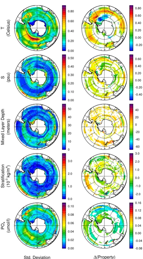
Fig. 1. Annual mean surface water time-series plots (model years 2000–2100) from the control (red) and transient warming simula-tions (IPCC SRES A2 case green; 2x case dark blue; and A2-4x case light blue) averaged over polar waters from the CSM1.4-carbon model. Each panel displays a separate physical or chemical property (temperature, salinity, mixed layer depth, density stratifica-tion, phosphate, dissolved iron,pCO2, incident photosynthetically available radiation, upwelling, and ice fraction). The S. Ocean cli-mate change signals in the transient simulations are approxicli-mately (though not exactly) zonal, and the model Southern Ocean is par-titioned into polar and subpolar waters based on frontal structure, the boundary being set as the simulated 130 Sv streamfunction that approximates well the boundary between the two water masses.

boundary is prescribed from the control simulation stream function and varies from 60–65 deg. S in the Pacific sector to 45–50 deg. S in the Atlantic sector downstream of the Drake Passage. The model ocean stream function evolves with time under climate change because of two factors, an increase in strength and a poleward contraction of the zonal surface wind maximum in the Southern Ocean associated with a shift to-ward more positive phase of the Southern Annular Mode (Russell et al., 2006; Le Qu´er´e et al., 2007; Lovenduski et al., 2007). The effects of the two processes partially counter-act and the lateral shift for the 130 Sv streamline is minimal. In our analysis the subpolar/polar boundary is not allowed to vary through time, which would complicate the comparison with time because it would confound temporal and

geograph-Fig. 2. The same as geograph-Fig. 1 but for subpolar waters.

ical variations. Climate trends are significant only if they differ substantially from the drift of the control simulation, if non-zero, and are larger than the intrinsic interannual vari-ability of the model. For the spatial maps, a Student’s t-test is used to measure the significance of the differences between the two decades relative to the simulated interannual vari-ability. Regions where1χ (2020–2029 minus 2000–2009) is less than the standard deviation ofχfor the decade 2000– 2009 based on a student’st-test are masked out.

2.4 Phytoplankton perturbation experiments

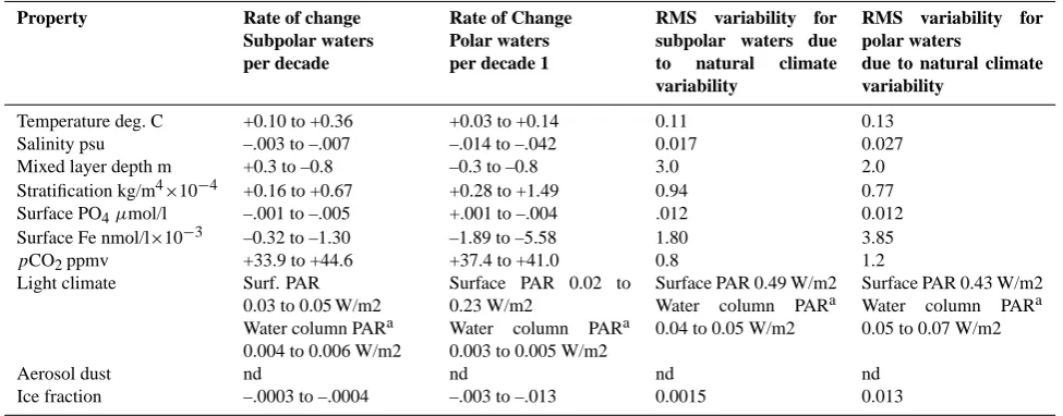
Table 1a. Comparison for S. Ocean sub-polar and polar waters of the relative rate of (a) climate-change mediated alteration of annual-mean ocean properties that influence phytoplankton processes expressed as change per decade compared with; (b) A summary of the range of conditions for each ocean property under which manipulation experiments have been conducted on either key polar bloom-forming species, or natural polar assemblages. The climate change rates in a) are estimated from a suite of fully coupled CSM 1.4-Carbon simulations by spatially averaging over the subpolar or polar domains (boundary defined by the 130 Sv stream function contour) and averaging over the period 2000 and 2100. The model ranges correspond with the simulations with varying model climate sensitivities to atmospheric CO2 perturbations. The model estimated rms variability in annual-mean, spatial averaged ocean properties due to natural climate variability is included for reference. nd denotes uncertainty over sign of change (Mahowald et al., 2005). Due to the paucity of data on the effects of environmental manipulations on sub-polar phytoplankton this summary focuses only on polar waters. However, see studies by Riebesell et al. (2007) and Hutchins et al. (2001).

Property Rate of change Subpolar waters per decade

Rate of Change Polar waters per decade 1

RMS variability for subpolar waters due to natural climate variability

RMS variability for polar waters

due to natural climate variability

Temperature deg. C +0.10 to +0.36 +0.03 to +0.14 0.11 0.13

Salinity psu –.003 to –.007 –.014 to –.042 0.017 0.027

Mixed layer depth m +0.3 to –0.8 –0.3 to –0.8 3.0 2.0

Stratification kg/m4×10−4 +0.16 to +0.67 +0.28 to +1.49 0.94 0.77

Surface PO₄µmol/l –.001 to –.005 +.001 to –.004 .012 0.012

Surface Fe nmol/l×10−3 –0.32 to –1.30 –1.89 to –5.58 1.80 3.85

pCO₂ppmv +33.9 to +44.6 +37.4 to +41.0 0.8 1.2

Light climate Surf. PAR

0.03 to 0.05 W/m2 Water column PARa 0.004 to 0.006 W/m2

Surface PAR 0.02 to 0.23 W/m2

Water column PARa 0.003 to 0.005 W/m2

Surface PAR 0.49 W/m2 Water column PARa 0.04 to 0.05 W/m2

Surface PAR 0.43 W/m2 Water column PARa 0.05 to 0.07 W/m2

Aerosol dust nd nd nd nd

Ice fraction –.0003 to –.0004 –.003 to –.013 0.0015 0.013

a_{surface mixed-layer light climate was derived using mixed layer depth and chlorophyll concentration (as a proxy of light attenuance) as}

detailed in Boyd et al. (2007).

1 W/m2∼0.4 mol quanta m−2d−1from Cloern et al. (1995).

3 Results

3.1 Model simulations

The CSM1.4-carbon results are broadly similar to other COAM simulations that exhibit surface warming of Southern Ocean waters in response to anthropogenic climate change. While the anthropogenic warming signal is quite clear in the CSM1.4-carbon A2 case by the end of the 21st century, the warming trend earlier in the century is less apparent because of natural variability, particularly over shorter time-spans of a couple of decades relevant to the establishment of ocean observing systems. In the low climate sensitivity A2 case, the decadal mean sea surface temperature (SST) in the sub-polar region increases by +0.10 K/decade for a 20-year pe-riod (model years 2020–2029 minus 2000–2009) (Figs. 1– 3; Table 1a). For comparison the root mean squared (rms) variability of the subpolar mean SST on interannual scales is 0.11 K. Given a sampling duration of two to three decades, therefore, the anthropogenic SST warming trend is thus de-tectable, though somewhat marginally, above the natural in-terannual variability for the subpolar region. The secular warming trend is less pronounced in polar waters closer to

Antarctica in the A2 case, about +0.03 K/decade, and the cli-mate change temperature signal does not clearly exceed nat-ural variability (rms 0.13 K) until roughly model year 2060.

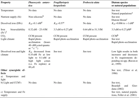
Table 1b. Polar waters

Property Phaeocystis

antarc-tica

Fragillariopsis kerguelenis

Proboscia alata Diatom species or natural populations

Temperature No data No data No data See text

Natural populationsa

Nutrient supply (Si) Non-siliceousb No data No data See text

Diatom bloomc

Dissolved iron (DFe) Km=0.1 nMd Km=0.57e No data Km=0.006 to>1 nMe

Iron bioavailability (Fe’)f

0.32 aM – 25.4 fM 3.5 aM to 0.27 pM 0.64 aM to 51.3 fM 3.5 aM to 0.27 pMg

CO2 CCM present CCM present CCM present CCMh

Light climate Rapid

photo-acclimation (hours 40–400µmol quanta m−1s−1)

Rapid photo-acclimation Rapid photo-acclimation See text

Rapid photo-acclimation

Dissolved iron and light climate

Km decreased from 0.35 nM Fe at low light to 0.1 nM at high light µmax (i.e. Fe replete) at 60µE

See text See text Low light results in both

increases and decreases in Fe requirements de-pending on spp. (Raven et al., 1999)

Other synergistic ef-fects

a) Temperature and light

See text, (Tilzer et al. 1986)

b) Light and CCM’s No data No data No data See text,

Beardall and Gior-dana (2002)

c) Temperature and Fe supply

See text, natural popula-tions, Feller et al. (2001)

a _{Tilzer et al. (1986), Scotia Sea and Bransfield Strait, light-saturated and light-limited photosynthetic rates and their relationship with}

temperature.

b_{altered N:P ratios for P. antarctica relative to diatoms (more efficient N uptake per unit P (Arrigo et al., 1998).}

c_{Nelson et al. (2001) study of silica uptake kinetics along a meridional gradient in silicic acid ranging from<5 in the north to 45µM in the}

South.

d_{Sedwick et al. (2007), effects of iron and light on the growth of natural populations of colonial Phaeocystis antarctica, Ross Sea.} e_{Timmermans et al. (2001),Km(dissolved iron concentration versus growth rate (DFe for 1/2µmax)) for a range of diatoms including}

Chaetoceros brevis (Km0.006) to Actinocyclus (1.14),

f_{Timmermans et al. (2001) used dissolved iron as they could not define Fe bioavailability, and we have used Fe’ as a proxy for bioavailability.} g_{lab culture studies on Southern Ocean polar isolate Eucampia Antarctica (Strzepek, unpublished data).}

h_{CCM’s denote the presence of an inorganic Carbon Concentrating Mechanism. All polar species so far examined (9 diatoms and P.}

antarctica) have all exhibited CCM’s (Tortell et al., 2007).

interannual variability of the real system, we are restricted to comparing long-term secular trends in the model and obser-vations.

With those caveats in mind, the long-term spatial warming patterns in the model are broadly consistent with historical observations (Fig. 3). Like the model, observations exhibit higher surface warming in the Southern Ocean subtropical and subpolar bands than in polar waters, where there has ei-ther been no statistical trend or in some cases weak cooling rather than warming (Smith and Reynolds, 2005; Trenberth

atmospheric surface warming rates for the Southern Ocean region of 0.13+/–0.06 K/decade.

The CSM coupled model warming rates for the last half of 20th century (in model years 2000–2009 minus 1950– 1959 adjusting for the atmospheric CO2delay) are in good agreement with the observed warming. As predicted by other coupled simulations, the model predicted warming rates tend to accelerate in the 21st century, with the simulated warm-ing rates over the next 20 year period of subpolar +0.10 to +0.31 K/decade; polar +0.03 to +0.17) (Figs. 1–3, Table 1).

Both anthropogenic warming and interannual climate vari-ability influence the spatial pattern of regional surface ocean anomalies. The right-hand column of Fig. 3 displays spa-tial maps for difference in simulated surface property be-tween model decade 2020–2029 minus decade 2000–2009 for the A2 case. In the model simulation a zonal band of warmer SSTs occurs in the subtropics and subpolar waters, and a large area of cooling is found in the polar Atlantic sec-tor. The Atlantic regional cooling illustrates an important point that on sub-basin scales interannual climate can slow or even reverse for individual sampling periods the anthro-pogenic warming impacts that are apparent at larger basin and global scales. To focus on the longer term trends in the decadal difference maps in the right-hand column, areas are masked with white if the observed temporal differences are small relative to rms interannual variability.

The magnitude of the interannual variability (rms of an-nual means) in model surface properties is displayed in the left-hand column of Fig. 3. For SST, the regions of maxi-mum interannual variability occur along frontal boundaries, in particular for the example shown in Fig. 3 in Pacific sec-tor along roughly 60 deg. S and in the Atlantic secsec-tor east of South Georgia Island near 30 deg. W. The Southern An-nular Mode (SAM) is a significant contributor to ocean in-terannual variability in the Southern Ocean that reflects the strength of the atmospheric pressure low over the Antarc-tic continent and the high in the subtropics and subpolar re-gion. A positive SAM occurs with an intensification of both the Antarctic low and subtropical high, resulting in field ob-servations and models in stronger westerly winds, increased upwelling, cooler SSTs in polar waters and subpolar central Pacific and warmer SSTs elsewhere in the Southern Ocean (e.g., Lovenduski et al., 2007). The CSM1.4 model decadal SST anomaly patterns with warming of the subpolar zone and neutral or cooling of the polar zone are similar to those observed for a shift to a more positive SAM. The SST pat-terns along with the increased surface winds and upwelling in the simulation are consistent with the argument that anthro-pogenic warming in the S. Ocean will be expressed, in part, through a projection onto an increasing SAM (Le Qu´er´e et al., 2007). The other clear anthropogenic signal is, as would be expected, the increase in surface waterpCO2due to the rise in atmospheric CO2in the transient simulation. North of

∼55◦S, the1pCO2(here transient – control not air – water) tracks the increase in the atmosphere, and absolute values

are 650–800 ppmv by 2100. Poleward of this boundary, the surface water pCO2 increases but not as rapidly as the at-mosphere due to ice cover and the upwelling of older waters from below; average levels are only 500–580 ppmv by 2100. For most of the other physical and biogeochemical fac-tors in the CSM1.4 A2 case, however, the climate change signal is smaller than or comparable to natural variability on the decadal time-scale (2020–2029 minus 2000–2009), mak-ing it difficult to identify anthropogenic signatures. Further, on the sub-basin and basin scale there are regions exhibiting both positive and negative changes over decadal time peri-ods. This is illustrated in the spatial difference maps (decade 2020–2029 minus decade 2000–2009) for case A2 displayed in Fig. 3. For example, the differences maps of mixed layer depth and stratification show no distinct patterns of the cli-mate warming signal evident later in the century – reduced mixed layer depth in polar waters due to freshening, in-creased mixed layer depth in subpolar waters due to stronger winds, and increased vertical stratification in both polar and subpolar waters due to surface freshening and warming, re-spectively (see temporal trends in Figs. 1 and 2).

The large white regions in both maps indicate model points where the decadal changes in mixed layer depth or stratifi-cation are so small that they are not statistically significant relative to the model interannual variability. The simulation also exhibits nearly as many areas of decreasing stratification (green/blue) as increasing stratification (yellow/orange). In-deed, based on the time-series plots averaged over the subpo-lar and posubpo-lar regions, a definitive basin-scale climate warm-ing signal or elevated stratification for the A2 case would not be observable until roughly 2040 (polar) and 2070 (subpo-lar); the threshold for detecting shallower mixed layer depth is also about 2040 for polar waters and is not found by the end of the 21st century in subpolar waters.

The anthropogenic climate signals become more distinct for the in the A2-x2 and A2-x4 cases, with increased climate sensitivity for the following properties: decreasing polar sea surface salinity, increased subpolar and polar stratification, decreased subpolar and polar surface dissolved iron concen-trations, poleward shift and increased strength in polar up-welling, and increased polar surface ocean irradiance due to decreased ice fraction. In higher climate sensitivity cases, the date at which the anthropogenic signal is detectable from the natural background also occurs earlier in time, often by decades.

Fig. 3. Spatial maps of S. Ocean interannual variability and anthro-pogenic climate response from the CSM1.4-carbon transient IPCC SRES A2 simulation. The left column shows the natural interannual variability, expressed as the standard deviation of the annual means from a 10 year segment of the control simulation; the right column shows the climate response expressed as the temporal difference over a 20 year time period, the average of model years 2020-2029 minus the average of model years 2000–2009. Each row displays a separate surface water physical or chemical property (temperature, salinity, mixed layer depth, density stratification, phosphate, dis-solved iron,pCO2, incident photosynthetically available radiation, upwelling, and ice fraction). Regions where the absolute value of the temporal difference is less than one standard error of the differ-ence between the means are masked out.

∂χ

∂t + ∇h·(uχ )− ∇H·(KH∇Hχ )+uZ ∂ ∂zχ

−∂

∂zKZ ∂

∂zχ =RHSbio (6)

where the physical transport is partitioned into horizontal and vertical advection and mixing terms; the biological sur-face uptake and subsursur-face remineralization are grouped into a single biogeochemical right hand side term RHSbio. In-creased stratification and shallower mixed layers tend to de-crease the mixingKZ, while shifts in wind patterns may tend to increase upwellinguZ while decreasing surface resident time-scales.

In CSM1.4, surface nutrient concentrations tend to stay constant or decrease. Phosphate exhibits a small decline from 40–60◦S on average and is constant from 60◦S to the pole. Phosphate concentrations remain large relative toκPO4 and

do not become limiting to organic matter production and ex-port (Eq. 1). There are more notable decreases in surface dis-solved iron concentrations, –5 to –10 pmol/l relative to mean levels of 80–160 pmol/l for 40–60◦S and –20 to –30 pmol/l relative to mean levels of 150–240 pmol/l south of 60◦S. For comparison, the model half saturation constant for al-gal iron limitation for biological organic matter export κFe is 30 pmol/l (i.e. towards the lower end of published values) The trends in surface macro- and micro-nutrients, along with the light/mixed layer and SST in turn impact the downward export flux (Eqs. 1 and 2). Integrated over the entire S. Ocean (including the subtropics), simulated organic matter export remains about the same, though it tends to shift poleward due to the southward migration in the band of deep winter mixing and the expansion of subtropical conditions. In the subpolar region, downward export increases by∼10–15% in October and July while it tends to decrease further south.

Table 2a. Polar waters.

Summary of seasonal ranges for (a) the polar waters of the Ross Sea; and (b) for subpolar waters S of New Zealand (i.e. S of the STF and N of the SAF).

Mixed layer Property Seasonal range Reference

Incident irradiance 6–56 mol quanta m−2d−1 Hiscock et al. (2001)

Mixed layer depth <40 m to>100 m Measures and Vink

Nitrate 34 to<20µmol L−1 Gordon et al. (2000)

Silicic acid 74 to 66µmol L−1 Gordon et al. (2000)

tCO2 2140 to 2260µmol Kg−1 Gordon et al. (2000)

Dissolved iron 0.22 to 0.1 nmol L−1 Measures and Vink (2001)

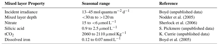
Table 2b. Subpolar waters.

Mixed layer Property Seasonal range Reference

Incident irradiance 13–45 mol quanta m−2d−1 Boyd (unpublished data)

Mixed layer depth <30 m to>120 m Nodder et al. (2005)

Nitrate 15 to<6µmol L−1 Sherlock et al. (2006)

Silicic acid 0.9 to 2.5µmol L−1 S. Pickmere (unpublished data)

tCO2 2060 to 2110µmol Kg−1 K. Currie (unpublished data)

Dissolved iron 0.12 to 0.07 nmol L−1 Boyd et al. (2005)

Broadly similar physical climate response patterns have been found in other 21st century coupled ocean-atmosphere climate simulations, though as mentioned above the CSM1.4-carbon model tends to be at the low end of the range in terms of climate sensitivity to atmospheric CO2 per-turbations. Using a series of empirical diagnostic calcula-tions, Sarmiento et al. (2004) examined the potential ma-rine ecological responses to climate warming using physical data from six different coupled climate model simulations, including a variant of CSM 1. Averaged over the models, climate warming led to a contraction of the highly produc-tive marginal sea ice biome and expansion of the subpolar gyre biome and low productivity, permanently stratified sub-tropical gyre biome in the S. Ocean. Vertical stratification tends to increase, which would be expected to decrease nu-trient supply everywhere but also increase the growth season in some high latitude regions (Sarmiento et al., 2004). They did not investigate the magnitude of upwelling other than in defining the boundaries and shifts in biomes. Sarmiento et al. (2004) suggest that chlorophyll will increase in the open S. Ocean, due primarily to the retreat of and changes at the northern boundary of the marginal sea ice zone; but chloro-phyll may tend to decrease adjacent to the Antarctic conti-nent due primarily to freshening within the marginal sea ice zone. Estimated primary productivity generally will increase mainly as a result of warmer temperatures.

The climate-change driven trends in surface water proper-ties in the Southern Ocean do not occur independently, and

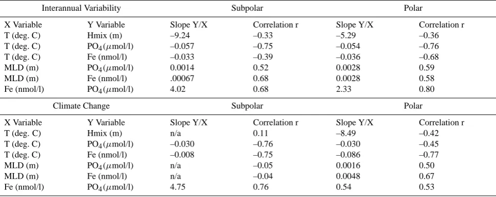
Table 3. A summary of the co-variation of physical and biogeochemical property anomalies due to climate change. Each entry in the table reports the linear regression coefficients (slope and correlation coefficient) for the spatial anomalies from the CCSM1.4-carbon simulation for either interannual variability (monthly values from 100 years of control simulation) or anthropogenic climate change (found from differencing the A2 case decadal average maps 2020–2029 minus 2000–2009; Fig. 3). Separate regressions are computed for the subpolar and polar domains. No slope is reported for regressions where the absolute value of the correlation coefficient is less than 0.2. MLD denotes mixed layer depth.

Interannual Variability Subpolar Polar

X Variable Y Variable Slope Y/X Correlation r Slope Y/X Correlation r

T (deg. C) Hmix (m) –9.24 –0.33 –5.29 –0.36

T (deg. C) PO4(µmol/l) –0.057 –0.75 –0.054 –0.76

T (deg. C) Fe (nmol/l) –0.033 –0.39 –0.036 –0.68

MLD (m) PO4(µmol/l) 0.0014 0.52 0.0028 0.59

MLD (m) Fe (nmol/l) .00067 0.68 0.0028 0.58

Fe (nmol/l) PO4(µmol/l) 4.02 0.68 2.33 0.80

Climate Change Subpolar Polar

X Variable Y Variable Slope Y/X Correlation r Slope Y/X Correlation r

T (deg. C) Hmix (m) n/a 0.11 –8.49 –0.42

T (deg. C) PO4(µmol/l) –0.030 –0.76 –0.030 –0.45

T (deg. C) Fe (nmol/l) –0.008 –0.75 –0.086 –0.77

MLD (m) PO4(µmol/l) n/a –0.05 0.0016 0.50

MLD (m) Fe (nmol/l) n/a –0.04 0.0048 0.67

Fe (nmol/l) PO4(µmol/l) 4.75 0.76 0.54 0.53

analysis suggested that interannual variability is only a weak analogue for climate change with respect to synergistic and non-linear interactions across multiply variables.

3.2 Polar phytoplankton responses to environmental per-turbations

Physiological responses of both laboratory-cultured species and natural assemblages to altered environmental conditions are summarized (Table 1b). The range of conditions used in experiments is readily compared to predicted changes in these properties due to climate change (Table 1). Tilzer et al. (1986) investigated temperature effects on photosyn-thetic performance in cells from the Scotia Sea and Brans-field Strait. They expressed temperature effects usingQ10 – a commonly used temperature coefficient which provides a measure of the rate of change of algal physiology due to a 10◦C increase in temperature. Light-saturated photosyn-thesis (Pbmax) increased significantly with increasing tem-peratures from –1–.5◦_{C to 8}◦_{C, c.f. Table 1a). The} great-est enhancement of Pbmax occurred between –1.5◦C and 2◦C (Q10>4), but decreased at temperatures of>2 to 5◦C, (Q10 of 2.6), and at >5◦C was negligible. This response illustrates the high sensitivity of polar organisms to temper-ature (Clarke, 2003). Studies on coastal phytoplankton in-dicate that a 1◦C–2◦C warming around the Antarctic Penin-sula might not alter photosynthetic rates, but could channel more photosynthetically fixed carbon into DOC (Moran et

al., 2006). Also in these waters, Moline et al. (2004) reported floristic shifts from diatoms to chrysophytes, between 1991 and 1996, associated with warmer temperatures and a conse-quent reduction in salinity. Thus, warming can both directly and indirectly impact phytoplankton processes, and probably influences polar (e.g. ice melt,Q10)waters to a greater extent than sub-polar regions.

Manipulation of either light climate or CO2concentrations appear to have relatively little effect on polar species. Cul-tured polar phytoplankton can rapidly acclimate to a two- to three-fold range of irradiances on a timescale of hours to days (R. Strzepek, unpublished data) Such photoacclimation has been widely reported for non-polar species (Falkowski and LaRoche, 1991). The maximum growth rate of Phaeocys-tis antarctica occurs at∼60µmol quanta m−2s−1(Table 1b), and declines rapidly at lower irradiances, whereas at higher than saturating irradiances their growth rate decreases but at a much slower rate (R. Strzepek, unpublished data). This trend is also observed for cultured polar diatoms (R. Strzepek, un-published data). Predictions in Table 1a indicate that in-creased mean irradiances, due to a shoaling of the mixed layer, will occur with climate change. However, this increase is probably too subtle to result in a detectable alteration of phytoplankton growth rates.

Some phytoplankton species have Carbon Concentrating Mechanisms (CCM’s) which permit them to compensate, via active intracellular accumulation, for the large difference (ranging from 5- to 20-fold) between the CO2 concentra-tion in the surrounding waters with that within their cel-lular machinery (Kaplan et al., 1991). Beardall and Gior-dana (2002), reviewed phytoplankton CCM’s and suggest that rising ocean CO2concentrations may impact the perfor-mance of groups with (diatoms) and without (chrysophytes) CCM’s. Rost et al. (2003) examined representative bloom-formers (diatom, coccolithophorid, and Phaeocystis) accli-mated to 36–1800 ppmv CO2. They reported major differ-ences in the ability of each species to both regulate carbon acquisition and in the efficiency of carbon acquisition. In the most comprehensive study of CCM’s in S. Ocean biota to date, Tortell et al. (2008) present evidence of the presence of inorganic CCM’s (i.e. i.e. cells transporting HCO−₃ and utilizing carbonic anhydrase to catalyze HCO3 dehydration to CO2)for each of ten polar species, including Phaeocys-tis antarctica, and Fragilariopsis kerguelensis, they investi-gated. This widespread presence of CCM’s is evident for mixed assemblages in the subpolar Bering Sea (Martin et al., 2006) and NE Pacific (Tortell et al., 2006). Thus, it is dif-ficult to predict whether any particular species would have a selective advantage to utilize CO2 at the predicted higher concentrations (Table 1a).

In contrast to light climate and CO2 concentrations, changes in dissolved iron concentrations had a pronounced effect on the growth rate (i.e.Km, see Table 1b) of different polar species in culture, regardless of whether iron supply was expressed as dissolved iron or bioavailable/free Fe (Ta-ble 1b). Although there are difficulties in defining what con-stitutes bioavailable iron, that confound the comparison of model parameterizations with observational data, the range of dissolved iron concentrations (that set half the maximum algal growth rate) in Table 1b is considerably greater than predicted changes in dissolved iron concentrations due to climate change (Table 1a). Polar diatoms generally

exhib-ited higher values ofKmthan for Phaeocystis antarctica (Ta-ble 1b), indicative of a greater sensitivity to future decreases in dissolved iron predicted by the model (Table 1a).

There are few studies of the synergistic effects due to si-multaneous limitation (or its alleviation) of algal growth by multiple environmental factors. Takeda (1998) reported in-creased silicification rates at low, relative to high, dissolved iron concentrations in two cultured polar diatoms: silicifi-cation will be altered by both iron and silicic acid supply, two properties that will be influenced by climate change (Ta-ble 1a). Beardall and Giordano (2002) concluded that factors which may impact algal CCM’s include CO2concentrations, temperature and also UV-B radiation. In SW Atlantic polar waters, Feller et al. (2001) reported that both SST and low dissolved iron concentrations limited growth rates of resident phytoplankton. These studies all point to the complex inter-actions between environmental properties that will be altered concurrently by climate change (Table 1a).

Other synergistic effects include iron and irradiance, and studies of iron/light interactions have reported up to threefold reductions inKmfor colonial Phaeocystis antarctica follow-ing transfer from low to high light conditions (Sedwick et al., 2007; Table 1b). Strzepek (Table 1b) observed that, for three cultured Thalassiosira species and Phaeocystis antarc-tica (non-colonial), the greatest effect of iron-limitation is observed at higher growth irradiances, i.e.µ/µmax is lower at higher light levels (whereµdenotes Fe-limited andµmax represents Fe-replete growth rates). His findings differ from reports that low irradiance exacerbate algal iron require-ments (Timmermans et al., 2001; Maldonado et al., 1999); this disparity may result from the use of different cultured species, or different methodologies (acclimated versus non-acclimated; i.e. Timmermans et al.; cultures). Raven et al. (1999) suggest that low light results in both increases and decreases in algal iron requirements depending on species.

4 Discussion

4.1 Climate-change mediated alteration of ocean properties – response of the phytoplankton

will be of limited value for predicting the algal response to climate change. Such perturbations provide no information on the potential for physiological plasticity for different phy-toplankton groups or species. Such information is needed to gauge whether different groups will adapt to the more grad-ual trends in environmental properties that will occur due to climate change. Representation of these gradual environ-mental changes, for example, would require slow increases in CO2of 3–4 ppmv yr−1for six months to several years. Such an experiment, albeit with a small change in CO2, might permit extrapolation of the observed response of different species to perturbation, and would refine the approaches used previously (i.e. large instantaneous perturbations, Riebesell et al., 2000). But artifacts due to bottle or mesocosm con-tainment (see Beninca et al., 2008) will likely confound any biological response to the climate change signal. Thus, we must explore alternative means to capture, in some way, the effects of relatively slow rates of climate-mediated change on ocean properties.

Although the predicted rate of change in each ocean prop-erty is too subtle to be represented experimentally, it is pos-sible that the potential multiplicative impact of synergistic effects (i.e. simultaneous limitation of algal growth by sev-eral factors) could be reproduced experimentally. Here, we consider iron and light. The model simulations predict lower dissolved iron concentrations and slightly higher underwa-ter light levels (Table 1a), which may result, for some algal species (Raven et al., 1999), in greater simultaneous limita-tion of phytoplankton growth rate by iron and light (i.e. the greatest displacement of growth rates from their maximum, Phaeocystis antarctica, see results). However, any amplifica-tion of the biological signal via a greater phytoplankton phys-iological response to multiple factors (and their alteration by climate-change) may be countered by increased uncertainty, due to increased complexity, in predicting how phytoplank-ton dynamics will change when multiple properties are con-sidered. Therefore, the combined effect of simultaneous al-teration of these factors is currently beyond prediction. 4.2 Climate change versus variability – implications for

bi-ological adaptation

In addition to climate change, other sources of variability will occur concurrently, including climate variability (e.g. SOI – Southern Oscillation Index), seasonal gradients, and episodic (weeks) perturbations (e.g. dust storms). Although the ef-fects of climate variability and climate change can be decon-volved in simulations (Fig. 3), these overlying effects will potentially confound the detection and attribution of trends in the biota as they respond to climate change. For the coming decades, the magnitude of change in oceanic properties due to climate variability is much larger than the long-term, sec-ular climate change trend. In some cases, particsec-ularly for the low climate sensitivity A2 case, there is not a noticeable shift in the extremes for several more decades. Moreover the

di-rection of the change may differ between climate change and variability (Table 1a; see Sarmiento, 1993). Thus, it is pos-sible that secular climate change will only induce significant biological effects when the magnitude of the environmental perturbations (and floristic changes) exceed background nat-ural variability on seasonal to interannual time-scales. Such an inflection point might lead to detectable responses by the biota, as species commence selection for eco-types (Medlin, 1994) more suited to changing conditions where the sign of change is constant over time (i.e. adaptation rather than accli-mation, Falkowski and LaRoche et al., 1991); as opposed to changing conditions with no prevailing trend due to fluctua-tions in the dominant control on the alteration of ocean prop-erties (seasonal gradients, climate variability, secular climate change).

The assessment of the relative ability of different phy-toplankton species to resist change and/or adapt to climate change may be a valuable tool to be used in conjunction with other experimental approaches such as Collins and Bell‘(2002). Resilience in phytoplankton, i.e. the mainte-nance of a given state when subject to disturbance (sensu, Carpenter and Cottingham, 1997), may result from an in-built tolerance of a wide range of environmental condi-tions (Margalef, 1978;). Physiological plasticity, defined here as the ability to acclimate (i.e. physiological processes, Falkowski and LaRoche, 1991) to, and therefore gradually adapt (i.e. evolutionary processes, Falkowski and LaRoche, 1991) to, changing and/or new conditions, is akin to re-silience. As stated earlier, such adaptation – over longer timescales – presupposes the need for a clear and sustained change in environmental conditions.

It is now established that oceanic organisms can adapt physiologically, over timescales of years, to pronounced en-vironmental changes. Such adaptability has been observed in corals, in response to warming temperature causing “bleach-ing, which successfully responded by recruiting “new” al-gal symbionts (Baker et al., 2004). Furthermore, a labora-tory study recently tracked physiological and morphologi-cal changes in Clamydomonas resulting from one thousand generations at elevated CO2concentrations. They reported smaller cell size and a broader ranges in rates of photosyn-thesis and respiration resulting from this two year laboratory culture study (Collins and Bell, 2004). Thus, the relation-ship between the physiological plasticity of phytoplankton and the rate of change of environmental drivers is a key fac-tor (and unknown) in determining whether such altered envi-ronmental forcing will result in floristic shifts and/or altered physiology.

to resource limitation such as oligotrophic waters (Reynolds, 1984). Therefore, the low iron supply that characterises much of the S. Ocean may favour r over k species, and the mandala (i.e. conceptual representation of environmental conditions and phytoplankton responses) of Margalef (1978) should be modified to include trace metals. Physiological plasticity will be driven by both geno- and pheno-typic char-acteristics, for example the success of bloom-forming phy-toplankton may be due to their genetic variability, such that the genetic variability (i.e. ability to adapt to changing con-ditions) within a bloom may be greater than that between blooms (Medlin et al., 1996). However little is known about whether genetic diversity between different species will re-sult in a corresponding degree of physiological or ecological ‘variability’ (Iglesias-Rodriguez et al., 2006). The two year (i.e. 1000 generations) study of Clamydomonas by Collins and Bell (2004) presented evidence of accumulated muta-tions in genes affecting the CCM, after at elevated CO2 con-centrations, that were translated into physiological changes.

It is now evident that the physiological characteristics of different phytoplankton groups were strongly influenced by the ambient oceanic conditions when they emerged over time since the Proterozoic era. The trace metal requirements of different algal groups (e.g. high iron for diatoms) may have been set by the redox state of the ocean at the time of their emergence (Saito et al., 2003; Quigg et al., 2003; Falkowski et al., 2004). This may also be the case for coc-colithophorids which evolved across a range of oceanic CO2 conditions (Langer et al., 2006a). Experiments by Langer et al. (2006a, b) have shown that two species have differ-ent calcification responses to a gradidiffer-ent in CO2 concen-trations; Coccolithus pelagicus (no change with increasing CO2concentrations) and Calcidiscus leptoporus (maximum rate at present day CO2concentrations). Recently, Iglesias-Rodriguez et al. (2008) presented evidence from laboratory culture studies that calcification rates for Emiliania huxleyi increased above 490 ppmv CO2, and significant increases in coccolith mass from deep-ocean core records for the last 200 years). Significantly, these responses differ from those re-ported by Riebesell et al. (2000) for Emiliania huxleyi. Thus, the ability to respond (i.e. adaptation) to changing trace metal or CO2conditions may have been imprinted genetically dur-ing their evolutionary history.

4.2.1 Scenarios for phytoplankton responses – implications for detection versus attribution

Consideration of the interplay of climate change with the de-gree of physiological plasticity within phytoplankton groups or species leads to three scenarios: 1) ecosystems are very “plastic” (Langer et al., 2006b) – with no or limited changes in community structure as the resident cells can adapt to cli-mate change over years to decades; 2) the clicli-mate change sig-nal simply results in a poleward migration of “fixed” biomes (Sarmiento et al., 2004); 3) conditions change sufficiently

that a “new” community or ecosystem arises that has no ana-logue in current ocean (Boyd and Doney, 2003). These sce-narios provide conceptual frameworks to examine the detec-tion and attribudetec-tion of such shifts.

Phytoplankton within “plastic” ecosystems could adjust their physiological properties rather than alter species com-position. Such a response is particularly difficult to detect and monitor, and would require a time-series of physiologi-cal experiments on natural populations. This approach has been advocated in terrestrial ecosystems, via the integra-tion of observaintegra-tions on natural climate gradients (e.g. spatial change in light) with climate change experiments (Dunne et al., 2004). The second scenario – climate-mediated shifts in biomes will probably be easier to detect and monitor, for example remote-sensing to monitor shifts in coccolithophore distributions (due to climate variability) was used success-fully in the Bering Sea (Merico et al., 2003). Migration of the boundaries of biomes is less likely in the S. Ocean where both the geographical isolation and strong meridional frontal boundaries (Smetacek and Nichol, 2005) minimize the im-pact of phenotypic adaptation (Medlin, 1994) and results in well-defined biomes. Thus, unanticipated floristic shifts will be conspicuous, and thus should be readily detected.

In contrast, for scenario three – unanticipated shifts to a new phytoplankton assemblage, may not be readily detected, unless they have a different bio-optical signature that results in fortuitous detection by satellite sensors (Ciotti et al., 2002; Alvain et al., 2006; Raitsos et al., in press).

4.2.2 The magnitude of climate change versus the subse-quent phytoplankton response

4.2.3 Approaches to investigate phytoplankton responses to climate change

No single approach is sufficient to address this pressing is-sue. Due to the difficulties in conducting manipulation ex-periments that could represent the predicted rates of change in oceanic properties, multi-faceted tests for assessment of change should be developed (e.g. Peterson and Keister, 2003). A nested suite of perturbation experiments including laboratory (mechanistic understanding of physiological path-ways; see MacIntyre and Cullen, 2005) and shipboard exper-iments (physiology of phytoplankton assemblages), meso-cosms or mesoscale perturbations (floristic shifts and their underlying mechanisms), and novel ecosystem modeling techniques (Follows et al., 2007) are required. Climate-change perturbation studies in terrestrial systems reveal the major influence of experimental duration (of up to 5 years) on the outcome of the perturbation (Walther, 2007), but ex-trapolating such conclusions to the ocean is problematic due to differences in the turnover of plant biomass between land (years) and ocean (days) (Falkowski et al., 1998).

Boyd and Doney (2002) advocated the use of perturba-tion experiments, monitoring, and biogeography to investi-gate the effects of climate change and the subsequent feed-backs. Their approach required both global (incorporation of greater biological complexity) and regional (data interpreta-tion based on a scheme of provinces). Our study provides further insights into what degree of biological complexity is required. The use of evolutionary history in conjunction with assessment of the paleo-environment under which phy-toplankton groups/species emerged is a powerful tool to in-terpret the results from perturbation experiments (Langer et al., 2006a, b). Thus, the three-stranded approach of Boyd and Doney (2002) must also incorporate a nested suite of pertur-bations, and information on phytoplankton plasticity.

Appendix A

Algal manipulation experiments – culturing techniques Lab culture experiments – using recent isolates (2004) from the HNLC S. Ocean which have been maintained in low metal media – key algal species include bloom forming di-atoms such as Fragilariopsis kerguelensis, Chaetoceros spp., Proboscia alata, and the other key bloom former in the open Southern Ocean – Phaeocystis antarctica. P. antarc-tica was isolated in the austral summer of 2001 at 61◦ 20.80 S, 139◦50.60 E from a single colony. The culture was rendered axenic by treatment with antibiotics (Cottrell and Suttle, 1993), which was confirmed by epifluorescent mi-croscopy on culture subsamples treated with DAPI accord-ing the recommendation of Kepner and Pratt (1994). Phy-toplankton were grown in the artificial seawater medium Aquil (Price et al., 1988) prepared in Milli-Q water

(Milli-pore Corp.). The seawater, containing the major salts, was enriched with 10µmol L−1 _{phosphate, 100µmol L}−1 sili-cate and 300µmol L−1 _{nitrate. Trace metal contaminants} were removed from the medium and nutrient enrichment stock solutions using Chelex 100 ion exchange resin (Sigma, St. Louis, MO) according to the procedure of (Price et al., 1988). Media were enriched with filter-sterilized (0.2µm Gelman Acrodisc PF) EDTA-trace metal and ESAW vita-min solutions (Harrison et al., 1980). Free trace metal ion concentrations, in the presence of 10µmol L−1EDTA as the chelating agent, were as follows (–log free metal ion concen-tration=pMetal): pCu 13.79, pMn 8.27, pZn 10.88, and pCo 10.88. These concentrations were calculated using the chem-ical equilibrium computer program MINEQL (Westall et al., 1976) with the thermodynamic constants reported in Ring-bom (1963). Selenite and molybdate were added at 10−8 and 10−7_{mol L}−1_{respectively. The salinity and initial pH of} the medium was 35 psu and 8.17±0.04 (n=13), respectively. All cultureware and plastics that came in contact with cul-tures were rigorously cleaned and sterilized according to the procedures detailed in Maldonado and Price (1996) to min-imize trace metal and bacterial contamination. Media were prepared and cultures were sampled in a sterile Class 100 laminar flow bench.

growth rates in Aquil medium containing no added Fe and either 10 or 100µmol L−1_{of EDTA, we assumed that the} 1.8 nmol L−1 _{Fe contamination in the basal medium was} bioavailable. Therefore the FeDFB ratios in these media were 3.8:4, 3.8:10, and 3.8:100 nmol L−1, respectively.

Specific growth rates (d−1) were calculated from least-squares regressions of ln in vivo fluorescence versus time during the exponential growth phase of acclimated cul- tures. During experiments to explore the physiological plasticity of Fragilariopsis kerguelensis, Proboscia alata, and P. antarc-tica to iron availability and light climate, Fe treatments rang-ing from 19.4 to Fe:DFB 4:400 nM, Growth PFD from 5 to 400 mol photons m−2s−1.

Acknowledgements. Philippe Tortell (UBC) kindly provided unpublished data from a recently submitted manuscript. This manuscript was considerably improved by insightful comments from two anonymous reviewers. S.C.D. was supported in part by the WHOI Ocean and Climate Change Institute and a grant from the National Science Foundation (NSF ATM06-28582). Computational resources were provided by the NCAR Climate Simulation Laboratory. The National Center for Atmospheric Research is sponsored by the US National Science Foundation. P.W.B. was supported by the NZ FRST Coasts and Oceans OBI.

Edited by: A. Bricaud

References

Alvaina, S., Moulin, C., Dandonneau, Y., Loisel, H. Bre’on, F.-M.: A species-dependent bio-optical model of case I waters for global ocean color processing, Deep-Sea Res. I, 53, 917–925, 2006. Arrigo, K. R., Robinson, D. H., Worthen, D. L., Dunbar, R. B.,

DiTullio, G. R., VanWoert, M., and Lizotte, M. P.: Phytoplankton community structure and the drawdown of nutrients and CO2in the Southern Ocean, Science, 283, 365–367, 1999.

Baker, A. C., Starger, C. J., McClanahan, T. R., and Glynn, P. W.: Corals’ adaptive response to climate change, Nature, 430, 741, 2004.

Beardall, J. and Giordano, M.: Ecological implications of microal-gal and cyanobacterial CO₂concentrating mechanisms, and their regulation, Funct. Plant Biol., 29, 335–347, 2002.

Beninca, E., Huisman, J., Heerkloss, R., D. Jo¨hn, K.D., Branco, P., Van Nes, E.H., Scheffer, M., and Ellner, S. P.: Chaos in a long-term experiment with a plankton community, Nature, 451, 822–828, doi:10.1038/nature06512, 2008.

Bindoff, N. L., Willebrand, J., Artale, V., Cazenave, A., Gregory, J., Gulev, S., Hanawa, K., LeQu´er´e, C., Levitus, S., Nojiri, Y., Shum, C. K., Talley L. D., and Unnikrishnan A.: Observations: Oceanic Climate Change and Sea Level, in: Climate Change 2007: The Physical Science Basis, Contribution of Working Group I to the Fourth Assessment Report of the Intergovernmen-tal Panel on Climate Change, edited by: Solomon, S., Qin, D., Manning, M., Chen, Z., Marquis, M., Averyt, K. B., Tignor, M. and Miller, H. L., Cambridge University Press, Cambridge, United Kingdom and New York, NY, USA, 2007.

Blackmon, M., Boville, B., Bryan, F., Dickinson, R., Gent,P., Kiehl, K., Moritz, R., Randall, D., Shukla, J., Solomon, S., Bonan, G., Doney, S., Fung, I., Hack, J., Hunke, E., Hurrell, J., Kutzbach, J., Meehl, J., Otto-Bliesner, B., Saravanan, R., Schneider, E. K., Sloan, L., Spall, M., Taylor, K., Tribbia J., and Washington, W.: The Community Climate System Model, Bull. Amer. Meteorol. Soc., 82, 2357–2376, 2001.

Bopp, L., Monfray, P., Aumont, O., Dufresne, J.-L., Le Treut, H., Madec, G., Terray L., and Orr, J. C.: Potential impact of climate change on marine export production, Global Biogeochem. Cy., 15, 81–99, 2001.

Boyd, P. W.: Environmental factors controlling phytoplankton pro-cesses in the Southern Ocean, J. Phycol, 38, 844–861, 2002. Boyd, P. W. and Doney, S. C.: Modelling regional responses by

ma-rine pelagic ecosystems to global climate change, Geophys. Res. Lett., 29(16), 53-1 to 53-4, doi:10.1029/2001GL014130, 2002. Boyd, P. and Doney, S. C.: The impact of climate change and

feed-back process on the ocean carbon cycle, in: Ocean Biogeochem-istry, edited by: Fasham, M., Springer, 157–193, 2003.

Boyd, P. W., Law, C. S., Hutchins, D. A., Abraham, E. R., Croot, P. L., Ellwood, M., Frew, R.D., Hadfield, M., Hall, J., Handy, S., Hare, C., Higgins, J., Hill, P., Hunter, K. A., LeBlanc, K., Maldonado, M. T., McKay, R. M., Mioni, C., Oliver, M., Pickmere, S., Pinkerton, M., Safi, K., Sander, S., Sanudo-Wilhelmy, S. A., Smith, M., Strzepek, R., Tovar-Sanchez, A., and Wilhelm, S. W.: FeCycle: Attempting an iron biogeochem-ical budget from a mesoscale SF6 tracer experiment in unper-turbed low iron waters, Global Biogeochem. Cy., 19, GB4S20, doi:10.1029/2005GB002494, 2005.

Boyd, P. W., Jickells, T., Law, C. S., Blain, S., Boyle, E. A., Bues-seler, K. O., Coale, K. H., Cullen, J. J., de Baar, H. J. W., Fol-lows, M., Harvey, M., Lancelot, C., Levasseur, M., Owens, N. P. J., Pollard, R., Rivkin, R. B., Sarmiento, J., Schoemann, V. Smetacek, V., Takeda, S., Tsuda, A., Turner, S., and Watson, A. J.: Mesoscale iron enrichment experiments 1993–2005: Synthe-sis and future directions, Science, 315, 612–617, 2007.

Carpenter, S. R. and Cottingham, K. L.: Resilience and restoration of lakes, Conservation Ecology (online): available from the In-ternet: http://www.consecol.org/vol1/iss1/art2/, 1997.

Ciotti, A. M., Cullen, J. J. and M. R. Lewis, M. R.: Assessment of the relationships between dominant cell size in natural phy-toplankton communities and the spectral shape of the absorption coefficient, Limnol. Oceanogr., 47, 404–417, 2002.

Clarke, A.: Costs and consequences of evolutionary temperature adaptation, Trends Ecol. Evol., 18, 573–581, 2003.

Cloern, J. E., Grenz, C., and Vidergar-Lucas, L.: An empirical model of the phytoplankton chlorophyll : carbon ratio-the con-version factor between productivity and growth rate, Limnol. Oceanogr., 40, 1313–1321, 1995.

Collins, S. and Bell, G.: Phenotypic consequences of 1000 gener-ations of selection at elevated CO₂in a green alga, Nature, 431, 566–569, 2004.

Cottrell, M. T. and Suttle, C. A.: Production of Axenic Cultures of Micromonas-Pusilla (Prasinophyceae) Using Antibiotics, J. Phy-col., 29, 385–387, 1993.

2001–2006, Mar. Ecol. Prog. Ser., 348, 47–58, 2007.

DeLille, B., Harlay, J., Zondervan, I., Jacquet, S., Chou, L., Wollast, R., Bellerby, R. G. J., Frankignoulle, M., Borges, A. V., Riebe-sell, U., and Gattuso, J. P.: Response of primary production and calcification to changes ofpCO2 during experimental blooms of the coccolithophorid Emiliania huxleyi, Global Biogeochem. Cy., 19, GB2023, doi:10.1029/2004GB002318, 2005.

Denman, K., Hofmann, E., and Marchant, H.: Marine biotic re-sponses and feedbacks to environmental change and feedbacks to climate, in: Climate Change 1995, edited by: Houghton, J. T., Meira Filho, L. G., Callander, B. A., et al., The Science of Climate Change, Cambridge University Press, 1996.

Denman, K. L., Brasseur, G., Chidthaisong, A., Ciais, P., Cox, P. M., Dickinson, R. E.,Hauglustaine, D., Heinze, C., Holland, E., Jacob, D., Lohmann, U., Ramachandran, S., da Silva Dias, P. L., Wofsy S. C., and Zhang, X.: Couplings Between Changes in the Climate System and Biogeochemistry, in: Climate Change 2007: The Physical Science Basis. Contribution of Working Group I to the Fourth Assessment Report of the Intergovernmental Panel on Climate Change, edited by: Solomon, S., Qin, D., Manning, M., Chen, Z., Marquis, M., Averyt, K. B., Tignor, M., and Mille, H. L., Cambridge University Press, Cambridge, UK, 2007. Dilling, L., Doney, S. C., Edmonds, J., Gurney, K. R.,

Har-riss, R., Schimel, D., Stephens, B., and Stokes, G.: The role of carbon cycle observations and knowledge in car-bon management, Ann. Rev. Env. Resour., 28, 521–558, doi:10.1146/annurev.energy.28.011503.163443, 2003.

Doney, S. C., Bullister, J. L., and Wanninkhof, R.: Climatic vari-ability in upper ocean ventilation diagnosed using chlorofluoro-carbons, Geophys. Res. Lett., 25, 1399–1402, 1998.

Doney, S. C., Lindsay, K., Caldeira, K., Campin, J.-M., Drange, H., Dutay, J.-C., Follows, M., Gao, Y., Gnanadesikan, A., Gru-ber, N., Ishida, A., Joos, F., Madec, G., Maier-Reimer, E., Mar-shall, J. C., Matear, R. J., Monfray, P., Mouchet, A., Najjar, R., Orr, J. C., Plattner, G.- K., Sarmiento, J., Schlitzer, R., Slater, R., Totterdell, I. J., Weirig, M.-F., Yamanaka, Y., and Yool, A.: Evaluating global ocean carbon models: the impor-tance of realistic physics, Global Biogeochem. Cy., 18, GB3017, doi:10.1029/2003GB002150, 2004.

Doney, S. C., Lindsay, K., Fung I., and John, J.: Natural variability in a stable 1000 year coupled climate-carbon cycle simulation, J. Climate, 19, 3033–3054, 2006.

Doney, S. C., Yeager, S., Danabasoglu, G., Large, W. G., and McWilliams, J. C.: Mechanisms governing interannual variabil-ity of upper ocean temperature in a global hindcast simulation, J. Phys. Oceanogr., 37, 1918–1938, 2007.

Duce, R. A. and Tindale, N. W.: The atmospheric transport of iron and its deposition in the ocean, Limnol. Oceanogr., 36, 1715– 1726, 1991.

Dunne, J. A., Saleska, S. R., Fischer, M. L., and Harte, J.: Inte-grating experimental and gradient methods in ecological climate change research, Ecology, 85 904–916, 2004.

Edwards, R. and Sedwick, P.: Iron in East Antarctic snow: Impli-cations for atmospheric iron deposition and algal production in Antarctic waters. Geophys. Res. Lett., 28, 3907–3910, 2001. Falkowski, P. G. and LaRoche, J.: Acclimation to spectral

irradi-ance in algae, J. Phycol., 27, 8–14, 1991.

Falkowski P. G., Barber, R. T., and V. Smetacek, V.: Biogeochem-ical controls and feedbacks on ocean primary production,

Sci-ence, 281, 200–206, 1998.

Falkowski, P. G., Katz, M. E., Knoll, A. H., Quigg, A., Raven, J. A., Schofield, O., and Taylor, F. J. R.: The Evolu-tion of Modern Eukaryotic Phytoplankton, Science 305, 354, doi:10.1126/science.1095964, 2004.

Feller, G., Ellis-Evans, J. C., Deubert, C., and Connelly, D. P.: Reg-ulation by low temperature of phytoplankton growth and nutrient uptake in the Southern ocean, Mar. Ecol. Prog. Ser., 219, 51–64, 2001.

Follows, M. J., Dutkiewicz S., Grant, S., and Chisholm, S. W.: Emergent Biogeography of Microbial Communities in a Model Ocean, Science, 1843–1846, 2007.

Friedlingstein, P., Cox, P., Betts, R., Bopp, L., von Bloh, W., Brovkin, V., Cadule, S. Doney, M. Eby, I. Fung, G. Bala, J. John, C. Jones, F. Joos, T. Kato, P., Kawamiya, M., Knorr, W., Lindsay, K., Matthews, H. D., Raddatz, T., Rayner, P., Reick, C., Roeck-ner, E., Schnitzler, K.-G., Schnur, R., Strassmann, K., Weaver, A. J., Yoshikawa, C., and Zeng, N.: Climate–carbon cycle feed-back analysis: Results from the C4MIP model intercomparison, J. Climate, 19(14), 3337–3353, 2006.

Fung, I. Y., Meyn, S. K., Tegen, I., Doney, S. C., John, J. G., and Bishop, J. K. B.: Iron supply and demand in the upper ocean, Global Biogeochem. Cy., 14, 697–700, 2000.

Fung, I., Doney, S. C., Lindsay, K., and John, J.: Evolution of car-bon sinks in a changing climate, Proc. Nat. Acad. Sci. (USA), 102, 11 201–11 206, doi:10.1073/pnas.050494910, 2005. Gibbs, S.J., Bown, P.R., Sessa, J.A., Bralower, T.J. and

Wi-son, P.A.: Nannoplankton extinction and origination across the Paleocene-Eocene Thermal Maximum, Sceince, 314, 1770– 1773, doi:10.1126/science.1133902, 2006.

Gille, S. T.: Warming of the Southern Ocean since the 1950s. Sci-ence, 295, 5558, 1275–1277, 2002.

Gordon, L. I., Codispoti, L. A., Jennings, J. C., Millero, F. J., Morri-son, J. M., and Sweeney, C.: Seasonal evolution of hydrographic properties in the Ross Sea, Antarctica, 1996–1997, Deep Sea Res. II, 47, 3095–311, 2000.

Harrison, P. J., Waters, R. E., and Taylor, F. J. R.: A broad spec-trum artificial seawater medium for coastal and open ocean phy-toplankton, J. Phycol., 16, 28–35, 1980.

Hiscock, M. R., Marra, J., Smith, W. O., Barber, R. T.: Primary pro-ductivity and its regulation in the Pacific Sector of the Southern Ocean, Deep Sea Res. II, 50, 533–558, 2001.

Hutchins, D., Sedwick, P., DiTullio, G., Boyd, P., Qu´eguiner, B., Griffiths, B.F., and Crossley, C.: Control of phytoplankton growth by iron and silicic acid availability in the subantarctic Southern Ocean: Experimental results from the SAZ Project, J. Geophys. Res., 106, 31 559–31 572, 2001.

Iglesias-Rodriguez, M. D., Brown, C. W., Doney, S. C., Kleypas, J., Kolber, D., Kolber, Z., Hayes, P. K., and Falkowski, P. G.: Repre-senting key phytoplankton functional groups in ocean carbon cy-cle models: coccolithophores, Global Biogeochem. Cycy-cles, 16, 1100, doi:10.1029/2001GB001454, 2002.

Iglesias-Rodriguez, M. D., Schofield, O. M., Batley, J., Medlin L. K., and Hayes, P. K.: Intraspecific genetic diversity in the marine coccolithophore Emiliania huxleyi (Prymnesiophyceae): The use of microsatellite analysis in marine phytoplankton pop-ulation studies, J. Phycol. 42, 526–536, 2006.