A total quasi-steady-state formulation of substrate uptake kinetics in complex networks and an example application to microbial litter decomposition

www.biogeosciences.net/10/8329/2013/ doi:10.5194/bg-10-8329-2013

© Author(s) 2013. CC Attribution 3.0 License.

Biogeosciences

A total quasi-steady-state formulation of substrate uptake kinetics

in complex networks and an example application to microbial litter

decomposition

J. Y. Tang and W. J. Riley

Earth Science Division, Lawrence Berkeley National Laboratory (LBL), Berkeley, CA, USA

Correspondence to: J. Y. Tang ([email protected])

Received: 21 May 2013 – Published in Biogeosciences Discuss.: 28 June 2013

Revised: 27 September 2013 – Accepted: 17 November 2013 – Published: 16 December 2013

Abstract. We demonstrate that substrate uptake kinetics in

any consumer–substrate network subject to the total quasi-steady-state assumption can be formulated as an equilib-rium chemistry (EC) problem. If the consumer-substrate complexes equilibrate much faster than other metabolic processes, then the relationships between consumers, sub-strates, and consumer-substrate complexes are in quasi-equilibrium and the change of a given total substrate (free plus consumer-bounded) is determined by the degradation of all its consumer-substrate complexes. In this EC formu-lation, the corresponding equilibrium reaction constants are the conventional Michaelis–Menten (MM) substrate affinity constants. When all of the elements in a given network are ei-ther consumer or substrate (but not both), we derived a first-order accurate EC approximation (ECA). The ECA kinetics is compatible with almost every existing extension of MM kinetics. In particular, for microbial organic matter decom-position modeling, ECA kinetics explicitly predicts a specific microbe’s uptake for a specific substrate as a function of the microbe’s affinity for the substrate, other microbes’ affinity for the substrate, and the shielding effect on substrate uptake by environmental factors, such as mineral surface adsorption. By taking the EC solution as a reference, we evaluated MM and ECA kinetics for their abilities to represent several differently configured enzyme-substrate reaction networks. In applying the ECA and MM kinetics to microbial models of different complexities, we found (i) both the ECA and MM kinetics accurately reproduced the EC solution when multi-ple microbes are competing for a single substrate; (ii) ECA outperformed MM kinetics in reproducing the EC solution when a single microbe is feeding on multiple substrates; (iii)

the MM kinetics failed, while the ECA kinetics succeeded, in reproducing the EC solution when multiple consumers (i.e., microbes and mineral surfaces) were competing for multi-ple substrates. We then applied the EC and ECA kinetics to a guild based C-only microbial litter decomposition model and found that both approaches successfully simulated the com-monly observed (i) two-phase temporal evolution of the de-composition dynamics; (ii) final asymptotic convergence of the lignocellulose index to a constant that depends on initial litter chemistry and microbial community structure; and (iii) microbial biomass proportion of total organic biomass (litter plus microbes). In contrast, the MM kinetics failed to realis-tically predict these metrics. We therefore conclude that the ECA kinetics are more robust than the MM kinetics in repre-senting complex microbial, C substrate, and mineral surface interactions. Finally, we discuss how these concepts can be applied to other consumer–substrate networks.

1 Introduction

competition for inorganic nitrogen and phosphorus (e.g., Reynolds and Pacala, 1993; Lambers et al., 2009), plant competition for light (e.g., Dybzinski et al., 2011), mi-crobial competition for carbon substrates and mineral nu-trients (e.g., Caperon, 1967; Moorhead and Sinsabaugh, 2006; Allison, 2012; Bouskill et al., 2012), algae compe-tition for mineral nutrients (e.g., Tilman, 1977; Follows et al., 2007), and predator competition for prey (e.g., Holling, 1959a; Arditi and Ginzburg, 1989; Ginzburg and Akcakaya, 1992; Vayenas and Pavlou, 1999; Abrams and Ginzburg, 2000; Koen-Alonso, 2007). Because of this prevalence of consumer–substrate interactions in natural systems, particu-larly in ecosystem dynamics, many mathematical develop-ments have been proposed to interpret and predict ecosystem behavior under a wide range of environmental and biolog-ical conditions (e.g., Lotka, 1923; Volterra, 1926; Holling, 1959b; Campbell, 1961; Murdoch, 1973; Williams, 1973; Tilman, 1977; Pasciak and Gavis, 1974; Persson et al., 1998; Maggi et al., 2008; Bonachela et al., 2011; Bouskill et al., 2012). In this study, we present developments focusing on the consumer–substrate network that regulates organic matter decomposition. However, our results should be applicable to any problem that can be similarly formulated as a consumer– substrate network.

In general, the growth of any biological organism mini-mally involves two steps: (i) substrate uptake and (ii) sub-strate assimilation. Once a subsub-strate is captured, it is as-similated to produce energy and biomass for a series of metabolic processes, including, but not limited to, cell main-tenance, enzyme production, cell division, and reproduc-tion. Therefore, explicit modeling of the interactions be-tween many consumers, substrates, and their habitats re-quires a consistent mathematical representation of substrate uptake under a wide range of biotic and abiotic conditions. Among the many existing substrate uptake kinetics (Hill, 1910; Michaelis and Menten, 1913; Burnett, 1954; Holling, 1959b; Cleland, 1963), the Michaelis–Menten (MM) kinetics (or equivalently Monod (Monod, 1949) or Holling’s type II (Holling, 1959b) kinetics) is the most widely applied because of its simple form, solid theoretical foundation (e.g., Liu, 2007), and successes under a wide range of conditions (e.g., Holling, 1959b; Tilman, 1977; Reynolds and Pacala, 1993; Legovic and Cruzado, 1997; Hall, 2004; Kou, 2005; Riley and Matson 2000; Maggi et al., 2008; Allison, 2012).

In their seminal paper, Michaelis and Menten (1913) as-sumed that enzymes and substrates adsorb to each other to form enzyme-substrate complexes. By assuming the enzyme-substrate complex is of a much lower concentration than that of the substrate, they obtained, by law of mass ac-tions, the so-called MM kinetics, which states

v= VmaxS

KS+S

(1) wherev(mol s−1)is the substrate uptake rate,Vmax(mol s−1)

is the maximum substrate uptake rate, KS (mol m−3) is

the half saturation (or substrate affinity) constant, and S (mol m−3_{)is the free substrate concentration (a full list of}

symbols is given at the end of the text). Later, Briggs and Haldane (1925) derived Eq. (1) from the enzyme-catalyzed reaction:

S+Ek +

1 ↔

k₁−

Ck +

2

→P+E (2)

where E (mol m−3) is (free) enzyme, C (mol m−3) is enzyme-substrate complex from binding (free) substrateS to enzymeE,P is the product (mol m−3)resulting from the irreversible part of reaction (2),k₁+(m3mol−1_s−1_)andk+ 2

(s−1)are forward reaction coefficients,k₁−(s−1)is the back-ward reaction coefficient, and KS= k−₁ +k+₂k₁+. Later

studies (e.g., Segel and Slemrod, 1989; Schnell and Maini, 2000) indicated that Eq. (1) was obtained with the stan-dard quasi-steady-state assumption (sQSSA), which states that d_dC_t ≈0 and d_dS_t = −k₁+SE+k−₁C (note that d_dS_t is the changing rate of the free substrate, which is different from the total substrate being used in the total quasi-steady-state assumption (tQSSA) to be introduced later). Equation (1) is valid only whenS+KSET, whereETis the total enzyme

concentration including both free and substrate-bound. The MM kinetics has been successful in many applica-tions, but there are also many studies demonstrating that modifications must be made to account for discrepancies be-tween predictions from applying Eq. (1) and observations (e.g., Cha and Cha, 1965; Williams, 1973; Suzuki et al., 1989; Maggi and Riley, 2009; Druhan et al., 2012). For in-stance, Cha and Cha (1965), in studying cyclic enzyme sys-tems, noticed that the substrate uptake kinetics, when approx-imated with first order accuracy, should be

v= VmaxST

KS+ET+ST

. (3)

Others have obtained Eq. (3), or a similar form, for var-ious problems (e.g., Reiner, 1969; Segel, 1975; Schulz, 1994; Borghans and De Boer, 1995; Borghans et al., 1996; Schnell and Maini, 2000; Wang and Post, 2013). In particu-lar, Borghans et al. (1996), using the total quasi-steady-state approximation (tQSSA; which also assumesd_dC_t ≈0, but de-fines a total substrateST=S+C and uses d_dS_tT = −k+2C),

showed Eq. (3) is valid ifk₂+ET<< k₁+(KS+ET+ST)2.

Equation (3) is of good accuracy for a much wider range of substrate and enzyme concentrations than Eq. (1). It also alle-viates the problem thatv→ ∞asET→ ∞if Eq. (1) is used

(note Vmax∝ET). In addition, when applied to predator–

ratio dependent, as proposed in Arditi and Ginzburg (1989), nor only density dependent, as implied by MM kinetics.

Extension of the MM kinetics to more general cases such as (i) one enzyme (henceforth, without loss of generality, we use enzymes as the consumers) competing for multiple substrates (Schnell and Mendoza, 2000; Koen-Alonso, 2007; Maggi and Riley, 2009), (ii) multiple enzymes competing for one substrate (Suzuki et al., 1989; De Boer and Perelson, 1995; Grant et al., 1993), and (iii) many enzymes interacting with many substrates (De Boer and Perelson, 1994; Cilib-erto et al., 2007). Though the most general case (iii) has been attempted in various contexts, we are not aware of any ana-lytical representation presented in the literature.

An analytically and computationally tractable formulation for case (iii) mentioned above is practically important to solve many problems, such as trait-based modeling of micro-bial ecosystems (Follows et al., 2007; Allison, 2012; Bouskill et al. 2012) and complicated trophic networks (Lindeman, 1942). Since, in a trophic network, a predator’s predation on a prey can be practically considered as a random pairing pro-cess between the predator and prey, and the feeding propro-cess is just the conversion of a prey into internal biomass of the predator (e.g., Caperon, 1967), the uptake and assimilation of a substrate in a predator–prey system can thus be analog-ically described by Eq. (2), with the predator’s rates of prey foraging, prey escape, and prey handling (i.e., activities like killing and eating) described, respectively, by parametersk₁+, k−₁, andk+₂.

Trait-based modeling of a general microbial ecosystem is different than that of a trophic network due to the unavoid-able interactions between substrates and the aqueous chem-ical environment. Particularly, the soil microbial ecosystem is further complicated by substrate interactions with vari-ous adsorption surfaces (e.g., mineral surfaces and biochar). Existing approaches often model the interactions between microbial substrate uptake and aqueous chemistry and min-eral surface interactions in separate steps, while ignoring the mathematical similarities between microbial substrate up-take, aqueous chemistry, and mineral surface interactions (e.g., Maggi et al., 2008; Gu et al., 2009). Interestingly, Michaelis and Menten (1913) recognized that Eq. (1) could be derived from the law of mass action by assuming equilib-rium between the formation and degradation of the enzyme-substrate complexes (though a formal mathematical treat-ment was done by Briggs and Haldane, 1925). In their study, Michaelis and Menten also considered a single enzyme that could bind with three different substrates and obtained a modified substrate uptake function under the assumption of negligible enzyme-substrate complex concentration com-pared to substrates. Therefore, the apparent mathematical equivalence between the enzyme–substrate binding process and that of the chemical interaction between mineral (or or-ganic) surfaces and aqueous chemical species, where the lat-ter can usually be described as being in equilibrium (e.g.,

Jennings, 1982; Wang et al., 2013), should provide a frame-work to model the biotic substrate uptake kinetics and abiotic chemistry simultaneously. If such a framework can be iden-tified, it will consistently describe the substrate uptake by a microbe (or a consumer in a broader definition) as a func-tion of the microbe’s traits, traits of other microbes, and the impacts from different abiotic environmental factors. Such a framework will fit well with the idea of game theory (that is often used to describe biological evolutionary systems), which states “the fitness of an individual is simultaneously influenced by its own strategy, the strategies of others, and other features of the abiotic and biotic environment” (McGill and Brown, 2007).

In this study, we propose a general approach to model-ing a consumer–substrate network that has an arbitrary but finite number of consumers and substrates, and present its analytical approximations under some simplified conditions. We organize the paper as follows: Sect. 2 presents the theo-retical aspects of our approach and the design of illustrative numerical experiments to evaluate our approach and an ap-plication to the modeling of microbial litter decomposition; Sect. 3 presents relevant results and discusses the limitations and potential applications of our developments; and finally, Sect. 4 summarizes the major findings of this study.

2 Methods

In this section, we first derive the full equilibrium chem-istry (EC) formulation of the consumer–substrate network and its analytical approximation (ECA) that is at best first or-der accurate. We then describe illustrative numerical experi-ments that are used to evaluate the classical MM kinetics and the ECA kinetics in modeling complex transient consumer– substrate networks, including a simple model exercise of the microbial litter decomposition problem.

2.1 An equilibrium chemistry based formulation of consumer–substrate networks

violated at small scales (e.g., Molins et al., 2012) or under water-stressed conditions where substrates can become dis-connected from consumers (e.g., Schimel et al., 2011). All consumer–substrate networks typically satisfy assumption (ii). A rigorous proof is still lacking for assumption (iii), but Kumar and Josie (2011) showed with mathematical rigor that it holds well for some special consumer–substrate networks, Ciliberto et al. (2007) showed it worked well for protein– protein interactive networks, and the MM kinetics (which also applies assumption; iii) has demonstrated its success in numerous cases (but MM kinetics fails for some cases such as isotopic fractionation; Maggi and Riley, 2009; Druhan et al., 2012). However, Maggi and Riley (2009) concluded that if assumption (iii) was paired with the sQSSA, the resultant substrate kinetics failed to describe the isotopic fractionation at high enzyme concentrations.

With these three assumptions, we consider an enzyme (Ej, j=1,· · ·, J ) catalyzed reaction that converts a

sub-strate (Si, i=1, . . . , I )into a final productPij:

Si+Ej

k_ij,+₁

↔

k_ij,−₁

Cij

k_ij,+₂

→Ej+Pij, (4)

wherek_ij,+₁(m3mol−1s−1)andk_ij,+₂(s−1)are reaction co-efficients for the forward reactions,k−_ij,1(s−1)is the reaction coefficient for the reverse reactions, andCij(mol m−3)is the

enzyme-substrate complex formed by bindingSi withEj.

Under the sQSSA (also the tQSSA),Cij is constant

dur-ing a modeldur-ing (or measurement) time step (Michaelis and Menten, 1913), which leads to

SiEjk_ij,+₁=

k_ij,−₁+k+_ij,2Cij (5)

and can be rewritten as

KS,ij=

k_ij,−₁+k+_ij,2

k+_ij,1

=SiEj

Cij.

(6)

Therefore, Eq. (5) describes the following chemical equilib-rium:

Si+Ej

KS,ij

↔ Cij. (7)

By taking the remaining procedures to obtain the MM kinet-ics, it can be shown thatKS,ij(mol m−3)is just the substrate

affinity (or half saturation) constant (see Eq. 1 in Michaelis and Menten, 1913). Note, asKS,ij→ ∞, the complexation

between substrateSi and enzymeEj becomes increasingly

difficult.

For a reaction network that involves many substrates and enzymes, one can write a chemical equilibrium for each re-action in the form of Eq. (7). Therefore, the rere-action network can be viewed as an equilibrium chemistry (EC) problem, which have been intensively studied in atmospheric aerosol

chemistry (Pilinis et al., 1987; Jacobson et al., 1996; Ja-cobson, 1999) and reactive transport modeling (e.g., Jen-nings et al., 1982). This EC formulation enables one to use existing software, such as MINTEQ (Felmy et al., 1984), SOILCHEM (Sposito and Coves, 1988), and EQUISOLV (Jacobson, 1999), to solve for all the substrate-enzyme com-plexes and then apply the equation

dPij

dt =k

+

ij,2Cij (8)

to compute the production rate ofPijfrom processing of

sub-strateSi by enzymeEj.

Under the sQSSA, the change of a free substrate Si due

to the degradation of all its relevant enzyme-substrate com-plexes is:

dSi

dt = −

k=J

X

k=1

k_ik,+₁SiEk−k_ik,−1Cik

. (9)

Under the tQSSA (Borghans et al., 1996), one defines

Si,T=Si+

k=J

X

k=1

Cik, (10)

and then, by combing Eqs. (6), (9) and (10), one obtains dSi,T

dt = −

k=J

X

k=1

k_ik,+₂Cik. (11)

We then obtain the full EC formulation by combining Eqs. (6), (11), and the enzyme mass balance:

Ej,T=Ej+

k=I

X

k=1

Ckj. (12)

We note that ifk+_ij,2=0, then the complex formed with en-zyme Ej effectively becomes a shelter for any substrate it

can bind to. This constraint allows us to quantify the im-pact of different adsorption surfaces (e.g., mineral surfaces and biochar) on microbial substrate uptake in a consumer– substrate network. Further, with the great flexibility pro-vided by the EC formulation (Jennings et al., 1982; Jacobson, 1999), one could simultaneously simulate biotic and abiotic interactions for arbitrarily complex networks, subjected to computational resource constraints. In addition, we note that the development by Cleland (1963) and the binding strategy in the synthesizing unit approach by Kooijman (1998) are just special cases of the EC formulation.

2.2 An at-best first-order accurate analytical

approximation to the equilibrium chemistry based formulation for some special consumer–substrate networks

does not bind with another substrate or consumer to form new complexes – we find an at-best first-order accurate equi-librium chemistry approximation (ECA) (see Appendix A for derivation details):

Cij=

Si,TEj,T

KS,ij

1+

k=I

P

k=1

Sk,T

KS,kj +

k=J

P

k=1

Ek,T

KS,ik

, (13)

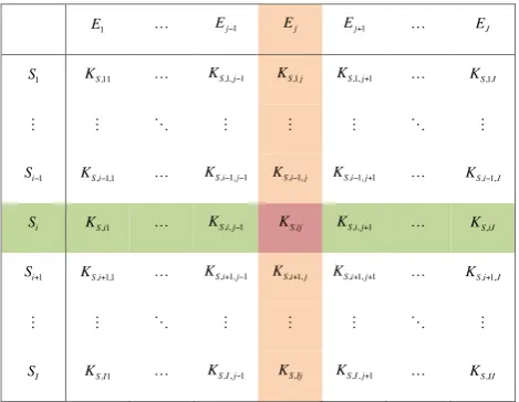
where we have assumed the reaction network includesI sub-strates andJ enzymes (a visualizing way to write Eq. 13 is shown in Fig. 1). By combining Eq. (11) with Eq. (13), this ECA kinetics states that the uptake of substrate Si by

consumerEj depends on (i) the characteristics of the

con-sumer and substrate of interest (throughKS,ij)and (ii) the

characteristics of abiotic and biotic interactions with other substrates and consumers (throughKS,kj andKS,ik). In

par-ticular, when applied to predator–prey systems, the ECA ki-netics indicates that predation rate is neither ratio nor density dependent, a problem that is yet still under debate (Arditi and Ginzburg, 1989; Abrams, 2000; Vucetich et al., 2002; Schenk et al., 2005; Kratina et al., 2009). Next, we derive a few interesting results from Eq. (13).

First, for a reaction that has only one enzyme interacting with one substrate, we have

C11=

S1,TE1,T

KS,11+S1,T+E1,T

, (14)

which is equivalent to Eq. (3). When the substrate concentra-tion is much higher than the enzyme concentraconcentra-tion, such that the microbial process barely changes the total substrate con-centration in the temporal window of interest,KS,11+S1,T

is almost constant, and Eq. (14) becomes the reverse MM ki-netics (Schimel and Wintraub, 2003). When the substrate is changing significantly while the overall enzyme concentra-tion is much lower than the substrate, so thatKS,11+E1,T

is almost constant, Eq. (14) is reduced to the classical MM kinetics (Michaelis and Menten, 1913).

Second, when enzyme concentrations are very high, more inactive enzymes (e.g., transporters of dead cells) will com-pete with the active enzymes for substrate adsorption, conse-quently introducing an inhibition. By treating the active and inactive fractions of an enzyme as two different enzymes, Eq. (14) can be reformulated as

C11=

S1,TE1,T

S1,T+KS,11

1+ E1,T

KS,11+

E2,T

KS,12

, (15)

whereE1,T(mol m−3)andE2,T(mol m−3)are the total

con-centrations of the active and inactive enzymes, respectively. By takingα1as the transient partitioning coefficient between

active and inactive enzyme concentrations (i.e.,E1,T=α1ET

andE2,T=(1−α1) ET, with ET=E1,T+E2,T), Eq. (14)

can be rewritten as

  E1   !   Ej!1   Ej   Ej+1   !   EJ  

S1   KS,11   !   KS,1,j!1   KS,1j   KS,1,j+1   !   KS,1J  

!   !   !   !   !   !   !   !  

Si!1   KS,i!1,1   !   KS,i!1,j!1   KS,i!1,j   KS,i!1,j+1   !   KS,i!1,J  

Si   KS,i1   !   KS,i,j!1   KS,ij   KS,i,j+1   !   KS,iJ  

Si+1   KS,i+1,1   !   KS,i+1,j!1   KS,i+1,j   KS,i+1,j+1   !   KS,i+1,J  

!   !   !   !   !   !   !   !  

SI   KS,I1   !   KS,I,j!1   KS,Ij   KS,I,j+1   !   KS,IJ  

Fig. 1. A matrix-based representation of the parameter

configura-tion for the ECA substrate kinetics (Eq. 13).

C11=

α1S1,TET

S1,T+KS,11 h

1+

α1

KS,11+

1−α1

KS,12

ET

i (16)

= α1S1,TET

S1,T+KS,11

1+ET

KI

,

where KI=

α1

KS,11+

1−α1

KS,12

−1

and the term after the sec-ond equal sign is equivalent to Eq. (2) derived in Suzuki et al. (1989), where they used it to explain the inhibition effect from ineffective binding between substrate and inactive cells. We point out that Eq. (16) could be used to represent the inhi-bition effect from soil minerals, which can compete for sub-strates analogously as an ineffective enzyme (that does not result in a new chemical product but may protect the sub-strates from microbial attack).

Third, for the case of many enzymes competing for a sin-gle substrate, Eq. (13) can be reduced to

C1j=

S1,TEj,T

KS,1j

1+

k=J

P

k=1

Ek,T

KS,1k

+S1,T

. (17)

Grant et al. (1993) used a variant of Eq. (17) to represent the competitive uptake of a substrate in the presence of many mi-crobes (see their Eqs. 3 and 4). However, Grant et al. (1993) directly generalized the results by Suzuki et al. (1989) (with-out explicit derivation) and also implicitly assumed that there are ineffective enzymes competing for substrates. With this latter assumption, Eq. (17) can rewritten as

C1j=

αjS1,TEj,T

KS,1j

1+

k=J

P

k=1

Ek,T

KI,1k

+S1,T

whereαj is the transient active fraction of enzymeEj and

the inhibition constants are KI,1k=

_α

k

KS,1k

+ 1−αk

KS,1k,d

−1

, (19)

whereKS,1k andKS,1k,dare affinity constants of the active

and inactive enzymeEk, respectively. Note that the value of

Jin Eq. (18) is half of that in Eq. (17) since Eq. (18) groups the active and inactive fractions of an enzyme into one.

Fourth, in the case of a single enzyme interacting with many substrates, Eq. (13) is reduced to

Ci1=

Si,TE1,T

KS,i1

1+

k=I

P

k=1

Sk,T

KS,k1

+E1,T

. (20)

WhenE1,Tis constant, Eq. (20) can be equivalently rewritten

as Ci1=

Si,TE1,T

ˆ

KS,i1

1+KS,i1 ˆ

KS,i1

k=I

P

k=1

Sk,T

KS,k1

, (21)

where _Kˆ

S,i1=KS,i1+E1,T. If further assuming KˆS,i1

E1,T, such thatKˆS,i1=KS,i1, then Eq. (21) is just the

multi-component Langmuir isotherm for multimulti-component adsorp-tion in aqueous chemistry (e.g., Choy et al., 2000) and has been used for multi-prey predation in predator–prey mod-els (e.g., Murdoch, 1973). We also note the multicomponent Langmuir isotherm is based on sQSSA.

If there are only two substrates (i.e.,I=2), Eq. (20) can be rewritten as

C11=

S1,TE1,T/KS,11

1+ S1,T

KS,11+

S2,T

KS,21+

E1,T

KS,11

(22a)

C21=

S2,TE1,T/KS,21

1+ S1,T

KS,11+

S2,T

KS,21+

E1,T

KS,21

. (22b)

Then by further assuming E1,T/KS,11 andE1,T/KS,21 are

much smaller than the other terms, one obtains the Eq. (20) in Maggi and Riley (2009). Druhan et al. (2012) have used Eq. (20) by Maggi and Riley (2009) to explain sulfur isotope fractionation in a field subsurface acetate amendment exper-iment. Our Eq. (22) is based on the tQSSA, which makes it valid for a wider range of substrate and enzyme concen-trations. This contrasts our Eq. (22) with Maggi and Riley’s Eq. (20), which is based on the sQSSA, and was found to incorrectly predict isotopic fractionations when enzyme con-centrations were comparable or higher than substrate concen-trations.

2.3 Extension to other inhibitory mechanisms

The EC and ECA kinetics inherently account for competi-tive inhibition (inhibition mechanism (i)), including product

competitive inhibition. For enzyme kinetics or, more broadly, microbe–substrate networks, there are three additional main inhibitory mechanisms often considered (Cornish-Bowden, 1995): (ii) uncompetitive inhibition (inhibitor binds to the enzyme-substrate complex to make the binding ineffective); (iii) noncompetitive inhibition (inhibitor binds equally well to both free enzyme and enzyme-substrate complexes and reduces the number of effective bindings but does not af-fect the enzyme’s substrate affinity); and (iv) mixed inhibi-tion (a mixture of competitive and noncompetitive inhibiinhibi-tion, but the inhibitor has different affinity for free enzyme and the enzyme-substrate complex).

The EC kinetics is compatible with all these four in-hibitory mechanisms, as long as the reaction coefficients can be properly defined for all the inhibitor binding equations. However, the simplified ECA kinetics is only able to repre-sent competitive and noncompetitive inhibition (with some modifications discussed below). Including mixed and non-competitive inhibition is only possible when many substrates are competing for a single enzyme or vice versa (and the relevant mathematics is much more complicated than we have presented for competitive and noncompetitive inhibi-tions here). In addition, as will be demonstrated later (see the numerical experiments), even the ECA kinetics without in-hibitory mechanisms (ii), (iii), and (iv) are not always highly accurate (compared to EC kinetics), nor can they be cali-brated robustly due to parameterization equifinality (i.e., dif-ferent combinations of parameters can result in very simi-lar model predictions (e.g., Beven, 2006; Tang and Zhuang, 2008)). Since including these other inhibitory mechanisms (beside competitive inhibition) will generally introduce more parameters, making the simulations more uncertain, the gain in mechanistic representation is thus smaller than the loss of predictive capability.

Nevertheless, a first order approximation for the noncom-petitive inhibition can be achieved by, first, modifying the substrate affinity coefficients (used in Eq. 13) that are subject to the inhibitorsIk, k=1,· · ·, Las

˜

KS,ij=

KS,ij

k=L

P

k=1

Ik,T

KI,ij k+1

, (23)

whereKI,ij k, k=1, . . . , Lare the inhibition coefficients of

each inhibitor on enzyme-substrate complexCij. In deriving

Eq. (24) we assume that any two inhibitors cannot bind si-multaneously to an enzyme-substrate complex.

Second, substituting the modified substrate affinity coeffi-cientsK˜S,ij into Eq. (13), one obtains the enzyme-substrate

complex concentration (under the influence of noncompeti-tive inhibition):

˜

Cij=

Si,TEj,T

KS,ij

1+

k=I

P

k=1

Sk,T

˜

KS,kj

+

k=J

P

k=1

Ek,T

˜

KS,ik

2.4 Linking with microbial traits

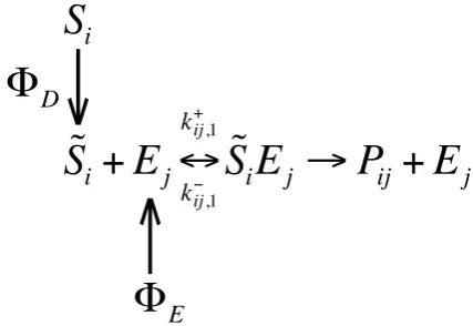
An appealing application of the EC and ECA kinetics is to trait-based modeling of marine and soil microorganisms (Follows et al., 2007; Litchman et al., 2007; Allison, 2012; Bouskill et al., 2012). In the trait-based modeling approach, parameters of the substrate uptake kinetics are determined by the microorganisms’ traits, such as cell size and trans-porter density (e.g., Follows et al., 2007; Armstrong, 2008; Bonachela et al., 2011). Both the EC and ECA kinetics are compatible with such concepts, and the incorporation of these traits can be accomplished efficiently through the dy-namic update of relevant microbial state variables in the nu-merical model. For instance, to consider the effect of cell size (which affects substrate diffusion between the environment and the cell) and transporter density (which affects process-ing rate and affinity to the substrate) on substrate uptake, one has the updated substrate uptake (see diagram shown in Fig. 2). With the stationary flux assumption (Pasciak and Gavis, 1974, 1975), one obtains the diffusive flux to a spher-ical cell as8D=4π Dirc,jnj

Si− ˜Si

, whereDi (m2s−1)

is the diffusivity of the substrateSi in water (when in soil,

this diffusivity depends on soil matric potential, soil struc-ture, and temperature),rc,j (m) is the average size of cellj

(by assuming a spherical cell shape in the first order approxi-mation), andnj(number of cells m−3)is the number density

of cellj. The impact of advection on the flux8Dcan also be

included using the dimensionless Sherwood number (Karp-Boss et al., 1996), but that will not change our derivation essentially. Further assuming the internal substrateS˜i

con-centration (that is close to the cell) is also stationary (thus 8Dis equal to the net enzyme-substrate complex formation

rate betweenS˜i and the cell’s transporter), one obtains (as a

first order approximation)

˜

Si=

4π DircnjSi

k+_ij,1Ej+4π Dircnj

≈ 4π DircnjSi

k_ij,+₁Ej,T+4π Dircnj

, (25)

where we have assumed the reverse dissociation of the enzyme-substrate complex (k_ij,−₁)is negligible, Ej≈Ej,T,

and the changing rate of the enzyme (or transporter) abun-dance due to new growth is much slower than the enzyme-substrate complex equilibration rate. Therefore, one can rep-resent the enzyme-substrate complex with Eq. (7) and a mod-ified equilibrium coefficient:

˜

KS,ij=

k_ij,−₁+k+_ij,2

k+_ij,1 1

+ k

+

ij,1Ej,T

4π Dirc,jnj !

(26)

which leads to a new representation of the substrate affinity parameter for Eq. (13) as

˜

KS,ij=KS,ij 1+

k_ij,+₁Ej,T

4π Dirc,jnj !

. (27)

!

S

_i

+

E

_j

!

k

k

!

S

_i

E

_j

#

P

_ij

+

E

_j

!

S

_i

!

!

_E

!

_D

Fig. 2. Diagram of the updated substrate uptake process, which

in-cludes diffusive substrate flux (between the external environment and near cell environment) and new enzyme production8E. Here

Si is any environmental substrate abundance,S˜iis the correspond-ing local (close to the transporter) substrate abundance, andPij is the assimilated product from the processing ofSiby enzymeEj.

Under the assumption that k_ij,−₁k_ij,+₂ and defining Vmax,ij=k+ij,2Ej,T, one has

˜

KS,ij=KS,ij

1+ Vmax,ij

4π Dirc,jnjKS,ij

, (28)

which extends the modified MM kinetics derived for a single enzyme single substrate system (Bonachela et al., 2011) to an enzyme–substrate network of arbitrary size.

Equation (29) implies that if a cell increases its volumet-ric transporter density (Ej,T/nj; transporters per cell), it

de-creases its substrate affinity. However, considering Ej,T=

njψj4π rc2,j, if a cellj decreases its volumetric size while

keeping the same area-based transporter density ψj

(trans-porters m−2), it can increase its substrate affinity. Further, by substitution of Eq. (28) or Eq. (29) into Eq. (13), one obtains a new representation of the moisture effect on organic matter decomposition (through diffusivityDjand aqueous substrate

concentrationSi)that is more mechanistic than the usually

applied simple multiplier factors (e.g., Andren and Paustian, 1987; Rodrigo et al., 1997; Bauer et al., 2008; Parton et al., 1988).

2.5 Evaluation of the ECA kinetics and the classical MM kinetics

1999) and then compared its predictions to those from the classical MM kinetics and the ECA kinetics for different net-work configurations. We conducted the evaluation with three groups of experiments: (E1) random sampling; (E2) appli-cations to simple microbial models of different complexi-ties; and (E3) simulating litter decomposition with a different carbon-only model. We remark that in all our evaluations all the substrate kinetics used the same number of parameters; therefore, when one formulation is found to perform worse than others, it is inferior in our evaluation framework.

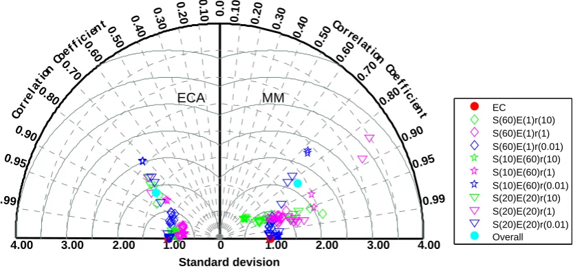
In the first group of experiments (E1; random sampling), we tested the hypothesis that our ECA kinetics is more accu-rate than the MM kinetics for arbitrary consumer–substaccu-rate networks. Specifically, we randomly generated substrate affinity parameters using an exponential distribution over the relative range 1–104 (mol m−3_{), which is sufficiently wide}

to represent the range of microorganisms in the natural envi-ronment (e.g., Wang et al., 2012). The enzymes and substrate concentrations were then generated from the least informa-tive uniform distributionU[0,1]. We performed 9 scenarios using combinations of three substrate : enzyme (SE) ratios (10, 1, and 0.01) and three network sizes (60 substrates and one enzyme, 10 substrates and 60 enzymes, and 20 substrates and 20 enzymes). Each scenario has 10 random replicates, re-sulting in a total of 9×10=90 evaluations. We normalized the variance of the EC solution for each replicate of the 9 sce-narios, and summarized the results using the Taylor diagram (Taylor, 2001), which simultaneously presents the correlation coefficient and root mean square error between the baseline EC solution and solutions using MM or ECA kinetics. Since the equilibrium reaction Eq. (7) is symmetric to represented substrates and enzymes, the 9 scenarios effectively represent 18 different enzyme–substrate networks (e.g., 10 substrates and 60 enzymes is equivalent to 60 substrates and 10 en-zymes). We remark that the high enzyme : substrate ratio may not be ecologically significant for modeling litter decompo-sition such as E3, but it is important to be investigated given our EC and ECA approaches are also applicable for problems such as predator–prey systems, where moderate to high ratio of predator to prey (analogously to that between enzyme and substrate) can easily occur.

In the second group of experiments (E2; simple micro-bial models of different complexities), we used the following generic model structure to illustratively evaluate the impact of different substrate kinetics on microbial system dynamics:

dSi

dt = −

j=J

X

j=1

k_ij,+₂Cij, i=1, . . . , I (29)

dBj

dt =

i=I

X

i=1

µijk_ij,+2Cij−γjBj, j=1, . . . , J, (30)

whereµij (unitless) is the biomass yield rate of microbeBj

(mg C dm−3)from feeding on substrateSi, andγj(day−1)is

respiration rate, which is defined accordingly (in the captions of the relevant parameter tables) for different models. We computedCijusing EC kinetics, MM kinetics (Appendix C),

and ECA kinetics (Eq. 13) and evaluated the ability of the two analytical approximations to reproduce the temporal dy-namics simulated by the EC kinetics. We considered four mi-crobial models of different complexities (Tables 1, 2, and 3; note the fourth model assigned different units to the variables compared to the other three models in order to use the param-eters from Moorhead and Sinsabaugh (2006). We note that using the parameters from Moorhead and Sinsabaugh (2006) is simply a choice of convenience, but it is sufficient for a qualitative assessment of the predicted differences between our ECA or EC-based models and the MM model): (i) three substrates and one microbe (S3B1); (ii) three substrates, one microbe, and one mineral surface (S3B1M1); (iii) one sub-strate and five microbes (S1B5); and (iv) three microbes and three substrates (S3B3). For the three models with three sub-strates (S3B1, S3B1M1, and S3B3), we related the subsub-strates to water-soluble carbon, cellulose, and lignin, respectively. Since the results from (E2) are applicable to other similar problems, we labeled the three substrates asS1,S2, andS3.

For model S1B5, we ran the model with different kinetics using 20 randomly generated parameter sets, and evaluated their performance by the relative model error:

err(t )= 3

N

i=N

X

i=1

yi,EC(t )−yi,app(t )

yi,EC(t )+yi,MM(t )+yi,ECA(t )

, (31)

whereN=6, the number of model state variables, and app refers to MM or ECA. The above metric avoids division by zero as long as the model difference is non-zero.

For all models (including S1B5), we specified the relevant parameter values randomly, but kept their nominal values in the ranges documented in the literature (for microbial param-eters, see Li et al, 1992; Allison et al., 2010; Wang et al., 2012; for mineral adsorption parameters, see Mayes et al., 2012). As an extra comparison, we also included the multi-component Langmuir isotherm (i.e., Eq. 21, which we no-tate as ECA-ML) to compute the substrate uptake in models S3B1, S3B1M1, and S3B3. Since ECA-ML can be derived based on sQSSA and it assumes enzyme concentrations are much lower than the substrate concentrations, comparing its performance with that of ECA and EC will reveal the advan-tage of tQSSA in representing networks with high enzyme concentrations.

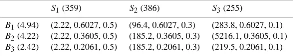
Table 1. Parameter values for microbial models S3B1 and S3B1M1.

The parameter vectors are presented in the form

KS,ij, k+_ij,2, µij

,

whose units are, respectively, mg C dm−3, d−1, and none. The ini-tial microbial biomass is defined in the parentheses afterB1, whose

unit is mg C dm−3. The mineral surface is characterized with the Langmuir dissociation parameter (equivalentlyKS,ij)and the max-imum adsorption capacity (in the parentheses followingM1), whose

units are, respectively, mg C dm−3and mg C dm−3. For both mod-els, we used a microbial respiration rate 0.03 d−1. The microbial parameters were randomly specified based on prior knowledge from Wang et al. (2012), and the mineral surface parameters were speci-fied for Alfisol based on Mayes et al. (2012).

S1(30) S2(100) S3(90)

B1(0.1) (1, 48, 0.5) (10, 48, 0.3) (50, 48, 0.1)

M1(1094) (21.2, 0, 0) (21.2, 0, 0) (21.2, 0, 0)

Table 2. Parameter ranges for microbial model S1B5. The

param-eter vectors are presented in the formKS,ij, k+_ij,2, µij

, whose

units are, respectively, mg C dm−3, d−1, and none. Numbers in the parentheses following the state variables are their initial values, whose units are mg C dm−3. All five microbes used a respiration rate 0.005 d−1. The maximum and minimum parameter values were specified based on Wang et al. (2012).

S1(300)

Minimum Maximum values values

B1(1) (1, 1, 0.4) (100, 10, 0.4)

B2(1) (1, 1, 0.4) (100, 10, 0.4)

B3(1) (1, 1, 0.4) (100, 10, 0.4)

B4(1) (1, 1, 0.4) (100, 10, 0.4)

B5(1) (1, 1, 0.4) (100, 10, 0.4)

approximating the EC solution; and (ii) only the ECA kinet-ics is analytically tractable and sufficiently accurate to model microbial–mineral surface interactions.

For the third set of experiments (E3; simulating litter de-composition), we tested whether the S3B3 model with dif-ferent substrate kinetics can be calibrated to simulate the 77-month red pine litter decomposition data of Melillo et al. (1989). We first calibrated model S3B3 with both the ECA and MM kinetics, and analyzed if the calibrated models can reproduce the (i) two-phase evolution of remaining or-ganic matter, (ii) increase of lignocellulose index (LCI) dur-ing decomposition, and (iii) reasonable fraction of microbial biomass with respect to the remaining organic matter. We then ran the models with 9 different initial litter chemistries (Table 4) for a qualitative assessment of the extrapolated pre-dictability (based on observational data if available) of the calibration. We were able to obtain some time series data for the Massachusetts (MA) site (Magill et al., 1998), but failed to extract any useful time series data for the Wisconsin (WI)

Table 3. Prior parameters for microbial model S3B3. The parameter

vectors are presented in the formKS,ij, kij,+2, µij

, whose units

are, respectively, g C, d−1and none. All values are adapted from Moorhead and Sinsabaugh (2006). All three respiratory coefficients (i.e.,γj, j=1,2,3 as defined in Eq. (30) are set to 0.03 d−1. Num-bers in the parentheses following the state variables are their initial values, whose units are g C.

S1(448) S2(431) S3(121)

B1(0.33) (1, 1, 0.5) (100, 1, 0.3) (5000, 1, 0.1)

B2(0.33) (1.0, 0.8, 0.5) (10, 0.8, 0.3) (1000, 0.8, 0.1)

B3(0.33) (1.0, 0.4, 0.5) (10, 0.4, 0.3) (100, 0.4, 0.1)

Table 4. Characteristics of initial litter chemistry for the data in

litterbag decomposition field studies in Wisconsin (WI) and Mas-sachusetts (MA). The table is organized based on Table 3 in Moor-head and Sinsabaugh (2006), who obtained data from Aber et al. (1984) and Magill et al. (1998). The final LCI is model predicted (see Sect. 3.3.2 for details). We have also extracted time series data from the Magill et al. (1998) study for model assessment (Figs. 15 and S1).

Litter type, Labile Holocellu- Lignin Initial Final by site (%) lose (%) (%) LCI LCI

Wisconsin (WI)

Sugar maple 44.8 43.1 12.1 0.22 0.55

Aspen 31.1 47.5 21.4 0.31 0.56

White oak 32.4 47.4 20.2 0.30 0.56 White pine 32.8 44.7 22.5 0.33 0.59 Red oak 30.0 45.2 24.8 0.35 0.59

Massachusetts (MA)

Red pine 35.9 38.6 25.5 0.40 0.67 Red maple 47.7 35.4 16.9 0.32 0.68 Black oak 35.0 39.6 25.4 0.39 0.66 Yellow birch 43.4 40.3 16.3 0.29 0.62

site (Aber et al., 1984) from the original literature or by con-tacting the authors. In addition, we noticed the original data in Magill et al. (1998) indicated a rise of lignin during the de-composition for some unexplained reasons (see their Fig. 4). We corrected this by replacing the unreasonable lignin data (i.e., those higher than the initial lignin mass) with the initial lignin mass (see Fig. S1 for details).

Table 5. Best-fit parameters for model S3B3-ECA by optimizing the simulation outputs to the 77-month red pine litter decomposition

experiment data in Melillo et al. (1989). The parameter vectors are presented in the formKS,ij, kij,+2, µij

, whose units are, respectively,

g C, d−1, and none. The respiratory coefficients (i.e.,γj, j=1,2,3 as defined in Eq. (31) of the three microbes are, respectively, set to 0.01, 005, and 0.001 d−1. Numbers in the parentheses following the state variables are their initial values, whose units are g C. In doing the calibration, we assumed (i)KS,1j, j=1,2,3 are same for all three microbes; (ii)KS,22=KS,23; (iii) for microbeBj,kij,+2, i=1,2,3 are

same for all three substrates. By further fixingµijto the values in the parentheses, we effectively had a total 12 parameters in the calibration.

S1(359) S2(386) S3(255)

B1(4.94) (2.22, 0.6027, 0.5) (96.4, 0.6027, 0.3) (283.8, 0.6027, 0.1)

B2(4.22) (2.22, 0.3605, 0.5) (185.2, 0.3605, 0.3) (5216.1, 0.3605, 0.1)

B3(2.42) (2.22, 0.2061, 0.5) (185.2, 0.2061, 0.3) (219.5, 0.2061, 0.1)

that for model S3B3 runtime was 1500 days. All models in experiment E3 were run for the length of the observations (80 months).

Bayesian inference based calibrations for experiment E3 were performed to invert the relevant parameters (see cap-tion of Table 5 for descripcap-tions) of the substrate uptake ki-netics from fitting the model (e.g., S3B3-ECA) output to the time series data of the remaining litter mass and ligno-cellulose index (LCI) from Melillo et al. (1989). We imple-mented the Bayesian inference using the MCMC algorithm DREAM (Vrugt et al., 2008). A uniform prior was used for all the parameters, with the cost function (or the negative log-likelihood function) defined by

Jcost=(8σLCI)−1

k=8

X

k=1

LCIk−LCIECA,k

(32)

+(17σMass)−1

k=17

X

k=1

rMass,k−rMass,ECA,k

,

where LCIkis thekth observation of lignocellulose index (of

which there are 8 data points) andrMass,kis thekth

observa-tion of relative remaining organic matter biomass (microbe plus litter; of which there are 17 data points). BothσLCIand

σMass are set to 0.01. For the posterior parameters, the set

that minimizesJcostis defined as the modal (i.e., best fitting)

parameter.

3 Results and Discussion

3.1 E1: computing enzyme-substrate complexes for

large networks

For the first set of experiments, we found that ECA kinetics performed better or as well as MM kinetics in approximat-ing the baseline EC solutions. When the substrate to enzyme ratio was high (i.e., enzyme availability is limiting decompo-sition; green symbols in Fig. 3), the ECA solutions agreed with the EC solutions with correlation coefficients higher than 0.95 and root mean square errors less than 0.5 standard deviations (σ), except for 2 (out of 10) random replicates

for caseS(60)E(1)r(10) (i.e., 60 substrates, 1 enzyme, and a substrate to enzyme abundance ratio of 10; similar nomen-clature is used henceforth) and 3 (out of 10) replicates for case S(20)E(20)r(10), whose correlation coefficients were still good (∼0.80) and the corresponding root mean square errors were between 0.5σ and 1.5σ.

MM kinetics also achieved good accuracy in approximat-ing the EC solution with correlation coefficients between 0.75 and 0.97, but in general higher root mean square er-rors. For caseS(10)E(60)r(10), MM kinetics only achieved a correlation coefficient of 0.80 and root mean square er-rors greater than 0.5σ, whereas ECA kinetics achieved cor-relation coefficients of ∼0.99 and root mean square errors smaller than 0.3σ. However, the worst approximations (in terms of root mean square error) by the MM kinetics (i.e., two replicates, green diamond symbols, forS(60)E(1)r(10)) were better than those from the ECA kinetics (for these two poorly simulated replicates).

Similarly contrasting results were found for the cases when the substrate to enzyme ratio was one (purple symbols in Fig. 3): (i) the best approximation by the ECA kinetics was better than that using the MM kinetics and (ii) the MM kinetics resulted in 2 outliers for the case S(20)E(20)r(1) with root mean square errors greater than 2σ and correla-tion coefficients less than 0.90. ECA kinetics also produced 4 random replicates (2 for case S(10)E(60)r(1) and 2 for caseS(20)E(20)r(1)) that had correlation coefficients close to 0.8, but the root mean square error was less than 1.5σ.

When substrate was limiting (blue symbols), both the ECA and MM kinetics produced poor approximations (with more outliers) compared to the EC solutions. Both approaches pro-duced 4 outliers (2 for caseS(10)E(60)r(0.01) and 2 for case S(20)E(20)r(0.01)) with correlation coefficients between 0.70 and 0.80 and root mean square errors greater than 1σ. The worst results (the 2 replicates forS(20)E(20)r(0.01)) by MM kinetics were again worse than those by ECA kinetics.

Co

rre_{l a}

t io_n

C_oe ff_ic

ie_n t Corr

ela

t ion

Coe ffic

ient

0.10 0.20 _0.30

0.40

0.50

0.60

0.70

0.80

0.90

0.95

0.99

0.10 0.20

0.30 0.40 0.50 0.60

0.70

0.80

0.90

0.95

0.99

0.0

0

Standard devision 1.00

1.00 2.00

2.00 3.00

3.00 4.00

4.00

ECA MM

EC

S(60)E(1)r(10) S(60)E(1)r(1) S(60)E(1)r(0.01) S(10)E(60)r(10) S(10)E(60)r(1) S(10)E(60)r(0.01) S(20)E(20)r(10) S(20)E(20)r(1) S(20)E(20)r(0.01) Overall

Fig. 3. A Taylor diagram based summary of the random sampling experiment (E1) that compared the ability of the ECA and the MM kinetics

to approximate different enzyme–substrate networks simulated by the EC kinetics. Each symbol has 10 random replicates. The values in the parentheses indicate the number of substrates or enzymes. The nomenclatureS(x)E(y)r(z) indicate a network ofxsubstrates,yenzymes, and a substrate to enzyme abundance ratio ofz.

kinetics is superior to the MM kinetics in representing large-size consumer–substrate networks.

3.2 E2: application to simple microbial models

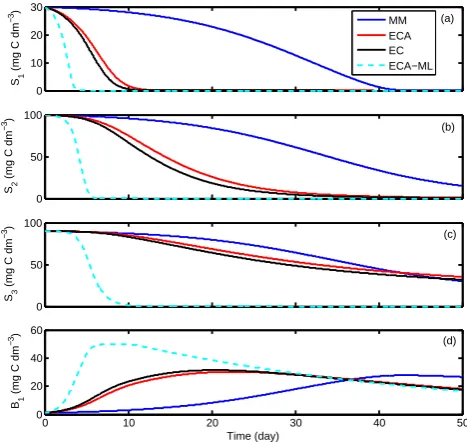
We found three (EC, ECA, ECA-ML) of the four different substrate kinetics led to almost identical model predictions for the S3B1 scenario over the 50-day time period (Figs. 4 and 5). The MM predictions deviated from the others slightly. However, the good agreement between the MM kinetics and the other kinetic formulations is serendipitous. The MM ki-netics is poor in describing enzyme competition in the pres-ence of multi-substrates, which has been identified in several studies (e.g., Maggi and Riley, 2009; Druhan et al., 2012). We also replicated this behavior with an isotope-modeling example (see Supplement), where it was shown the MM ki-netics has very poor predictability for multi-isotopic fraction-ations (Fig. S3), even though it predicted the bulk substrate and microbial dynamics with acceptable accuracy (Fig. S2).

When mineral surface interactions were further included (in the S3B1 model) to form the S3B1M1 model, we found that the ECA kinetics again predicted very similar time se-ries compared to that from EC kinetics (Figs. 6 and 7) be-cause both ECA and EC are able to consistently represent the substrate competition by microbe and mineral surfaces. However, both the ECA-ML and MM kinetics resulted in predictions substantially different from the EC solution. The ECA-ML predicted a much faster turnover rate of all three substrates because it did not include the inhibitory term due to the presence of consumers (which can be confirmed by comparing Eq. 13 to Eq. 21) and thence resulted in a

0 50 100

S3

(mg C dm

−

3)

(c) 0

50 100

S2

(mg C dm

−

3)

(b) 0

10 20 30

S1

(mg C dm

−

3)

(a)

0 10 20 30 40 50

0 20 40 60

Time (day) B1

(mg C dm

−

3)

(d) MM

ECA EC ECA−ML

Fig. 4. Time series of the relevant state variables simulated from

the applications of the four different substrates uptake kinetics to microbial model S3B1.

0.4 0.6 0.8 1

LCI

(b) 0

20 40 60 80 100

Remaining litter (%)

(a)

0 10 20 30 40 50

0 0.2 0.4 0.6 0.8 1

Fractional of microbial C

Time (day)

(c) MM

ECA EC ECA−ML

Fig. 5. Time series of state variable ratios simulated from the

appli-cation of the four different substrates uptake kinetics to microbial model S3B1.

because (by comparing Eq. C1 to Eq. 13) it did not in-clude the nonlinear competitive inhibition on substrate up-take or the inhibition due to the presence of the consumer. In addition, the mineral adsorption sites (counted as adsorp-tion capacity by the state variableM1 in Table 1) is much

more abundant than microbial transporters, which resulted in a strong limitation on microbial substrate uptake. This sub-strate limitation (due to mineral surface adsorption) led to a much lower microbial growth, which then led to a greatly underestimated substrate turnover rate (by the MM kinetics). Therefore, the reduction in turnover of the three substrates in presence of mineral surface adsorption leads us to con-jecture that mineral adsorption (and consequently protection, which is not considered here but can be incorporated by us-ing approaches such as in Wang et al., 2013) is an impor-tant mechanism impacting organic matter degradation with depth in the soil profile. Implementing the ECA or EC ki-netics could thus potentially avoid the ad hoc parameteriza-tion of soil organic matter (SOM) decomposiparameteriza-tion rate slow-down with depth, as has been implemented in some verti-cally resolved SOM models (e.g., Jenkinson and Coleman, 2008; Koven et al., 2013). In accordance with the predicted substrate dynamics, we note that MM kinetics predicted the slowest increase in LCI and fractional microbial C (with re-spect to total organic C including both substrates and mi-crobial biomass), while the ECA-ML kinetics predicted the fastest increase (Fig. 7). These findings lead us once again to state that the MM kinetics is qualitatively not appropriate when the problem involves multiple substrates and multiple

0 50 100

S3

(mg C dm

−

3) _(c)

0 50 100

S2

(mg C dm

−

3) _(b)

0 10 20 30

S1

(mg C dm

−

3) _(a)

0 10 20 30 40 50

0 20 40 60

Time (day) B1

(mg C dm

−

3) _(d)

MM ECA EC ECA−ML

Fig. 6. Time series of the relevant state variables simulated from

the applications of the four different substrate uptake kinetics to microbial model S3B1M1.

0.4 0.6 0.8 1

Litter LCI

(b) 0

20 40 60 80 100

Remaining litter (%)

(a)

0 10 20 30 40 50

0 0.2 0.4 0.6 0.8 1

Fraction of microbial C

Time (day)

(c) MM

ECA EC ECA−ML

Fig. 7. Time series of state variable ratios simulated from the

appli-cation of the four different substrates uptake kinetics to microbial model S3B1M1.

consumers. In addition, as we will show in experiment E3, such deficiencies cannot be remedied through calibration.

0 20 40 60 80

(e) B₄

(mg C dm

−

3)

0 20 40 60

(f) B 5 0.9

1 1.1

(c) B 2

(mg C dm

−

3)

0 5 10

(d) B 3 0

100 200 300

(a) S 1

(mg C dm

−

3)

1 1.2 1.4

(b) B 1

0 10 20 30 40 50

0 0.2 0.4 0.6

(g) Err−MM

Time (day)

0 10 20 30 40 50

0 0.2 0.4 0.6

(h) Err−ECA

Time (day) MM ECA EC

Fig. 8. Comparison of simulations using different substrate kinetics

in scenario S1B5: (a–f) are from the simulation that showed the most distinctive differences; (g) and (h) are summaries of the model differences (with respect to the EC results) from the ensemble of 20 random simulations.

metrics defined in Eq. 32) among the 20 runs with randomly generated parameters (see Table 2 for parameters being sam-pled), the prediction by the MM kinetics fit the EC predic-tions better than did the ECA kinetics (Fig. 8a–f). When sum-marized over the 20 runs (Fig. 8g–h), we found that the MM kinetics is slightly superior for problems that are in the form of many microbes competing for a single substrate. This re-sult is consistent with model rere-sult such as that in Bouskill et al. (2012), where the ammonia and nitrite oxidizers have a very weak overlap in substrates. However, if one tries to use isotopic data to improve the parameterization of such models, the MM kinetics should be replaced with the ECA kinetics or the EC kinetics.

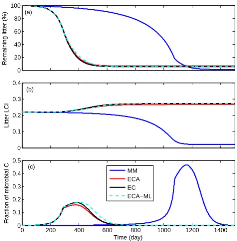
For model S3B3, three of the four substrate kinetics (ECA-ML, ECA, and EC) made very similar predictions (see Figs. 9 and 10). The predictions from the MM kinet-ics were completely different, both qualitatively and quanti-tatively. The MM kinetics predicted a gradual reduction in LCI (which stabilized at a constant value smaller than the initial value; see Fig. 10b), whereas the other kinetic mod-els predicted a gradual increase in LCI, which stabilized at a greater (than the initial) value. In addition, the MM ki-netics predicted a much higher peak fractional total micro-bial biomass (compared to the total biomass accounting for both litter and microbes) than did the other substrate kinetics (Fig. 10c). We note that ECA-ML, ECA, and EC all predicted similar temporal evolutions of the remaining litter and lit-ter LCI that qualitatively agreed with findings from litlit-terbag

0 2 4

B2

(g C)

(e) 0 50 100

B1

(g C)

(d) 0 200 400 600

S3

(g C)

(c) 0 200 400 600

S2

(g C)

(b) 0 200 400 600

S1

(g C)

(a)

0 200 400 600 800 1000 1200 1400

0 0.2 0.4

Time (day) B3

(g C)

(f)

MM ECA EC ECA−ML

Fig. 9. Time series of relevant state variables simulated from the

application of different substrate kinetics to microbial model S3B3.

0 0.1 0.2 0.3 0.4

Litter LCI

(b) 0 20 40 60 80 100

Remaining litter (%)

(a)

0 200 400 600 800 1000 1200 1400

0 0.1 0.2 0.3 0.4 0.5

Time (day)

Fraction of microbial C

(c)

MM ECA EC ECA−ML

Fig. 10. Time series of state variable ratios simulated from the

ap-plication of the four different substrates uptake kinetics to microbial model S3B3.

decomposition is important to represent measured litter dy-namics. Once this nonlinear competition is accounted for, the observed temporal evolution of LCI (and consequently lignin degradation) emerges from the proposed model (EC and ECA). On the other hand, MM kinetics is not structured to account for such nonlinear competition, thus one has to enforce an otherwise unconstrained lignin shielding effect on cellulose degradation (though we do not rule out its possible existence) to make the model well behaved (e.g., Moorhead and Sinsabaugh, 2006; Allison, 2012).

3.3 E3: simulating litter carbon decomposition

3.3.1 Calibrating model S3B3 with different substrate kinetics

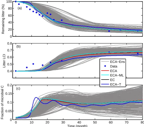
After calibrating the S3B3-ECA model (model S3B3 imple-mented with ECA; same nomenclature are used henceforth) to the 77-month red pine litterbag experiment data, we found the posterior best-fit parameters led to predictions in good agreement with the measured time series of remaining lit-ter and LCI (Fig. 11). The poslit-terior microbial biomass also seemed qualitatively reasonable, which stayed below 15 % of total organic carbon (including both litter and microbial biomass). Observational data indicate the fractional micro-bial biomass is relatively low, usually within 10 % of the total organic carbon (Ladd et al., 1994; Dilly and Munch, 1996). Therefore, considering the parameterization equifinality due to insufficient observational data to constrain the relevant pa-rameters (e.g., Tang and Zhuang, 2008) and the qualitatively good agreement between posterior simulations and the avail-able data, we conclude that ECA kinetics is a better choice than MM kinetics in our parsimonious framework to repre-sent litter decomposition dynamics.

We also ran the S3B3 model with the ECA-ML and EC ki-netics using the same parameters obtained from S3B3-ECA model calibration and obtained almost identical predictions (see red and cyan lines in Fig. 11). As a sensitivity test, we further introduced the temperature effect on substrate up-take (labeled as ECA-T in Figs. 11 and 13) by applying three different Q10 values (whose values are, respectively, 2.7, 1.5, and 1.7 based on Bayesian inversion on top of the default S3B3-ECA model calibration) to the three biomass yield rates. We found the predictions (blue lines in Fig. 11) changed slightly compared to the simulations without ac-counting for temperature effects. Though the Q10 values are quite uncertain because of data limitations, the result indi-cates that temperature was not the single mechanism that led to the differences between measurement and posterior model prediction. Other mechanisms such as leaching, nutrient dy-namics, and moisture effects should be investigated in future studies to improve the EC and ECA litter decomposition ki-netics.

Calibrating the model with the Michaelis–Menten kinet-ics (S3B3-MM) to the 77-month litterbag data failed to

ob-0.4 0.5 0.6 0.7 0.8

Litter LCI

(b) 0 20 40 60 80 100

Remaining litter (%)

(a)

0 10 20 30 40 50 60 70 80

0 0.05 0.1 0.15 0.2

Time (month)

Fraction of microbial C

(c)

ECA−Ens Data ECA ECA−ML EC ECA−T

Fig. 11. Posterior simulations from calibrating model S3B3-ECA

to the red pine litter decomposition experimental data in Melillo et al. (1989). ECA-Ens indicates the posterior ensemble simulations, and ECA-T indicates the additional temperature impact on top of ECA (i.e., the best fitting posterior simulation). The best-fit kinetic parameters for ECA, EC, ECA-ML, and ECA-T are in Table 5. See text for further details.

tain reasonable posterior predictions of the litter decomposi-tion dynamics (Fig. 12). A few parameter combinadecomposi-tions led to qualitatively reasonable predictions of the two-phase evo-lution of remaining biomass and the increasing, then stabi-lizing behavior of LCI. Yet the fractional microbial biomass varied wildly. Many parameter combinations predicted the total biomass as microbial-C dominated (almost 100 %) dur-ing the second phase of litter decomposition. We also found the model S3B3-MM is much more sensitive to the parame-ters than the models implementing ECA-ML, ECA, and EC kinetics. Therefore, we conclude that MM kinetics is not suit-able for modeling microbial litter decomposition and SOM dynamics in our more parsimonious framework (than other existing models), since these problems always involve multi-ple substrates and multimulti-ple microbes.

3.3.2 The interaction between litter chemistry and microbial diversity

0.2 0.4 0.6 0.8 1

Litter LCI

(b) 0 20 40 60 80 100

Remaining litter (%)

(a)

0 10 20 30 40 50 60 70 80

0 0.2 0.4 0.6 0.8 1

Time (month)

Fraction of microbial C

(c)

MM−Ens Data MM

Fig. 12. Posterior S3B3-MM simulations by calibrating the model

to the 77-month red pine litterbag experimental data in Melillo et al. (1989). MM-Ens indicates the posterior ensemble simulations. The best-fit posterior simulation is in red, whose corresponding pa-rameters are in Table S2.

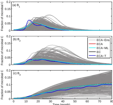
fungal : bacterial ratio in their long-term (730 days) litter de-composition experiment. Considering that fungi often domi-nate lignin decomposition (Osono, 2007), our predicted dom-inance of the fungi-like microbe in the second phase of the 77-month decomposition is qualitatively reasonable. Never-theless, a comprehensive assessment should use a model that has a complete representation of the relevant nutrient dy-namics (e.g., N and phosphorus) and such a model should be compared to detailed observational characterization of lit-ter chemistry and microbial community structure. However, detailed observational characterization of both substrate and microbial community structure is lacking in long-term exper-iments that cover temporal scales varying from diurnal cycles to multiple years. These types of observations are critical to the development of the types of models discussed here.

Considering each member of the posterior ensemble sim-ulation as a single red pine litter decomposition exper-iment with a different microbial community, our results (Figs. 11 and 13) indicate that the evolution of litter chem-istry is strongly regulated by microbial community structure. In addition, parameterization equifinality (see gray lines in Figs. 11 and 13) indicate different microbial communities will sometimes lead to similar litter chemistry after a rel-atively long time. The latter is manifested as a weak con-vergence of litter chemistry in terms of LCI throughout the 77-month period (Fig. 11b; also see the review about mea-surements in Melillo et al., 1989). Yet we found that the

fi-0 0.05 0.1 0.15 0.2

Fraction of microbial C

(b) B 2 0 0.05 0.1 0.15 0.2

Fraction of microbial C

(a) B 1

0 10 20 30 40 50 60 70 80

0 0.05 0.1 0.15 0.2

Time (month)

Fraction of microbial C

(c) B 3

ECA−Ens ECA ECA−ML EC ECA−T

Fig. 13. Simulated time series of microbial abundances from using

the best-fit parameters (calibrated with S3B3-ECA) in Table 5. The four models ECA, ECA-ML, EC, and ECA-T used the same kinetic parameters. The ECA-Ens simulations correspond to the ensemble simulations in Fig. 11.

nal, seemingly constant LCI is not a single value but rather a range between 0.6 and 0.8 for the red pine litter being mod-eled here.

When we applied the model S3B3-ECA using the best-fit parameters (Table 5) from the Bayesian calibration to 9 dif-ferent litter types (Table 4), the results (Fig. 14) indicated a clear dependence of litter decomposition on initial litter chemistry. The predictions indicate all 9 litters were degraded in two phases, and their LCIs rose asymptotically to different final constant values. Furthermore, the final constant LCI is a function of both its initial value and the microbial community diversity and dynamics. For instance, the red maple started with a medium initial LCI (0.32) but reached a final value of 0.68, the highest among the 9 litters (Table 4). While we failed to obtain sufficient data to evaluate the 9 predictions, the evaluation of the 4 litter types in the study by Magill et al. (1998) indicated our model predictions were qualitatively reasonable (Fig. 15). We also applied the Michaelis–Menten kinetics model (S3B3-MM) with its best-fit parameter (Ta-ble S2) to the 9 litter types; its prediction was again poor (see Fig. S5).

0.2 0.4 0.6 0.8

Litter LCI

(b) 0 50 100

Remaining litter (%)

(a)

0 10 20 30 40 50 60 70 80

0 0.1 0.2 0.3 0.4

Time (month)

Fraction of microbial C

(c)

Sugar maple Aspen White oak White pine Red oak Red pine Red maple Black oak Yellow birch

Fig. 14. Model (S3B3-ECA) predicted temporal evolution of litter

decomposition dynamics for the 9 different litters in Table 4. The used parameters are in Table 5.

0 10 20 30 40 50 60 70 80 90 100 0

10 20 30 40 50 60 70 80 90 100

y=0.69x+21.33, R2_=0.87

Measured remaining litter (%)

Predicted remaining litter (%) (a)

0 0.1 0.2 0.3 0.4 0.5 0.6 0.7 0.8 0.9 1 0

0.1 0.2 0.3 0.4 0.5 0.6 0.7 0.8 0.9 1

y=0.58x+0.22, R2_=0.78

Measured LCI

Predicted LCI (b)

Red pine Red maple Black oak Yellow birch

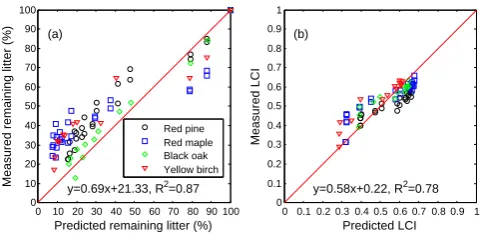
Fig. 15. Evaluation of model (S3B3-ECA) prediction using Magill

et al. (1998) litterbag experiment data: (a) remaining litter biomass and (b) litter lignocellulose index (LCI). The original and corrected lignin data are in Fig. S1.

models such as TEM (McGuire et al., 1997), CENTURY (Parton et al., 1988), and Roth-C (Jenkinson and Coleman, 2008), which implicitly assumed the relevant microbial com-munity structures are constant.

3.3.3 The emergent lignin decomposition dynamics

Lignin dynamics play a critical role in litter decomposition (Berg et al., 1982; Melillo et al. 1982; Machinet et al., 2011). The physically reasonable prediction by model S3B3-ECA provided us with some new insights on lignin decomposi-tion. We found (Fig. 16) that lignin decomposition does not follow the conceptual model proposed by Berg and Staaf (1980), which states that no lignin will be degraded until it reaches a threshold concentration (with respect to the total litter). Rather, our predictions support the conceptual model of Klotzbucher et al. (2011), which states that lignin decom-position depends on the availability of easily degradable la-bile carbon. However, our results add further insights that,

0 20 40 60 80

0 10 20 30 40 50 60 70 80 90 100

Time (month)

Remaining fraction (%)

Sugar maple litter Aspen litter White oak litter White pine litter Red oak liter Red pine litter Red maple litter Black oak litter Yellow birch litter Sugar maple lignin Aspen lignin White oak lignin White pine lignin Red oak lignin Red pine lignin Red maple lignin Black oak lignin Yellow birch lignin

Fig. 16. Model (S3B3-ECA) predicted temporal patterns of total

litter and lignin degradation for the 9 different litter types.

besides litter chemistry, degradation is also regulated by crobial community structure. When different groups of mi-crobes are degrading the same type of litter, the litter chem-istry could evolve differently (e.g., Fig. 11). We note that lignin decomposition is also regulated by nutrient dynamics such as the nitrogen availability (Herman et al., 2008), which will be explored in our follow up studies.

3.4 Potential improvements to the EC and ECA

substrate kinetics for modeling microbial systems

Substrate uptake is a process regulated by many biotic and abiotic factors. For soil microbial systems, relevant abiotic factors are soil moisture, temperature, mineralogy, aggre-gation, and redox potentials (e.g., Davidson and Janssens, 2006). As we explained in Sect. 2.1, EC kinetics allow a direct and consistent description of these abiotic processes using the existing knowledge of reactive transport modeling (Jennings et al., 1982; Jin and Bethke, 2007). Incorporating these factors within the ECA kinetics is more difficult. How-ever, besides the diffusion limitation (which partly accounts for the soil moisture effect as we discussed in Sect. 2.1), accounting for the temperature effect in ECA kinetics is straightforward by recognizing that all parameters in Eq. (4) are temperature dependent. For instance, by using Eyring’s transition state theory (Eyring, 1935a, b), it can be shown thatKS,ij∝exp(−1H /RT ), where1H(J mol−1) is an

ac-tivation energy that should be deducible from measurements (as was done in Davidson et al. (2012), though there they assumedKS,ij was a linear function of temperature).