www.ann-geophys.net/34/473/2016/ doi:10.5194/angeo-34-473-2016
© Author(s) 2016. CC Attribution 3.0 License.
Hydromagnetic waves in a compressed-dipole field via field-aligned
Klein–Gordon equations
Jinlei Zheng1, Qiang Hu1,2, Gary M. Webb2, and James F. McKenzie2,3,† 1Department of Space Science, University of Alabama, Huntsville, AL, USA
2Center for Space Plasma and Aeronomic Research (CSPAR), University of Alabama, Huntsville, AL, USA 3Department of Mathematics and Statistics, Durban University of Technology, Steve Biko Campus,
Durban, South Africa †deceased
Correspondence to: Qiang Hu ([email protected])
Received: 1 November 2015 – Revised: 5 April 2016 – Accepted: 19 April 2016 – Published: 2 May 2016
Abstract. Hydromagnetic waves, especially those of fre-quencies in the range of a few millihertz to a few hertz ob-served in the Earth’s magnetosphere, are categorized as ultra low-frequency (ULF) waves or pulsations. They have been extensively studied due to their importance in the interaction with radiation belt particles and in probing the structures of the magnetosphere. We developed an approach to examining the toroidal standing Aflvén waves in a background magnetic field by recasting the wave equation into a Klein–Gordon (KG) form along individual field lines. The eigenvalue so-lutions to the system are characteristic of a propagation type when the corresponding eigenfrequency is greater than a crit-ical frequency and a decaying type otherwise. We apply the approach to a compressed-dipole magnetic field model of the inner magnetosphere and obtain the spatial profiles of rel-evant parameters and the spatial wave forms of harmonic oscillations. We further extend the approach to poloidal-mode standing Alfvén waves along field lines. In particular, we present a quantitative comparison with a recent space-craft observation of a poloidal standing Alfvén wave in the Earth’s magnetosphere. Our analysis based on the KG equa-tion yields consistent results which agree with the spacecraft measurements of the wave period and the amplitude ratio be-tween the magnetic field and electric field perturbations. Keywords. Electromagnetics (wave propagation) – magne-tospheric physics (magnemagne-tospheric configuration and dynam-ics) – space plasma physics (experimental and mathematical techniques)
1 Introduction
Hydromagnetic waves are common phenomena in space plasmas. The associated magnetic and electric field perturba-tions are observed both on the ground and from space in the Earth’s magnetosphere. Such waves or magnetic pulsations of frequencies less than ∼1 Hz are typically categorized as ultra low-frequency (ULF) waves (Fraser, 2006; Kivel-son, 2006). They can be further divided into subcategories, such as Pc1-5, Pi1-3 and Pg, with frequencies ranging from a few hertz down to a few millihertz (Fraser, 2006; Volw-erk, 2006). Sometimes they exhibit regular and monochro-matic magnetic and electric field wave forms which are due to the standing wave mode along magnetic field lines. Such waves can be identified as Alfvén waves propagating in the Earth’s magnetosphere, e.g., the recent spacecraft observa-tion by the Van Allen Probes (Radiaobserva-tion Belt Storm Probes) of Dai et al. (2013). Based on the direction or the polariza-tion of the magnetic (or electric) field perturbapolariza-tion in the linearized assumption, they can be further characterized as toroidal and/or poloidal-mode waves. In the toroidal mode, the magnetic field perturbation is in the azimuthal direction, i.e., along the east–west longitudinal direction (the accom-panying electric field perturbation has a radial component) in Earth’s dipole magnetic field. On the other hand, in the poloidal mode, the magnetic field perturbation has a radial component, lying in the meridional plane, while the electric field perturbation is azimuthal.
developed. These waves are interpreted as standing Alfvén (transverse) or fast-mode hydromagnetic waves in cold plas-mas immersed in the Earth’s magnetic field (Cummings et al., 1969; Singer et al., 1981; Southwood and Hughes, 1983). Their characteristics are closely governed by the ge-ometry of the background magnetic field and the associated plasma density distribution. More general and sophisticated numerical simulations were also developed in recent years to take into account more realistic background field topology, multiple physical effects and non-idealized boundary condi-tions (Kabin et al., 2007; Lee and Takahashi, 2006; Claude-pierre et al., 2010; Degeling et al., 2010). The study of ULF waves has important implications for wave–particle interac-tion and diagnostics of magnetospheric structures. In partic-ular, the critical role that ULF waves play in the energization and transport of radiation belt particles has been established based on both theoretical and observational studies (Elking-ton, 2006; Elkington et al., 2003, 1999; Takahashi et al., 2002; Ukhorskiy et al., 2005; Dimitrakoudis et al., 2015).
An alternative approach to describing the toroidal (trans-verse) Alfvén standing waves in an axisymmetric back-ground magnetic field has been given by McKenzie and Hu (2010), where the wave equations were cast along an indi-vidual field line and transformed into a Klein–Gordon (KG) form. This approach was further formalized and applied to the Earth’s dipole magnetic field. We later showed in great detail the formulation and procedures of the approach for a given background field topology and density distribution in Webb et al. (2012). The eigenfrequencies obtained from the eigenmode solutions to the KG equations correspond well to the ULF waves frequencies in the Pc3-5 range, from a few to tens of millihertz (Webb et al., 2012). The same approach was also successfully applied to coronal loop oscillations in low corona under different background field and plasma con-ditions (Hu et al., 2012). In the present work, we first apply the approach to a more realistic Earth background field as represented by a compressed-dipole model (e.g., Kabin et al., 2007). We derive the eigenfrequencies and eigenfunctions of the wave forms for this particular geometry corresponding to the toroidal mode and compare the results with other similar studies.
Furthermore, motivated by a recent direct observation of poloidal standing Alfvén waves in Earth’s magnetosphere by Dai et al. (2013) (see also Dai et al., 2015; Takahashi et al., 2013; Liu et al., 2013, 2011), we extend our investigation to examine the poloidal-mode waves as well. In the case of a transverse poloidal mode, we show that the wave equation can also be cast as a KG form along a field line. We then numerically solve the wave equation for electric field per-turbation. The corresponding magnetic field perturbation can be obtained in a similar manner to the approach based on KG equations for the toroidal mode. In Dai et al. (2013), an event of a fundamental-mode standing poloidal wave was identi-fied from the Van Allen Probes measurements. They obtained the wave period of the azimuthal electric field and the
asso-ciated radial magnetic field oscillations, the relative ratio of wave amplitudes, and the relative phase shift at the spacecraft location in the inner magnetosphere. Their analysis provided direct evidence for the existence of poloidal-mode waves and their interaction with particles. In addition, the quantitative measurements of wave properties can be directly compared with our model output.
This article is organized as follows. Section 2 provides a brief summary of the toroidal-mode wave equations and their transformation into the KG form. The general approach of solving the resulting eigenvalue problem is described and ap-plied to a compressed-dipole magnetic field model of Earth’s magnetosphere. The eigenfrequencies and the correspond-ing wave-form solutions are presented. Section 3 extends the analysis to the decoupled eigenvalue solutions of the poloidal-mode waves for a given geometry and presents a quantitative comparison of the standing transverse Alfvén wave solutions with the observations of Dai et al. (2013). Finally, we summarize our results in the last section.
2 Klein–Gordon equations for the toroidal mode
We first consider toroidal wave perturbations (bφ, uφ) in the
magnetic field and fluid velocity in a background axisymmet-ric (that is, azimuthal wave numberm=0) magnetic field
B0=(Br, Bθ,0), in spherical coordinates(r, θ, φ). The
per-turbation electric fieldEis given by
E= −u×B= −uφBrθˆ+uφBθrˆ=Enn,ˆ (1)
normal to the background magnetic field line. The φ (toroidal) components of Faraday’s law and the momentum equation yield the following wave equations for the pertur-bations, when evaluated along individual field lines that can be specified by a functional formr(θ )between the radial dis-tancerand the colatitudeθ(McKenzie and Hu, 2010; Webb et al., 2012):
∂2bφ
∂t2 = V2
r2 (
d2bφ
dθ2 − 1 Lb
dbφ
dθ + bφ
Mb )
(2) ∂2uφ
∂t2 = V2
r2 (
d2uφ
dθ2 − 1 Lu
duφ
dθ + uφ
Mu )
, (3)
whereV =Bθ/
√
µ0ρwith a given background plasma den-sityρand all coefficients,L1 andM1, are functions ofθonly. The particular forms of these coefficients for the velocity per-turbation, Eq. (3), are (Webb et al., 2012)
− 1
Lu
= d
dθln
Bθ
r
, 1 Mu
= − r
Bθ
d dθ
Bθ
rlu
−1
l2
u
,
1 lu
=cotθ+Br
Bθ
. (4)
The total differentiation along a field line is given d
dθ = ∂ ∂θ+
rBr
Bθ
∂
These wave equations are to be solved along individual field lines by being transformed into (linear) Klein–Gordon equa-tions of the ordinary differential equation type. The soluequa-tions are obtained for a given background magnetic field topology and the associated density distribution and harmonic time pendence, subject to specific boundary conditions. The de-tailed derivation, formulations and procedures are given in Webb et al. (2012), including a case study of a standard-dipole field. We restrict our presentation mostly to a brief description of the general case below.
2.1 General case
The perturbations of physical quantities as given by Eqs. (2) and (3) have the general form
∂29 ∂t2 =
V2 r2
d29 dθ2 −
1
L
d9 dθ +
1
M9
, (6)
which can be transformed into the Klein–Gordon form through the substitution
9=ψexp Z dθ
2L. (7)
This yields the KG equation (Morse and Feshbach, 1953) ∂2ψ
∂t2 +ω 2
cψ=
V2 r2
d2ψ
dθ2, (8)
in which a critical frequencyωcis manifest and given by
ωc2=V
2
r2 1
2L2(1+L
0)− 1 M
. (9)
The amplitude factor in Eq. (7) is defined as exp
Z dθ 2L =
1
√
F (θ )=f (θ ). (10) This factor arises from the adiabatic geometric growth or de-cay corresponding to the conservation of wave energy flux through a flux tube as given by Poynting’s theorem (McKen-zie and Hu, 2010). For the velocity perturbation, in particular, the relevant factor is simplyf (θ )=(Bθ/r)−
1
2 (Webb et al.,
2012). That the quantityωc, given by (9), in Eq. (8) is indeed
a critical frequency as is readily seen by taking a harmonic time variation∝exp(iωt ), for then Eq. (8) becomes
d2ψ r2dθ2 = −
(ω2−ω2c)
V2 ψ≡ −k
2ψ. (11)
An equation of this form possesses propagating-type so-lutions, provided ω > ωc (or ω2> ω2c), and decaying
so-lutions for ω < ωc. If a slowly varying background is
as-sumed, Jeffreys–Wentzel–Kramers–Brillouin (JWKB) solu-tions yield good approximasolu-tions to the propagating and non-propagating behavior. The imposition of boundary condi-tions (e.g., at the end points of one field line) yield an eigen-value problem fork(and henceω). Furthermore, by a change
of variable (Webb et al., 2012),rdθ=Bθ
Bds, where the
field-line segment is denoted byds, the above equation can be written (VA=B/
√
µ0ρ, the Alfvén speed) as
d2ψ ds2 = −
(ω2−ωc2)
VA2 ψ. (12)
A normal-mode analysis (plane wave approximation) yields a dispersion relation ω2=ωc2+k2VA2. So the propagating mode only exists forωexceedingωc. Such a threshold does
not exist, however, forωc2<0.
An important and general treatment of the wave modes and their coupling was developed by Chen and Cowley (1989, and references therein), especially in the context of field-line resonances. We share the same theoretical basis in that we start with ideal magnetohydrodynamic (MHD) equations and arrive at the equations describing the electric field per-turbations. In particular, those authors derived the eigenfunc-tion equaeigenfunc-tion (Eq. 11 therein) for the toroidal-mode stand-ing Alfvén waves in a dipole field. The eigenfrequencies are real and the corresponding eigenfunctions form a com-plete and orthogonal set. Its field-aligned form is similar to Eq. (12) above, although without the explicit critical fre-quency embedded. In our study, we explicitly assume ax-isymmetry (corresponding to azimuthal wave numberm=
0), by which the different wave modes are decoupled. We then seek regular solutions of eigenfunctions corresponding to discrete real eigenfrequencies along individual field lines for a given background field geometry that goes beyond a standard-dipole field. So our approach and results are more directly comparable with those of Cummings et al. (1969).
It is also worth noting that the Green’s functions for the KG equation are well known (Morse and Feshbach, 1953), although for the cases of constant coefficients. They involve parameters characterizing the system and the surrounding medium in an infinite domain. The characteristics of the Green’s functions are reflected in our solutions. For exam-ple, the Green’s function for an infinite domain also shows “a characteristically ‘damped’ space dependence” (Morse and Feshbach, 1953) in a limit similar to the one discussed above. The Green’s function approach is especially advantageous in dealing with time-dependent boundary conditions. However, in our present formulation, it is not clear how a closed-form Green’s function can be obtained for the KG equation of spa-tially varying coefficients. Therefore, in the present study, we focus on a limited scope in seeking numerical eigenvalue so-lutions to the KG equation subject to a set of homogeneous boundary conditions within a finite spatial domain in order to carry out a comparison with direct spacecraft observations in Earth’s magnetosphere.
The procedures for solving the toroidal wave equations were given by Webb et al. (2012) and Hu et al. (2012). We adopt the usual boundary conditionEn≡0 (i.e.,uφ=0)
when solving the eigenvalue problem foruφ satisfying the
of the field-line footpoints rooted in the Earth’s ionosphere of infinite conductivity. The toroidal velocity perturbations are then obtained by solving the KG equation subject to the boundary condition and the transformation of the amplitude factor. A set of solutions of different wave forms is obtained for a discrete set of eigenvaluesω, which usually correspond to a set of harmonic oscillations with increasing frequency and number of nodes (Webb et al., 2012). Then the accom-panying toroidal magnetic field perturbation is calculated by
∂bφ
∂t = Bθ
r duφ
dθ + uφBθ
r 1 lb
, (13)
where the coefficient l1
b = −
1
lu is known once the
back-ground magnetic field topology is given. Depending on the specific eigenmode solution being sought, a constant eigen-frequencyωand the corresponding eigenfunction solutions are obtained for bothuφandbφ.
As examples, the cases of a standard-dipole field with a typical power-law density distribution have been examined for ULF waves in Earth’s magnetosphere (Webb et al., 2012) and coronal loop oscillations in the Sun’s corona (Hu et al., 2012) by the above approach. Figure 1 shows the variation of the critical frequency ωc and the amplitude factorf (θ )
for an axisymmetric dipole field of the Earth, particularly for L=2,4,6 (here the valueL, as in “Lshell”, represents the radial distance of one particular field line crossing the Equa-tor). We use a density model by Kabin et al. (2007) through-out the present study except for where noted: ρ=ρe
5
r 4
withρe=7 amu cm−3and the radial distanceris measured
in Earth radius. The general profiles ofωcandf are similar
to those presented in Webb et al. (2012), but their magnitudes are sensitive to the different background density distributions assumed, as are the eigenfrequencies obtained. Table 1 lists the eigenfrequency of the fundamental-modeω0, the corre-sponding period T0 and locationsθ0 along each individual field line where ω0=ωc(θ0)for the dipole field. Given the
profiles ofωc(θ )in Fig. 1, we find that forθ0< θ < π−θ0
where ω > ωc, the solution of the propagation type exists,
while beyond that interval where ω < ωc, a decaying-type
solution exists, as reflected in the resulting wave forms from the corresponding eigenfunction solutions (see Webb et al., 2012). Clearly in this case, for one particular L shell, the waves of frequencies less than the minimum of the corre-sponding critical frequencyωcwill not exist; thus, the finite
real-valuedωcdoes provide a lower bound on the allowable
wave frequencies. The same set of results obtained from the case of a compressed-dipole field is to be presented in the following subsection.
2.2 A compressed-dipole field
[image:4.612.345.510.83.327.2]A compressed-dipole field is given in the spherical coordi-nate (which is intrinsically a 3-D field but remains planar at
Table 1. List of parameters forL=2,4,6 of a standard-dipole field.
L ω0, s−1 T0, s θ0,◦ r0(RE)
2 0.95 6.6 49 1.15
4 0.20 32 52 2.48
6 0.085 74 53 3.81
10-2 10-1 100
L=2
L=4
L=6 ω c
(s
-1 )
θ
0 20 40
L=2
L=4
L=6
1
√ F
π 4-1 π2-1 43π -1
-1
Figure 1. The parameter ωc (with B0=0.31 Gauss, a=6.4×
108cm andρe=7 amu cm−3) and the amplitude factor as a
func-tion ofθ for variousLvalues of a dipole field. The vertical lines
mark the location (colatitude) whereωc=ω0, the eigenfrequency
of the corresponding fundamental mode.
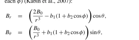
eachφ) (Kabin et al., 2007): Br =
2B 0
r3 −b1(1+b2cosφ)
cosθ, (14)
Bθ = B
0
r3 +b1(1+b2cosφ)
sinθ, (15)
Bφ = 0. (16)
So our approach based on axisymmetric geometry and wave Eq. (6) can only be approximately applied to the noon– midnight meridional planes corresponding toφ=0 andφ=
π, respectively, on which∂/∂φ=0.
Since the field remains planar (i.e.,Bφ=0), it is possible
to derive the field-line equation in each meridional plane (r, θ,φ≡Const) withrnormalized by the Earth radius:
dr dθ =
rBr
Bθ
=r(2/r
3−D)
1/r3+D cotθ, (17)
where we define a dimensionless quantity D≡ b1
B0(1+
b2cosφ). This leads to Hsin2θ= r
D·r3−2, (18) whereHis an integration constant. As usual, if we definer=
[image:4.612.308.547.428.498.2]-5 0 5
-5 0
5
X (R E)
Z (R
E
)
ˆ
n
ˆ
s
[image:5.612.83.253.67.181.2]⊗φˆ
Figure 2. The magnetic field lines of L=2,4,6 on the noon–
midnight meridional plane for the compressed dipole with B0=
0.31 Gauss,b1=10 nT andb2=8. The dashed lines mark the
lo-cations where the eigenfrequencies of the fundamental mode
inter-sect the critical frequencies, i.e., ω0=ωc as shown in Fig. 3 and
[image:5.612.308.548.95.272.2]given in Tables 2 and 3. The field-line-aligned orthogonal coordi-nate(n, s, φ)is also shown.
Table 2. List of parameters forL=2,4,6 of a compressed-dipole
field forφ=0 (noon).
L ω0, s−1 T0, s θ0,◦ r0(RE)
2 0.96 6.6 50 1.20
4 0.22 29 58 3.06
6 0.10 60 57 5.05
Then the colatitudeθF of one of the footpoints of one
partic-ularLshell is obtained by sin2θF =1/(H·D−2H ).
Subsequently, the necessary coefficients and factor in the KG Eq. (11) for the velocity perturbation in the toroidal mode are obtained as follows:
1 lu
= −1
lb
= 3
1+D·r3cotθ, (19)
1 Lu
= 7−4D·r
3−2D2r6
(1+D·r3)2 cotθ. (20) Additional coefficients such as 1/Mu can be derived from
Eq. (4) (Webb et al., 2012). Then Eq. (9) enables the deriva-tion of an analytic form of the critical frequencyωc
[image:5.612.88.249.317.372.2]appear-ing in the KG equation and the amplitude factorf (θ ), relat-ing the solution of the KG equation to the original physical perturbation quantity.
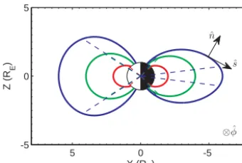
Figure 2 shows the selected field lines forL=2,4 and 6, respectively, in both the noon (φ=0) and midnight (φ=π) meridional planes of the Earth as illustrated. The asymmetry between the two sides is clearly seen due to the compression of the solar wind on the noon side (X>0). We carry out the analysis of toroidal-mode waves for each individual field line via the approach of KG equations outlined in Sect. 2.1.
First of all, the profiles of the critical frequency ωc and
the amplitude factor are calculated and illustrated in Fig. 3, together with the locations where the eigenfrequencies of the fundamental mode intersect the critical frequencies. The
Table 3. List of parameters forL=2,4,6 of a compressed-dipole
field forφ=π(midnight).
L ω0, s−1 T0, s θ0,◦ r0(RE)
2 0.94 6.7 48 1.11
4 0.18 34 45 1.86
6 0.060 105 83 (39) 5.81 (1.90)
0 10 20 30 40
1
√ F
π 4 π2 43π
10-2 10-1 100
ωc
(s
-1)
θ
0 10 20 30 40 50
1
√F
10-2 10-1 100
ωc
(s
-1)
θ
-1 -1
-1 -1 -1 π
4-1 π2-1 43π -1
(a) (b)
Figure 3. The parameter ωc (with B0=0.31 Gauss, a=6.4×
108cm andρe=7 amu cm−3) and the amplitude factor as a
func-tion ofθ for variousLvalues for the compressed-dipole field with
(a)φ=0 and (b)φ=π, respectively. Format is the same as Fig. 1.
The broken part of some curves corresponds toωc2<0.
corresponding parameters of the eigenfrequencyω0, the pe-riodT0, the colatitude θ0 and the radial distance r0 where ωc=ω0are given in Tables 2 and 3 for the noon and
mid-night side, respectively. The profiles ofωcandf show
signif-icant differences among the cases of noon, midnight merid-ional plane of the compressed dipole, and that of a standard dipole, especially for greaterLvalues. For example, for the caseL=6 on the midnight side, the amplitude factor peaks at a greater value (∼50) at the Equator, while the eigenfre-quencyω0 intersects the critical frequency at two locations inθ < π/2, one near the North Pole and the other near the Equator. Therefore, there are two separate regions of propa-gating solution to the KG equation whereω2> ω2c and one additional region of decaying solution surrounding the Equa-tor as marked by the pairs of dashed blue lines in Fig. 3b along congruent points in colatitude. However, for higher-order harmonics, the eigenfrequency increases with the in-creasing number of nodes such that it becomes greater than the critical frequency throughout the whole range of low lat-itudes enclosing the Equator.
[image:5.612.54.211.459.513.2]-0.5 0 0.5 bφ
θ
0 2 4
uφ
,E
n
×
40
π 4 2π 43π ω=0.1 s-1
-1 0 1 bφ
θ
0 1 2 3
uφ
,E
n
×
40
ω=0.06 s-1
-1 -1 -1 π 4-1 2π -1 43π -1
[image:6.612.48.287.67.173.2](a) (b)
Figure 4. Wave forms of the fundamental mode (L=6) on the
(a) noon and (b) midnight meridional plane (φ=0 andπ),
respec-tively. Dashed line denotes the electric field profile, with a multi-plication by 40. All units are arbitrary. The corresponding eigenfre-quency is denoted in the middle of each subplot.
seconds atL=6. The height (radial distances) of the loca-tions whereωc=ω0increase withLvalues, reaching much greater values in the compressed-dipole case than that in the standard dipole. The corresponding colatitudes, on the other hand, remain close to each other, except for the one near the Equator forL=6 on the midnight side of the compressed-dipole case.
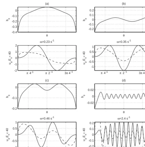
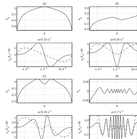
The choice ofL=6, which shows the greatest asymmetry between the noon side and midnight side of the compressed dipole, is a representative case to illustrate the spatial wave forms as harmonic solutions to the KG equation. The number of nodes, n, contained in the solution ofuφ increases from
0 in the fundamental mode to consecutive positive integral numbers for higher-order harmonics. Figure 4a, b show the fundamental modes for the noon and midnight side merid-ional planes of the compressed dipole. Similar to a standard-dipole case (Webb et al., 2012), thebφ profile contains one
node at the Equator, and the oscillating velocityuφand
elec-tric fieldEn, normal to the background field (see Fig. 2) are in phase, given the boundary conditionEn=0 at both foot-points. The fundamental-mode frequency on the midnight side is a little smaller than the noon side and the correspond-ingEnprofile has a significant dip (much reduced amplitude) near the Equator. These differences are caused by the differ-ent field-line geometry, the critical frequency and the ampli-tude factor for the two sides as discussed earlier. Such dif-ferences persist for higher-order harmonics. Figures 5 and 6 show the wave forms of higher-order harmonics of an in-creasing number of nodes on the noon and midnight side, respectively. The eigenfrequency increases with an increas-ing number of nodes. TheuφandEnperturbations remain in phase, while thebφoscillation is generally out of phase by
π/2. For the same harmonic mode, the midnight side solution always has a smaller eigenfrequency and a smaller amplitude inEnaround the Equator.
-0.4 -0.3 -0.2 -0.1 0
bφ
(a)
θ
-2 -1 0 1 2
uφ
,E
n
×
40
π 4 2π 3π 4
ω=0.23 s-1
-0.2 -0.1 0 0.1 0.2
bφ
(b)
θ
-1 -0.5 0 0.5 1
uφ
,E
n
×
40
ω=0.35 s-1
-0.2 -0.1 0
bφ
(c)
θ
-1 -0.5 0 0.5 1
uφ
,E
n
×
40
ω=0.46 s-1
-0.02 0 0.02
bφ
(d)
θ
-0.2 -0.1 0 0.1 0.2
uφ
,E
n
×
40
ω=2.4 s-1 -1 -1 -1 π 4-1 2π -1 3π 4-1
π 4-1 2π -1 3π 4-1 π 4-1 2π -1 3π 4-1
Figure 5. Harmonic wave forms (arbitrary unit) as derived from the
solutions of the KG equation on the noon meridional plane (φ=0)
of the compressed-dipole field for (a)n=1, (b)n=2, (c)n=3
and (d)n >4. Format is the same as Fig. 4 in each subplot.
3 Eigenvalue solutions of the poloidal mode
In the poloidal mode, both the magnetic field and velocity perturbations of the waves are in the meridional plane. The normal components perpendicular to the field line (see Fig. 2) are denotedbnandun, respectively. Therefore, the only
os-cillating electric field is along theφˆ direction,Eφand after
multiplied by a scaling factor,φ=rsinθ Eφ, is governed by
(Cummings et al., 1969; Oliver et al., 1993; Lee and Taka-hashi, 2006)
∇2φ+2rsinθ∇φ· ∇
1
rsinθ
+ω
2
VA2φ
=0, (21)
again assuming a harmonic time variation with angular eigenfrequency, ω. The scaling factor rsinθ arises from the curvilinear coordinate system, which is different from a Cartesian geometry. In an equivalent cylindrical coordinate (R, φ, Z)(∂/∂φ=0), it is written
∂2φ
∂R2 − 1 R
∂φ
∂R + ∂2φ
∂Z2 + ω2 VA2φ
=0. (22)
In a Cartesian geometry, the differential operator in the above equation becomes a single Laplacian and φ≡Eφ
(e.g., Cummings et al., 1969). Here the Alfvén speedVA=
[image:6.612.309.549.68.310.2]a 2-D domain such as a meridional plane of the compressed-dipole field forφ=0 andπonly. We are seeking eigenmode solutions subject to boundary conditionφ≡0 in the present
study. Once the electric field perturbation is obtained, the magnetic field perturbations,br andbθ, lying in the
merid-ional plane, can be derived via Faraday’s law using the linear approximations.
Interestingly, the magnetic field perturbation normal to the field line,bn, can be derived along each individual field
line following the previous approach by the equation below which follows from the linearized Faraday’s law:
∂bn
∂t = − Bθ
r2Bsinθ dφ
dθ . (23)
Note that the total derivative d/dθ here is evaluated along each individual field line and takes the form of Eq. (5). For harmonic oscillations, if we assign a phase lag ofπ/2 tobn
relative toEφat initial time, the left-hand side of Eq. (23)
be-comesωebn, which allows the derivation of a real-valued
am-plitude profile ofbnbased on solutions to Eq. (21). Similarly,
the tangential component of the magnetic field perturbation is obtained by
∂bs ∂t =
1
rsinθ(∇φ· ˆn)=
1
rsinθ
−Br
rB ∂φ ∂θ + Bθ B ∂φ ∂r . (24) In general, the right-hand side of the above equation does not vanish, indicating a compressional fast mode solution. On the other hand, if it does vanish, i.e.,∂φ/∂n=0, a standing
Alfvén wave mode should result.
3.1 Poloidal standing transverse (Alfvén) mode
This is a special case corresponding tobs≡0, i.e.,∂φ/∂n=
0 from Eq. (24) above. This corresponds to a transverse, Alfvén mode of poloidal polarization of the magnetic field perturbation that propagates along individual field lines. Therefore, we can apply exactly the same approach of Sect. 2. The electric field perturbation φ still satisfies
Eq. (21). However, when applying the conditionbs=0 and
projecting the partial differential equation (PDE) along an individual field line defined by a relation betweenrandθ, a wave equation of the form similar to Eq. (6) is obtained:
∂2φ
∂t2 = V2
r2 "
d2φ
dθ2 − d dθln
B2
Bθ2g(θ )sinθ !
dφ
dθ #
. (25)
Here the wave speed parameterV2≡Bθ2/(µ0ρ)remains the same as before, and the functiong(θ )is determined from a given background magnetic field model along an individual field liner(θ )by
d
dθlng(θ )= Br2 Bθ2
∂ ∂r rB θ Br . (26)
For example, for a standard-dipole field, the functiong(θ )=
sin2θis obtained.
-0.4 -0.2 0 0.2 0.4 bφ (b) θ -1 0 1 uφ ,E n × 40
ω=0.24 s-1
-0.3 -0.2 -0.1 0 bφ (c) θ -1 -0.5 0 0.5 1 uφ ,E n × 40
ω=0.33 s-1 -0.6 -0.4 -0.2 0 bφ (a) θ -1 0 1 uφ ,E n × 40
ω=0.15 s-1
-0.05 0 0.05 bφ (d) θ -0.2 0 0.2 uφ ,E n × 40
ω=1.7 s-1
π 4-1 2π -1 3π 4-1 π
4-1 2π -1 3π 4-1
π 4-1 2π -1 3π 4-1 π
[image:7.612.309.549.68.310.2]4-1 2π -1 3π 4-1
Figure 6. Harmonic wave forms on the midnight meridional plane
(φ=π) of the compressed-dipole field. Format is the same as
Fig. 5.
Therefore, the wave Eq. (25) can also be cast as a KG form and solved for eigenvalue solutions subject to the bound-ary conditionφ=0 at the footpoints of an individual field
line. In turn the magnetic field perturbation can be derived from Eq. (23). Below, we list the essential parameters for this mode conforming to the general descriptions in Sect. 2.1:
1 L
= d
dθln B2
Bθ2g(θ )sinθ !
, (27)
1 M
= 0 (28)
and the amplitude factor
f (θ )= B
Bθ p
g(θ )sinθ . (29) For the dipole field, the following explicit formulas are ob-tained
f (θ )=psinθ (1+3cos2θ ), (30)
1 L
=cotθ− 3 sin 2θ
1+3cos2θ. (31)
Thus, the critical frequency ωc can be written based on
10-2 10-1 100
ω c
(s
-1 )
θ
0 0.5 1 1.5
1
√ F
π 4-1 π2-1 43π -1
-1
Figure 7. The parameters ωc andf (θ )for the poloidal standing
Alfvén waves of the dipole field. Format is the same as Fig. 1.
Similarly, the critical frequency decreases from the poles to-ward the Equator where ωc2 becomes negative. The eigen-frequency of the fundamental mode generally intersects the critical frequency at mid- to low latitudes. The solution of the KG equation would also be a combination of a propagation type near the Equator and a decaying type near the two ends. The amplitude factor f (θ ), on the other hand, shows much less variation in magnitude and does not depend onL. Fig-ure 8 shows the fundamental-mode solutions forL=5, typi-cal of a standing wave with zero nodes in electric field pertur-bation. The amplitude ofEφdips slightly around the
Equa-tor. The eigenfrequency is 0.092 s−1, which corresponds to a period of 68 s. It compares well with observations to be dis-cussed below. Table 4 lists the corresponding parameters for the selectedLshells in the same format as Tables 1–3. The periods are in the same range as those of the toroidal mode.
For a compressed-dipole field, because the relation below r andθ along a field line is implicit, the relevant quanti-ties have to be evaluated numerically, especially the function g(θ )according to Eq. (26). In what follows, we provide solu-tions to the KG equation for the poloidal transverse mode in a compressed-dipole field with the magnetic field components given by Eqs. (14) to (16).
In this case, Eq. (26) becomes d
dθlng(θ )=
2+10Dr3−D2r6
(1+Dr3)2 cotθ=h(θ ), (32) where the radial distance r implicitly depends onθ as in-dicated by Eq. (18) along an individual field line. Therefore, the functiong(θ )has to be obtained by numerical integration ofh(θ ). Subsequently the coefficient functions 1/L and its
derivative with respect to θ appearing in the KG equation can be efficiently and accurately estimated by numerical dif-ferentiations.
The variations in the critical frequencyωc along
[image:8.612.85.252.65.231.2]individ-ual field lines ofL=2,4,6 for both the noon and midnight
Table 4. List of parameters forL=2,4,6 of a dipole field for
poloidal standing Alfvén waves.
L ω0, s−1 T0, s θ0,◦ r0(RE)
2 0.76 8.2 57 1.41
4 0.15 42 62 3.09
6 0.062 101 62 4.71
-10 0 10
b n
θ
0 0.1 0.2
E φ
ω=0.092 s-1
[image:8.612.342.511.97.333.2]π 4-1 π2-1 43π -1
Figure 8. Wave forms (arbitrary unit) of the fundamental mode
(L=5) for the poloidal standing Alfvén mode of the dipole field.
Format is the same as Fig. 4.
sides are shown in Fig. 9, together with the amplitude fac-torf (θ ). Compared with the corresponding variations of the dipole case in Fig. 7, the critical frequency again exhibits gaps whereω2c<0, but the profiles of the amplitude factor become dependent onL, for both sides. Then the KG equa-tion is solved for L=5 (M=0) and the solutions
corre-sponding to the fundamental mode are given in Fig. 10. They exhibit very similar behavior to the solution of the dipole field given in Fig. 8 except that the corresponding eigenfre-quencies are different such that the one for the dipole field is in-between the ones for the compressed-dipole cases. The corresponding periods of the compressed-dipole cases are 52 s and 93 s, respectively, for the noon and midnight side. It is worth noting that for these poloidal modes of different background field configurations, gaps always exist in the crit-ical frequencies whereω2c<0. Therefore, the propagating-type solutions corresponding toω2> ω2calways exist in this mode. In other words, there is no lower bound in these cases on the wave frequency.
3.2 A real-case study of poloidal standing Alfvén mode
In this subsection, we demonstrate the validity of our ap-proach by comparing our analysis result with a recent direct spacecraft observation of poloidal standing Alfvén waves by Dai et al. (2013). Since these observations occurred near
magne-10-2
10-1
100
ωc
(s
-1)
θ
1 2 3 4
1
√
F
10-2
10-1
100
ωc
(s
-1)
θ
1 2 3 4
1
√
F
(a) (b)
-1 -1
π 4-1 π2 4-1 3π -1
[image:9.612.50.290.67.190.2]π 4-1 π2 4-1 3π -1
Figure 9. The parameterωcand the adiabatic growth and decay
fac-tor as a function ofθfor variousLvalues of the poloidal transverse
mode for the compressed-dipole field with (a)φ=0 and (b)φ=π,
respectively. Format is the same as Fig. 1. The broken part of some
curves in top panels corresponds toω2c<0.
tosphere, we present the analysis results of the dipole and the compressed-dipole field, which offer different background field geometries. Figure 11 shows our results of suitable physical units forL=5 with the same set of parameters as Dai et al. (2013), ρe=6.4 amu cm−3 and the power index
1.0 of the density variation, to facilitate a direct compari-son with their results (Fig. 3 therein). Dai et al. (2013) used a theoretical model of Cummings et al. (1969) and realistic ionosphere boundary conditions of finite conductivity at the footpoints of the field line. Therefore, their solutions ofEφ
and bn profiles are of non-zero values at the ends and are
asymmetric about the Equator, whereas ours are symmetric andEφvanishes at the two ends. Nonetheless the spatial
pro-files over the mid- to low latitudes still compare very well. In both columns, the magnitudes of both perturbations show a slight decrease toward the Equator in Eφ and a rapid
in-crease toward the ends inbn. In particular, the wave periods
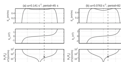
of the two cases are 45 s and 82 s, while the observed value is 84 s, closer to the period of the midnight side. The ratios of
|bn/Eφ|at the spacecraft location (∼17◦south in latitude)
are 0.15 and 0.30 nT/(mV/m) from Fig. 11a and b, respec-tively, while the observed value is 0.3 nT/(mV/m), identical to the latter of the ratios. Our result is also consistent with the observation in thatEφ leads the phase ofbn byπ/2 as
discussed earlier. The corresponding wave period and ampli-tude ratio of the fundamental poloidal mode for the standard-dipole field by using the above set of parameters are 60s and 0.21 nT/(mV/m), given in Fig. 12, respectively, values which are somewhere in between those values presented for the two sides of the compressed dipole. The estimates of these quan-tities in Dai et al. (2013) by a different theoretical model are 62 s and 0.25 nT/(mV/m), respectively. Thus, this particular ULF wave observation is consistent with our model results.
-20 0 20
bn
θ
0 0.2 0.4 Eφ
ω=0.121 s-1
-20 0 20
bn
θ
0 0.2 0.4
Eφ
ω=0.0678 s-1
(a) (b)
[image:9.612.307.549.67.180.2]π 4-1 π2-1 43π -1 π 4-1 π2-1 43π -1
Figure 10. Wave forms of the poloidal fundamental mode (L=5)
on the (a) noon(φ=0) and (b) midnight (φ=π) meridional plane,
respectively. Format is the same as Fig. 8.
-1 0 1
bn
(nT)
0 0.2 0.4
Eφ
(mV/m)
(a) ω=0.141 s-1, period=45 s
10-2 10-1 100 101
|bn /Eφ
|
(nT)/(mV/m)
-2 0 2
bn
(nT)
0 0.2 0.4
Eφ
(mV/m)
(b) ω=0.0763 s , period=82 s-1
10-2 10-1 100 101
θ
|bn /Eφ
|
(nT)/(mV/m)
π 4-1 π2-1 3π4-1
θ
π 4-1 π2-1 3π4-1
Figure 11. The solutions ofEφ(in mV/m),bn(in nT) and the ratio
inbetween (from top to bottom panels) for the compressed dipole on the (a) noon side and (b) midnight side, to be compared with the spacecraft observations of Dai et al. (2013). The vertical dashed line denotes the spacecraft location and the cross marks the measured
ratio (∼0.3 nT/(mV/m)) during the time period of measurements.
3.3 Poloidal compressional mode
In the case thatbs6=0, Eq. (22) has to be solved in a 2-D
domain as an eigenvalue problem subject to the boundary condition Eφ=0 on all sides. We have solved the
equa-tion and obtained the corresponding eigenmode soluequa-tions of a discrete set of increasing eigenfrequencies by utilizing the software package PDE2D.1The solutions are also cross-checked with the Matlab PDE toolbox and identical results are obtained. The computational domain is chosen as r∈ [1, Lp]RE andθ∈ [θp, π−θp], where θp=arcsinp1/Lp.
We choose Lp=7 in order to avoid the singular point in
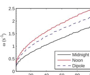
the compressed-dipole field model as well as the singular-ity along the poles (X=0). We apply the dipole field and the compressed-dipole field models and the same density distri-bution as before for the background field and plasma condi-tions. Three sets of eigenfrequencies of ascending order of magnitude (mode) are obtained for both the noon and mid-night side meridional planes of the compressed-dipole field and the standard-dipole field. The first 100 eigenfrequencies
[image:9.612.310.549.242.363.2]-0.5 0 0.5
bn
(nT)
0 0.1 0.2
Eφ
(mV/m)
ω=0.105 s , period=60 s-1
10-2 10-1 100 101
θ |bn
/Eφ
|
(nT)/(mV/m)
[image:10.612.88.250.70.245.2]π 4-1 π2-1 3π4-1
Figure 12. The solutions ofEφ(in mV/m),bn(in nT) and the ratio
inbetween (from top to bottom panels) for the standard dipole of the same set of parameters as Dai et al. (2013). Format is the same as Fig. 11.
20 40 60 80 100
0 0.5 1 1.5 2 2.5
Mode
ω
(s
-1 )
Midnight Noon Dipole
Figure 13. The first 100 eigenfrequencies for the noon side and midnight side of the compressed dipole and a standard-dipole field.
are shown in Fig. 13. They generally exhibit a rapid rise at the lowest numbers of mode; then the trend of increase seems to become more gradual and eventually linear. At one specific mode, the eigenfrequency of the noon side is always greater than that of the midnight side, while the value of the dipole case is always inbetween, albeit slightly closer to the value of the noon side. The corresponding eigenmode solutions (not shown) generally display a regular pattern of nodal structures of progressively increasing number of nodes with increasing eigenfrequencies. Our preliminary numerical experiments in-dicate that the background magnetic field greatly affects the eigenvalue solutions.
4 Conclusions and discussion
In conclusion, we have examined, in a fairly comprehen-sive manner, the decoupled toroidal and poloidal-mode hy-dromagnetic waves in cold plasmas with applications to
the Earth’s inner magnetosphere (ULF waves), represented by a compressed-dipole field model in addition to the standard-dipole field. Under certain assumptions, the decou-pled wave equations are recast as the Klein–Gordon (KG) form along individual magnetic field lines, especially for both the toroidal and poloidal transverse Alfvén waves. Such a KG equation describes the effect of background medium on wave propagation (Morse and Feshbach, 1953), as embodied in the term involving the critical frequency,ωc. We obtain the
spatial profiles of the characteristic parameters in the KG for-mulations including the critical frequencyωcand the
ampli-tude factorf, both as functions of the colatitude,θ. The for-mer generally exhibits a behavior of minimum values below 0.1 Hz (sometimes 0.01 Hz) near the Equator and increasing values towards the footpoints, exceeding 1 Hz. This leads to a spatially composite solution of a propagating type where the eigenfrequencyω > ωcusually occurs near the Equator
and a decaying type whereω < ωc occurs toward the
foot-points. The latter modulates the amplitude of the wave forms spatially. We obtain the sets of eigenvalue solutions of in-creasing eigenfrequencies and the number of nodes in the wave forms for different background magnetic field geome-tries. The corresponding wave periods are on the order of∼1 to∼100 s and compare well quantitatively with prior stud-ies and observations. In particular, we present a case study of a fundamental poloidal Alfvén wave via our approach and compare our results with a direct spacecraft observation by Dai et al. (2013). The observed wave period∼84 s and the amplitude ratio∼0.3 nT/(mV/m) agree with our ranges of estimates – 45–82 s and 0.15–0.3 nT/(mV/m), respectively. Thus, we provide a relatively simple yet reliable means of analyzing ULF wave observations in the magnetosphere.
The main intellectual merits of this work lie in the aspect of the unique approach via the KG equations for both the toroidal and poloidal transverse Alfvén waves for a given background magnetic field geometry. The existence of the critical frequency indicates the importance of the background magnetic field topology. For some instances, a propagating wave mode can only exist above a certain frequency, i.e., the minimumωc. In particular, the case study of a direct
[image:10.612.92.241.317.441.2]to extend the applications to the solar coronal loop oscilla-tions as we did in Hu et al. (2012).
Acknowledgements. We dedicate this paper to the late James F. McKenzie, who initiated this work during his visit and was partially supported by the Pei-Ling Chan Chair of Physics of the University of Alabama in Huntsville and the NRF of South Africa. His infectious enthusiasm for the subject motivated us to complete this work in his honor. He will be missed as a colleague, a mentor and a friend. The other authors acknowledge partial support of NSF grant AGS-1062050 and NASA grant NNX12AH50G. J. Zheng especially acknowledges partial support of a graduate research assistantship through the NASA grant. We are also grateful to G. Sewell for his help with the PDE2D software package. Q. Hu acknowledges useful discussions with C.-S. Wu, Bo Li, Yao Chen and Lidong Xia and is grateful for their hospitality during his visit to Shandong University, Weihai, China. We also thank the reviewers for their constructive comments.
The topical editor, G. Balasis, thanks the three anonymous referees for help in evaluating this paper.
References
Chen, L. and Cowley, S. C.: On field line resonances of hydromag-netic Alfven waves in dipole maghydromag-netic field, Geophys. Res. Lett., 16, 895–897, doi:10.1029/GL016i008p00895, 1989.
Claudepierre, S. G., Hudson, M. K., Lotko, W., Lyon, J. G., and Denton, R. E.: Solar wind driving of magnetospheric ULF waves: Field line resonances driven by dynamic pres-sure fluctuations, J. Geophys. Res.-Space, 115, A11202, doi:10.1029/2010JA015399, 2010.
Cummings, W. D., O’Sullivan, R. J., and Coleman, Jr., P. J.: Stand-ing Alfvén waves in the magnetosphere, J. Geophys. Res., 74, 778, doi:10.1029/JA074i003p00778, 1969.
Dai, L., Takahashi, K., Wygant, J. R., Chen, L., Bonnell, J., Cat-tell, C. A., Thaller, S., Kletzing, C., Smith, C. W., MacDowall, R. J., Baker, D. N., Blake, J. B., Fennell, J., Claudepierre, S., Funsten, H. O., Reeves, G. D., and Spence, H. E.: Excita-tion of poloidal standing Alfvén waves through drift resonance wave-particle interaction, Geophys. Res. Lett., 40, 4127–4132, doi:10.1002/grl.50800, 2013.
Dai, L., Takahashi, K., Lysak, R., Wang, C., Wygant, J. R., Kletzing, C., Bonnell, J., Cattell, C. A., Smith, C. W., Mac-Dowall, R. J., Thaller, S., Breneman, A., Tang, X., Tao, X., and Chen, L.: Storm time occurrence and spatial distribution of Pc4 poloidal ULF waves in the inner magnetosphere: A Van Allen Probes statistical study, J. Geophys. Res.-Space, 120, 4748– 4762, doi:10.1002/2015JA021134, 2015.
Degeling, A. W., Rankin, R., Kabin, K., Rae, I. J., and Fenrich, F. R.: Modeling ULF waves in a compressed dipole magnetic field, J. Geophys. Res.-Space, 115, A10212, doi:10.1029/2010JA015410, 2010.
Dimitrakoudis, S., Mann, I. R., Balasis, G., Papadimitriou, C., Anastasiadis, A., and Daglis, I. A.: Accurately specifying storm-time ULF wave radial diffusion in the radiation belts, Geophys. Res. Lett., 42, 5711–5718, doi:10.1002/2015GL064707, 2015.
Dungey, J. W.: Electrodynamics of the Outer Atmosphere, in: Physics of the Ionosphere, London, The Physical Society, 229 pp., 1955.
Dungey, J. W.: Hydromagnetic waves and the ionosphere, in: The Ionosphere, London: The Institute of Physics and the Physical Society, edited by: Stickland, A. C., 230 pp., 1963.
Elkington, S. R.: A Review of ULF Interactions With Radiation Belt Electrons, in: Magnetospheric ULF Waves: Synthesis and New Directions, edited by: Takahashi, K., Chi, P. J., Denton, R. E., and Lysak, R. L., 169 , Washington DC American Geophysical Union Geophysical Monograph Series, 177 pp., 2006.
Elkington, S. R., Hudson, M. K., and Chan, A. A.: Acceleration of relativistic electrons via drift-resonant interaction with toroidal-mode Pc-5 ULF oscillations, Geophys. Res. Lett., 26, 3273– 3276, doi:10.1029/1999GL003659, 1999.
Elkington, S. R., Hudson, M. K., and Chan, A. A.: Resonant ac-celeration and diffusion of outer zone electrons in an asym-metric geomagnetic field, J. Geophys. Res.-Space, 108, 1116, doi:10.1029/2001JA009202, 2003.
Fraser, B. J.: ULF Waves-A Historical Note, in: Magnetospheric ULF Waves: Synthesis and New Directions, edited by: Taka-hashi, K., Chi, P. J., Denton, R. E., and Lysak, R. L., 169, Wash-ington DC American Geophysical Union Geophysical Mono-graph Series, p. 5, 2006.
Hu, Q., McKenzie, J. F., and Webb, G. M.: Klein-Gordon equa-tions for horizontal transverse oscillaequa-tions in two-dimensional coronal loops, Astron. Astrophys., 541, A53, doi:10.1051/0004-6361/201117421, 2012.
Kabin, K., Rankin, R., Mann, I. R., Degeling, A. W., and Marchand, R.: Polarization properties of standing shear Alfvén waves in non-axisymmetric background magnetic fields, Ann. Geophys., 25, 815–822, doi:10.5194/angeo-25-815-2007, 2007.
Kivelson, M. G.: ULF waves from the ionosphere to the outer plan-ets, in: Magnetospheric ULF Waves: Synthesis and New Direc-tions, edited by: Takahashi, K., Chi, P. J., Denton, R. E., and Lysak, R. L., 169, Washington DC American Geophysical Union Geophysical Monograph Series, 11–30, doi:10.1029/169GM04, 2006.
Lee, D.-H. and Takahashi, K.: MHD Eigenmodes in the Inner Mag-netosphere, in: Magnetospheric ULF Waves: Synthesis and New Directions, edited by: Takahashi, K., Chi, P. J., Denton, R. E., and Lysak, R. L., 169, Washington DC American Geophysical Union Geophysical Monograph Series, p. 73, 2006.
Liu, W., Sarris, T. E., Li, X., Zong, Q.-G., Ergun, R., Angelopoulos, V., and Glassmeier, K. H.: Spatial structure and temporal evolu-tion of a dayside poloidal ULF wave event, Geophys. Res. Lett., 38, L19104, doi:10.1029/2011GL049476, 2011.
Liu, W., Cao, J. B., Li, X., Sarris, T. E., Zong, Q.-G., Hartinger, M., Takahashi, K., Zhang, H., Shi, Q. Q., and Angelopou-los, V.: Poloidal ULF wave observed in the plasmasphere boundary layer, J. Geophys. Res.-Space, 118, 4298–4307, doi:10.1002/jgra.50427, 2013.
McKenzie, J. F. and Hu, Q.: Klein-Gordon equations for toroidal hydromagnetic waves in an axi-symmetric field, Ann. Geophys., 28, 737–742, doi:10.5194/angeo-28-737-2010, 2010.
Oliver, R., Ballester, J. L., Hood, A. W., and Priest, E. R.: Mag-netohydrodynamic waves in a potential coronal arcade, Astron. Astrophys., 273, 647–658, 1993.
Singer, H. J., Southwood, D. J., Walker, R. J., and Kivelson, M. G.: Alfven wave resonances in a realistic magnetospheric magnetic field geometry, J. Geophys. Res., 86, 4589–4596, doi:10.1029/JA086iA06p04589, 1981.
Southwood, D. J. and Hughes, W. J.: Theory of hydromagnetic waves in the magnetosphere, Space Sci. Rev., 35, 301–366, doi:10.1007/BF00169231, 1983.
Takahashi, K., Denton, R. E., and Gallagher, D.: Toroidal wave frequency at L = 6-10: Active Magnetospheric Par-ticle Tracer Explorers/CCE observations and comparison with theoretical model, J. Geophys. Res.-Space, 107, 1020, doi:10.1029/2001JA000197, 2002.
Takahashi, K., Hartinger, M. D., Angelopoulos, V., Glassmeier, K.-H., and Singer, H. J.: Multispacecraft observations of funda-mental poloidal waves without ground magnetic signatures, J. Geophys. Res.-Space, 118, 4319–4334, doi:10.1002/jgra.50405, 2013.
Tamao, T.: Transmission and coupling resonance of hydromag-netic disturbances in the non-uniform Earth’s magnetosphere, Sci. Rep. Tohoku Univ., Ser. 5, Geophys., 17, 43–72, 1965. Ukhorskiy, A. Y., Takahashi, K., Anderson, B. J., and
Ko-rth, H.: Impact of toroidal ULF waves on the outer radi-ation belt electrons, J. Geophys Res.-Space, 110, A10202, doi:10.1029/2005JA011017, 2005.
Volwerk, M.: Multi-Satellite Observations of ULF Waves, in: Mag-netospheric ULF Waves: Synthesis and New Directions, edited by Takahashi, K., Chi, P. J., Denton, R. E., and Lysak, R. L., vol. 169, Washington DC American Geophysical Union Geophysical Monograph Series, p. 109, 2006.