https://doi.org/10.5194/bg-14-4161-2017 © Author(s) 2017. This work is distributed under the Creative Commons Attribution 3.0 License.
Process-based modelling of NH
3
exchange with grazed grasslands
Andrea Móring1,2,3, Massimo Vieno2, Ruth M. Doherty3, Celia Milford4,5, Eiko Nemitz2, Marsailidh M. Twigg2, László Horváth6, and Mark A. Sutton2
1University of Edinburgh, High School Yards, Edinburgh, EH8 9XP, UK 2Centre for Ecology and Hydrology, Bush Estate, Penicuik, EH26 0QB, UK
3University of Edinburgh, The King’s Buildings, Alexander Crum Brown Road, Edinburgh, EH9 3FF, UK
4Associate Unit CSIC University of Huelva ”Atmospheric Pollution”, CIQSO, University of Huelva, Huelva, E21071, Spain 5Izaña Atmospheric Research Centre, AEMET, Joint Research Unit to CSIC “Studies on Atmospheric Pollution”,
Santa Cruz de Tenerife, Spain
6Hungarian Meteorological Service, Gilice tér 39, Budapest, 1181, Hungary Correspondence to:Mark A. Sutton ([email protected])
Received: 22 December 2016 – Discussion started: 16 January 2017
Revised: 22 June 2017 – Accepted: 14 July 2017 – Published: 21 September 2017
Abstract. In this study the GAG model, a process-based ammonia (NH3) emission model for urine patches, was extended and applied for the field scale. The new model (GAG_field) was tested over two modelling periods, for which micrometeorological NH3 flux data were avail-able. Acknowledging uncertainties in the measurements, the model was able to simulate the main features of the ob-served fluxes. The temporal evolution of the simulated NH3 exchange flux was found to be dominated by NH3 emis-sion from the urine patches, offset by simultaneous NH3 deposition to areas of the field not affected by urine. The simulations show how NH3 fluxes over a grazed field in a given day can be affected by urine patches deposited several days earlier, linked to the interaction of volatilization pro-cesses with soil pH dynamics. Sensitivity analysis showed that GAG_field was more sensitive to soil buffering capacity (β), field capacity (θfc)and permanent wilting point (θpwp) than the patch-scale model. The reason for these different sensitivities is dual. Firstly, the difference originates from the different scales. Secondly, the difference can be explained by the different initial soil pH and physical properties, which determine the maximum volume of urine that can be stored in the NH3 source layer. It was found that in the case of urine patches with a higher initial soil pH and higher initial soil water content, the sensitivity of NH3exchange toβ was stronger. Also, in the case of a higher initial soil water con-tent, NH3exchange was more sensitive to the changes inθfc andθpwp. The sensitivity analysis showed that the nitrogen
content of urine (cN)is associated with high uncertainty in the simulated fluxes. However, model experiments based on cN values randomized from an estimated statistical distribu-tion indicated that this uncertainty is considerably smaller in practice.
Finally, GAG_field was tested with a constant soil pH of 7.5. The variation of NH3 fluxes simulated in this way showed a good agreement with those from the simulations with the original approach, accounting for a dynamically changing soil pH. These results suggest a way for model sim-plification when GAG_field is applied later at regional scale.
1 Introduction
change? A way to address this question and predict the en-vironmental consequences is to design meteorology-driven NH3 emission models for each agricultural source (Sutton et al., 2013). This study represents a step toward this goal by describing an NH3exchange model for grazed fields, ac-counting for the relevant meteorological drivers.
As confirmed by both laboratory and field studies (Far-quhar et al., 1980; Sutton et al., 1995), the exchange of NH3 between surface and atmosphere is bidirectional. The direc-tion of the net NH3exchange is controlled by the difference in the relative magnitude of atmospheric NH3concentration at two heights above the surface: the so-called “compen-sation point” (atmospheric NH3 concentration right above the surface) and the ambient atmospheric NH3 concentra-tion (high above the surface). If the compensaconcentra-tion point is the larger of the two, NH3is emitted to the atmosphere, whilst if the ambient air concentration is the larger, net deposition takes place, transferring NH3 to the surface. The state-of-the-art modelling technique for this bidirectional behaviour is the application of a “canopy compensation point” model (Sutton et al., 1995; Nemitz et al., 2001; Burkhardt et al., 2009; Flechard et al., 2013). These models derive the net NH3emission flux over a canopy by taking into account the NH3exchange with the different sources and sinks within the canopy (e.g. stomata, leaf surface, soil, litter) as well as the effect of meteorological variables and the canopy on these component NH3fluxes.
Over a grazed field the dominant source of NH3is urine rather than dung (Petersen et al., 1998; Laubach et al., 2013). Therefore, the NH3 exchange over a grazed field is deter-mined by two main components: the NH3emission from the urine patches and the NH3 exchange with the area on the field that is not affected by urine (“non-urine area”). The GAG model (Generation of Ammonia from Grazing; Móring et al., 2016) is a special application of a canopy compensa-tion point model that derives NH3volatilization from a unit of NH3source on a grazed field: a single urine patch. GAG calculates NH3 emission from a urine patch in a process-based way, simulating the total ammoniacal nitrogen (TAN) and water content under the urine patch as well as the evo-lution of soil pH. The present paper describes an extension of the GAG model, so that it accounts for the NH3emission from all of the urine patches deposited over a time interval on a grazed field and the NH3exchange with the non-urine area.
The primary goal of this model development was to con-struct a tool that can be used in further studies to gain insights on the effects of meteorological variables on NH3emission from grazing. Furthermore, our aim was to design a model that can be applied to an atmospheric chemistry transport model. Such a model application would serve as a base for future research, investigating how altered climate can affect NH3emission, dispersion and deposition on a larger scale – i.e. regional or global scale. Therefore, simplicity was a key aspect in the model development presented here, while
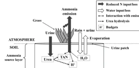
tak-Figure 1.Simplified schematic of the GAG model by Móring et al. (2016), referred to as GAG_patch in this study.
ing into account physical and chemical processes that can be relevant over these larger scales.
In the following, firstly, the theoretical background of the field-scale model application is presented (Sect. 2). Secondly, the equations required for upscaling to a field are provided, as well as the data used in the model evaluation and the meth-ods applied in the sensitivity analysis (Sect. 3). This is fol-lowed by presentation of the model simulations for two ex-perimental periods and the outcomes of the sensitivity analy-sis (Sect. 4). Finally, we conclude the paper with a discussion of the results and our conclusions (Sects. 5 and 6).
2 Theoretical background
2.1 Description of the GAG model
The GAG model, applied and extended to the field scale in this study, is a process-based NH3 emission model for a single urine patch. An in-depth description of the model, together with a comprehensive sensitivity analysis can be found in Móring et al. (2016) and Móring (2016). The GAG model is capable of simulating the driving soil chemistry by accounting for the TAN and the water content of the soil un-der the urine patch (in Fig. 1, TAN budget and water budget, respectively) and the variation of soil pH (H+ion budget in Fig. 1). Following the considerations of Móring et al. (2016), the model handles urine as a water solution of urea, i.e. the urinary N content is assumed to be in the form of urea. The TAN and the H+ion budgets are controlled by the hydrolysis of the urea content of urine, as well as the NH3emission from the soil. In the water budget, apart from the liquid content of the incoming urine, precipitation acts as a source term, whilst soil evaporation is considered as the only sink term.
[image:2.612.309.551.69.187.2]capil-Figure 2.Difference in the chemical composition of the soil in two urine patches deposited at different times. The different colours of the old and the newly deposited urine patches (black and white, respectively) as well as the overlap between them (grey) show the different soil chemical properties in the different areas.
lary rise) as well as the mixing of urea and the products of its hydrolysis within the solution was neglected. Hereafter, the original GAG model for patch scale and its extended version for field scale are referred to as GAG_patch and GAG_field, respectively.
2.2 Assumptions for the model application at field scale
Among all the naturally varying factors related to urination events during grazing, the following sections describe those that are likely to be the most relevant from the point of view of NH3 exchange over a grazed field. Firstly, the possible overlap of the patches is examined (Sect. 2.2.1), then fur-ther parameters are discussed that can vary among urination events, such as the area of the patches (Apatch), the frequency of urination events (UF) and the nitrogen content of urine (cN; Sect. 2.2.2). Finally, model assumptions for calculating the total NH3net flux for the field are identified (Sect. 2.2.3).
2.2.1 Exclusion of the overlap of the urine patches
According to observations (e.g. Betteridge et al., 2010; Moir et al., 2011; Dennis et al., 2013), urine patches over a grazed paddock may overlap. It was found that the overlap can have a large effect on N leaching (Pleasants et al., 2007; Shorten and Pleasants, 2007); however, no studies are available that investigate the effect of overlap in particular on NH3 emis-sion from urine patches.
It is reasonable to assume that the emission flux from the area of the overlap will differ from both the previously and the newly deposited patches due to the differences in the soil chemical properties (Fig. 2). Since urea hydrolysis is in a dif-ferent stage in the two urine patches, the soil chemistry under them will be different, and their mixture under the overlap is likely to result in a third, different chemical composition. In addition, if patches partly cover each other, the total source area will be smaller than if they were completely separate, which may influence the total NH3emission from the field. Therefore, it is likely that the possible overlap of the patches affects NH3emission. However, to predict in every time step of the model which patches will cover each other, and what size the overlap will be, is very difficult. Thus, it would be preferable to neglect the overlap of the patches if the error
from this simplification can be shown to be small. To assess the resulting error arising from such a simplification, the dif-ference in the field proportion covered by urine patches was investigated between the two cases: when overlap is assumed and when it is excluded.
A way to estimate the temporal evolution of the urine-covered proportion of the field is to use a negative binomial distribution function for the time–space distribution of the urine patches as suggested by Petersen et al. (1956), or the Poisson distribution tested by Romera et al. (2012). Based on the distribution suggested by Petersen et al. (1956), Pakrou and Dillon (2004) determined the proportion of the paddock covered by urine patches (Pt)after attime period as
Pt=1−q−K, (1)
whereKis a parameter that represents the uniformity of the excretal distribution. Following Pakrou and Dillon (2004), a representative value ofK=7 was used. The value of q is calculated as
q=Dt+K
K , (2)
in whichDt is the proportion of the urine-covered area over
at time period if there is no overlap (Eq. 3), i.e. the total number of the patches (Nt)deposited overt multiplied by Apatchand divided by the field area (Afield):
Dt=
NtApatch Afield
. (3)
UsingDt, Romera et al. (2012) derivedPt assuming a
Pois-son distribution as follows:
Pt=1−e−Dt, (4)
whereeis Euler’s constant (∼2.718).
To investigate the highest possible difference that the ex-clusion of overlap can cause, in the following calculation a “worst case scenario” was assumed with the highest possible coverage by urine, i.e. the highest realistic animal density over a field, the largestApatchand the highest UF. The ranges of all these parameters are listed in Table 1 for sheep and cattle, together with their references.
According to the agricultural statistics of the European Commission for 2010 (EC, 2015), the maximal grazing animal densities on the agricultural holdings Europe-wide were higher than 10 LSU ha−1(where LSU stands for live-stock unit, which equals to 1 dairy cow or 10 sheep). Since no higher values than 10 were identified, 10 LSU ha−1 was assumed as the maximum. The value of Nt was
cal-culated as the product of animal density over a hectare (Afield=10 000 m2)and the maximum daily UF (urination events per animal per day, Table 1).
Figure 3 shows Pt, using the two different equations,
[image:3.612.50.286.65.125.2]Table 1.Ranges of the parameters used in the calculation of the urine-covered proportion of a field with an area of 1 ha (=10 000 m2).
Animal Sheep Cattle Reference
Number of animals onAfield 1–100 0.1–10 EC (2015)
Urination frequency (UF) 15–20 8–12 Whitehead (1995)
(urination animal−1day−1)
Patches deposited per day (Nt) 15–2000 0.8–120 –
Patch area (Apatch; m2) 0.043–0.055 0.38–0.42 Williams and Haynes (1994)
Figure 3.Proportion of the field covered by urine patches (Pt) cal-culated for sheep(a)and cattle(b)as suggested by Pakrou and Dil-lon (2004;Pt_Pakrou), Romera et al. (2012;Pt_Romera)and when
there is no overlap between the patches (Dt).
with slightly smaller values from Eq. (1). Therefore, for further investigation the Pt values from Pakrou and
Dil-lon (2004; Eq. 1) were taken and compared with the no-overlap case (Pt=Dt). In the case of sheep (Fig. 3a), the
difference betweenPt andDt became higher than 5 % after
the eighth day (and exceeds 10 % after the 16th day – not
shown here), whilst in the case of cattle (Fig. 3b) the same occurred after the 17th day.
The great majority of NH3is emitted in the first 8 days af-ter the deposition of a urine patch (Sherlock and Goh, 1985). This means that after the eighth day the NH3exchange flux over the urine patches will be very close to that of the un-affected area of the field. Presumably (as suggested by the model results in Móring et al., 2016) at this stage the chemi-cal composition of the soil solution in the source layer under these patches will be also close to that of the initial, unaf-fected soil. Thus, practically, the patches deposited 8 or more days before the given time step can be treated as part of the unaffected area of the field, or in other words, these patches disappear from the field. As a consequence, the total area of the patches grows in the first 8 days, then it remains constant while the animals are on the field. Therefore, the probabil-ity of overlap after the eighth day will be the same as on the eighth day, since the total area of the patches prone to overlap with the new patches does not change after the eighth day.
Finally, it has to be noted that the results in Fig. 3 illus-trate an extreme situation (the “worst case scenario”), and in realityPt is much likely to grow rather more slowly. This
allows a longer time before the exceedance of the 5 % differ-ence inPt between the overlap and no-overlap case. Hence,
for field-scale application of GAG the effect of overlap be-tween the patches was concluded to be negligible, assuming completely separated urine patches in every time step.
[image:4.612.74.260.185.565.2]can therefore be generally neglected for continuous grazing and short periods of rotational grazing, we acknowledge that there may be some extreme cases of intense extended grazing where patch overlap could become relevant.
2.2.2 Assumptions forAptach, UF andcN
As shown in the previous section, the parameters that regu-late the extent of the field covered by urine are (i) the number of the animals on the field, (ii)Apatchand (iii) UF. The first parameter at a field-scale model application is easy to ob-tain, but the observations of the area of every single urine patch, as well as the number of urinations on an hourly ba-sis, are rather difficult (see the overview of the observation techniques in Dennis et al., 2013).
Therefore, for GAG_field, a constantApatchfor every in-dividual urination event and a constant UF were assumed. There are values reported forApatchin the literature (Table 1), whose average was used in the baseline simulations and with a sensitivity test an estimation was given for the uncertainty resulting from this simplification (Sect. 4.2.5).
In the literature observational data can be also found for UF (as shown in Table 1), but the temporal resolution of these data is usually a day. Based on personal communication with farmers, the hourly number of urine patches deposited over a field varies between the grazing and rumination periods and also between day and night. However, for the current mod-elling study an even distribution of urination events was as-sumed over the day, dividing the reported average daily UF by 24 h. As forApatch, a sensitivity analysis was carried out for this parameter as well (Sect. 4.2.5).
Another feature of the individual urination events that strongly influences the subsequent NH3volatilization iscN. This parameter ranges widely (2–20 g N dm−3; Whitehead, 1995), not just amongst different animals but also for differ-ent urination evdiffer-ents by the same animal (Betteridge et al., 1986; Hoogendoorn et al., 2010). In the baseline simulation a constant average N content was applied. In Sect. 4.2.5, the response of the model was analysed to this choice ofcNand also to the uncertainty originating from the temporal varia-tion of this parameter.
2.2.3 Assumptions for the calculation of the net NH3flux
[image:5.612.307.551.67.185.2]With all the above assumptions, two types of area can be dis-tinguished over a grazed field: (a) area covered by urine, and (b) area that is not affected by urine, referred to hereafter as “non-urine area” (as shown on Fig. 4). Therefore, it was as-sumed that the total flux over the field is the sum of the emis-sion from the urine-affected area and the exchange with the non-urine area. Over the urine-affected area the GAG model was applied to every single urine patch and for the non-urine area a modified version of the GAG model was used, as-suming constant emission potentials, as explained later, in
Figure 4.The schematic of GAG_field. The figure depicts the com-ponents of the total net NH3flux over the field: NH3emission from
the urine patches and the NH3exchange with the non-urine area.
Sect. 3.1. One of the challenges of simulating bidirectional exchange at the field scale is that fluxes are both driven by atmospheric concentrations (χa)– especially for deposition – and affect atmospheric concentrations – especially for emis-sion (e.g. Loubet et al., 2009). In addition, due to the urine patches, a grazed field is not a uniform source of NH3. One of the consequences is that the atmospheric concentration of NH3is not homogeneous over the field (see e.g. Bell et al., 2017). Both effects result in a horizontal advection of NH3, neglecting which leads to an error of the estimation of the to-tal NH3flux. At the field scale, this effect can be explored by explicit consideration of horizontal gradients (Loubet et al., 2009) or by sensitivity analysis to the values ofχa. The pur-pose of this work is to construct a model that can be applied for regional scale, where the overall effect of bidirectional exchange can be incorporated as emission/deposition feeds back to the simulated value ofχa. Therefore, the model was kept at this, lower level of complexity, neglecting the hori-zontal advection of NH3. To investigate the effect ofχa on the simulated NH3flux, a sensitivity analysis forχawas car-ried out (Sect. 4.2.2).
Finally, the field was assumed to have spatially homoge-neous physical and soil chemical properties before urine ap-plication. This assumption, in tandem with the exclusion of the overlap of the urine patches and the horizontal dispersion of NH3, leads to the consequence that the total flux over the field is independent of the placement of the patches on the surface.
3 Material and methods
3.1 Model equations for the field-scale application
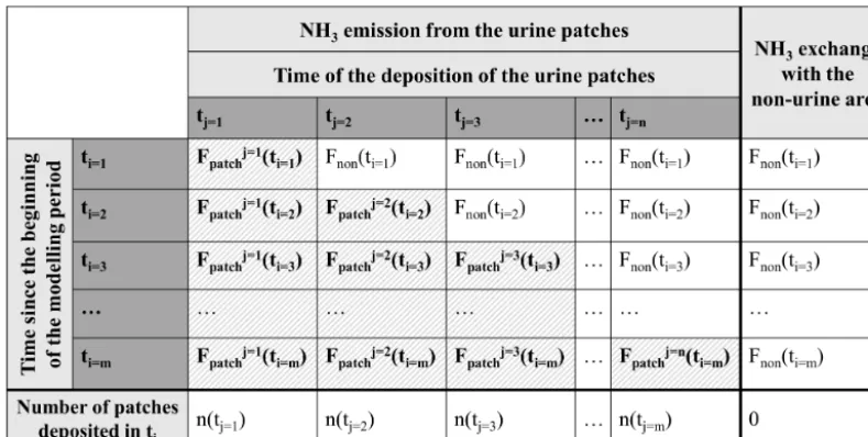
Figure 5.Schematic for the temporal development of NH3fluxes (in everyith time step,ti)as derived by GAG_field.Fpatchj (ti)stands for the NH3flux from the urine patches deposited in thejth time step (tj), andFnon(ti)stands for the NH3flux from the non-urine area. The
bottom row shows how many urine patches were deposited in the givenjth time step (n(tj)). Fluxes with striped background are calculated by GAG_patch, and the fluxes with clear background are calculated by a modified version of GAG_patch for non-urine area (explained in the text).
mis the number of the time steps in the modelling period). In this matrixiindex denotes the time step for which the given flux is derived and j shows the time step when the patches were deposited. In this way,Fnetin theith time step (ti)can
be expressed by Eq. (5).
The first term in the numerator of Eq. (5) represents the NH3emitted by the non-urine area: the NH3exchange flux over the non-urine area (Fnon)multiplied by the size of this area (Anon). The second term in the numerator equals to the total NH3emitted from the urine patches, whereFpatchj is the emission flux from the urine patches deposited in thejth time step, andn(tj)is the number of the patches deposited in the
same time step. To calculateFnet, the sum of the two has to be divided byAfield:
Fnet(ti)=
Fnon(ti) Anon(ti)+ m
P
j=1
Fpatchj (ti) n tjApatch
Afield . (5)
In the non-urine area, in the absence of any consider-able nitrogen input, the soil chemistry is practically undis-turbed. Thus, for the non-urine area a modified version of GAG_patch was applied in which constant soil chemistry was assumed. Based on this,Fnon was derived in the same way asFt, the net NH3flux over a urine patch in GAG_patch, described by Eqs. (1)–(7) in Móring et al. (2016), together with the following simplifications:
– Because over the non-urine area undisturbed soil istry is assumed, the dynamic simulation of soil chem-istry in GAG_field is not needed. Therefore, the origi-nal version of the two-layer canopy compensation point
model by Nemitz et al. (2001) is used. While dynamic simulation of undisturbed soil chemistry would be a useful avenue for further research, it is not addressed in the present study. The model by Nemitz et al. (2001) includes only the original compensation point on the ground (χg), instead of the soil resistance and compen-sation point in the soil assumed for GAG_patch. As a consequence, for the non-urine area the equation in GAG_patch for the NH3 emission from the soil (Fg) changes to
Fg=
χg−χz0 Rac+Rbg
, (6)
whereχz0 represents the canopy compensation point, and Rac and Rbg stand for the aerodynamic tance within the canopy and the quasi-laminar resis-tance at the ground, respectively (see the applied re-sistance model in Fig. S1 in the Supplement). For the parametrization of these variables in GAG_patch see Móring et al. (2016).
χg=
161 500 Tsoil
×exp
−10 380
Tsoil
×0g. (7)
– Since over the non-urine area no N input is assumed, for the emission potential of the stomata (0sto), instead of applying a decay function, like in GAG_patch, it was treated as constant (Sect. 3.2.3).
The size ofAnonin the giventi time step is the area of the
field that is not covered by any urine patches (assuming no overlap):
Anon(ti)=Afield−
i X
j=1
n tjApatch, (8)
wheren(tj)(Eq. 9) is the number of the urine patches
de-posited in thejth (hourly) time step. This can be expressed as the product of the animal density on the field intj(AD(tj),
animals ha−1),Afield(ha) and the daily UF (urinations day−1 animal−1), divided by 24 h:
n tj=
(AD(tj)×Afield×UF)
24 . (9)
Finally, Fpatchj (ti) was determined by Eq. (10), which
ex-presses that before the deposition of the urine patch, the area is handled as non-urine area (first condition), and afterwards GAG_patch calculates the net NH3flux over the urine patch (Ft(ti), second condition):
Fpatchj (ti)=
Fnon(ti) Ft(ti)
ifi < j
otherwise. (10)
When calculatingFt(ti)a slight modification is also required
compared with the GAG_patch model, regarding the urea added with a single urination (Uadd). At field scale it has to be considered that during the modelling period urine patches may be deposited at the same time as a rain event occurs. A rain event
i. will dilute the incoming urea solution, and
ii. may lead to the maximal water content (BH2O(max)) in the NH3source layer. In the formulation of GAG_patch this means that for the incoming liquid there is no more soil pore to fill, i.e. there is no infiltration. Therefore, when a urine patch is deposited while the water content is atBH2O(max), this will result in no N input to the sys-tem and consequently, no NH3emission from the soil. To address point (i), it has to be noted that although over the non-urine area GAG_field does not simulate the dy-namic, temporal evolution of the TAN budget and the soil pH (a constant 0g is used as noted above), it does account for the changes in water budget (BH2O)in the source layer.
Therefore, the water budget for the non-urine area (simu-lated by the modified version of the GAG_ patch as described above), right before thejth patch deposition (BHj
2O(ti=(j -1))), can be updated by GAG_ patch in the next time step (BHj
2O(ti=j )). Although the effect of dilution is treated in GAG_patch, it is defined only for the first time step, when urine is applied to the surface. This means that in Móring et al. (2016)Uaddwas not defined as a function of time. There-fore, in the field-scale model, where urine patches are de-posited in every time step,Uaddwas calculated for all of the urine patches deposited in everytjas
Uadd(tj)=cDilN tj
BH2Oj ti=(j )−BH2j O ti=(j−1)
, (11) where the diluted N concentration in the mixture of rain wa-ter and urine (cNDil, Eq. 12) equals to the total amount of N in the urine (cN×Wurine)divided by the sum of the volume of the liquid phase (Wurine+Wrain(ti =j ), whereWraindenotes the volume of the infiltrating rain water):
cNDil(tj)=
c
NWurine Wurine+Wrain(ti=j)
. (12)
To avoid the possible error resulting from the second point, it was assumed that instead of no infiltration, a small amount of water is always allowed to penetrate to the soil. This amount was chosen to be 5 % ofBH2O(max), as shown in Eq. (13). This assumption is necessary since in reality in most of the cases there is infiltration to the soil (except after heavy rain or an elongated rain event); therefore, there is NH3emission from the soil even if the urine patch is deposited to a very wet soil. However, in this case, the NH3emission flux from the soil might be weaker for two reasons: (1) due to the soil wetness, the urine might dilute after its deposition, leading to a lower χp and (2) the high water content is associated with large soil resistance, leading to a weaker NH3emission flux. Therefore, the choice of 5 % ofBH2O(max) could be reasonably large to avoid zero soil emission, but reasonably small to represent the described effects:
BH2Oj ti=(j )−BH2Oj ti=(j−1)
≥0.05
×BH2O(max) . (13)
3.2 Data set used in the baseline simulations and model evaluation
3.2.1 Measurements
Table 2.Urine-, soil- and site-specific constants used in the evaluation of GAG_field. The source of the values that were not measured at the site are also indicated. P2002 and P2003 stand for the modelling periods in 2002 and 2003, respectively. Constants used in the model, but not mentioned here, were kept the same as defined for the baseline simulation with GAG_patch (Móring et al., 2016).
Model constants Value Source
(if not measured)
Urine-specific constants
Apatch(area of a urine patch) 40 dm2 Williams and Haynes (1994)
(average value)
cN(nitrogen content of urine) 11 g N dm−3 Whitehead (1995)
(average values) Wurine(volume of urine) 2.5 dm3
Soil-specific constants
θfc(field capacity) 0.37
θpwp(permanent wilting point) 0.192
θpor(porosity) 0.54
pH(t0)(initial soil pH) 4.95
0g(soil emission potential) 3000 Modelled
(Sect. 3.2.3) θ (t0)(initial volumetric water content) 0.356 (P2002)
0.24 (P2003)
Site-specific constants
Latitude 55.87◦
Longitude 3.03◦
Height above sea level 190 m
Afield(field area) 5.424 ha
0sto(stomatal emission potential) 500 Massad et al. (2010)
(average value)
UF (urination frequency) 10 animal−1day−1 Whitehead (1995)
(average values)
zw(height of wind measurement) 1 m
Number of cattle on the field 40, 17 (P2002)∗
50, 52 (P2003)∗ z(heights of NH3concentration measurements) 0.44, 0.96, 2.06 m
∗The dates when the number of animals changed in P2002 and P2003 were 28 August 2002 and 23 June 2003, respectively.
on the boundary of the two (Fig. 6). For the site, NH3 flux measurements are available for a number of years (2001– 2007). These fluxes were derived using the aerodynamic gra-dient method, which calculates the fluxes (Fχ)based on
mea-surements of the vertical gradient of NH3air concentration and micrometeorological variables (Eq. 14). In Eq. (14) χ denotes the NH3 air concentration measured at az height, whilst k,u∗, d, 9H andL stand for the Karman constant, friction velocity, displacement height, the stability function for heat and the Monin–Obukhov length, respectively: Fχ= −ku∗
∂χ
∂ln(z−d)−9H z−Ld
. (14)
Ammonia concentration measurements were conducted by using a high-resolution NH3 analyser, AMANDA (Ammo-nia Measurement by ANnular Denuder sampling with online Analysis, Wyers et al., 1993). During the sampling, gaseous NH3 is captured in a continuous flow rotating annular wet
denuder applying a stripping solution of 3.6 mM sodium hy-drogen sulfate (NaHSO4). The technique determines the air concentration of NH3online by conductivity detection (Mil-ford et al., 2001). The concentration gradients were obtained from concentration measurements at three heights: 0.44, 0.96 and 2.06 m.
The meteorological input variables that are required for a simulation with GAG_field are the same as for GAG_patch. From these, air and soil temperature (Tair and Tsoil), rela-tive humidity (RH), precipitation (P ), atmospheric pressure (p), global radiation (Rglob), wind speed (u), wind direction (udir) and sensible heat flux (H ) were observed at Easter Bush. For further details on instrumentation see Milford et al. (2001). Since photosynthetically active radiation (PAR, µmol m2s−1)was not measured at the site, it was calculated fromRglobas shown in Eq. (15). According to Emberson et al. (2000), PAR is 45–50 % ofRglob(0.475 in Eq. 15), and it is expressed in µmol m−2s−1(to the unit ofR
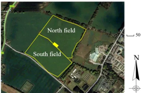
Figure 6.Satellite photo of the Easter Bush site. The map was gen-erated by Google Maps, indicating the two halves of the field and the place of the instruments on the border of the two denoted by the small yellow rectangle. (The figure is taken from the metadata file by CEH.)
conversion factor of 4.57 should be applied). The measured input data are illustrated in Figs. S2 and S3.
PAR=Rglob×0.475×4.57 (15)
3.2.2 Processing of the measured data for model application
For the baseline simulation and model evaluation (Sect. 4.1), a subset of the measurement data for 2001–2007 was selected that fulfilled the following criteria:
1. there were animals on the field;
2. grazing started at the beginning of the modelling period; 3. there had been no grazing, fertilizer spreading or grass
cutting in the week before the grazing started;
4. there are no significant gaps in the meteorological input data;
5. flux measurements are available for validation.
The second criterion is important because NH3fluxes over the field can be affected by emission from urine patches de-posited earlier. If the model does not account for these, it may underestimate the fluxes. The management practices listed in the third criterion can also affect the NH3exchange in a given time step, as well as fertilization can considerably affect the chemical balance of the soil. The latter would conflict with the model assumption that urine patches are deposited to a non-affected soil. The fourth criterion is necessary because a continuous input data set is needed for a simulation, since within GAG_patch the TAN, the water and the H+budgets in a given time step are dependent on the values in the previous time.
As a result of the filtering, two suitable time periods were found: 26 August 00:00–3 September 2002 06:00 and 20 June 00:00–25 June 2003 05:00. These periods are hence-forth referred to as P2002 and P2003, respectively. In both time intervals cattle were grazing on the South Field. Their number over the two modelling periods is indicated in Ta-ble 2.
To prepare the measured data sets for the hourly model application, firstly, the flux measurements were assessed for stability of the AMANDA instrumentation record with peri-ods of obvious instrument malfunction and gaps in data re-moved (Móring, 2016). All data were then averaged to an hourly time resolution. The time resolution of the ambient air concentration (χa),u,Tair andFχ (all at 1 m height) as
well asTsoil was 15 min, whilst it was 30 min for p,Rglob and RH. Secondly, in the resulted averaged time series (ex-cept inFχ)gap-filling was carried out. Data were missing
from theχadata set for the simulation for P2002:
– over 27 August 13:00–28 August 13:00,
– on 2 September at 23:00.
The individual gap was interpolated from the values from the previous and next time step, whilst over the long period of missing data inχa(25 consecutive hourly time steps), the values were replaced by the average of the measured values ofχa over P2002 (1.71 µg m−3). In P2003 a single, hourly wind speed was missing at 01:00 on 25 June, which was in-terpolated based on the data in the neighbouring two time steps.
In the third step of data processing, the measured fluxes were filtered according to the wind direction. As mentioned above, animals were grazing on the South Field and the fluxes were measured at the border line of the two fields (Fig. 6). Therefore, to distinguish the fluxes over the investi-gated part of the field, only the fluxes were used in the com-parison that were associated with wind from the direction of the South Field, between 135 and 315◦. The wind blew from this direction most of the time. In the two modelling periods in P2002 and P2003 the wind direction was the opposite in 7 and 15 % of the hourly time steps, respectively.
In addition, a quality check was carried out on the mea-sured flux data set, distinguishing the time periods with low wind and strong stability. A flux measurement was consid-ered robust if it met all of the following criteria:
– according to the footprint analysis, the field contributed at least 67 % to the measured flux,
– u∗> 0.15 m s−1for at least 45 min, – L−1< 0.2 m−1and
– u> 1 m s−1.
Finally, although the NH3concentrations measured in the time steps withudirfrom the North Field represent the con-centration in the North Field, in order to preserve continuity in the input data, these values were kept in the data set. Con-sidering the relatively small number ofudirvalues from the direction of the North Field, this choice is not anticipated to result in large errors in the NH3flux simulations.
3.2.3 Model constants
The main urine-patch-specific constants defined by Móring et al. (2016) for GAG_patch are the soil buffering capacity (β=0.021 mol H+(pH unit)−1dm−3) and the thickness of the NH3source layer (1z=4 mm); these were not changed in the model experiments with GAG_field. The other field-, urine- and site-specific constants together with their sources are listed in Table 2.
For the constant0sto,for the non-urine area of the field, where no considerable N input is assumed, the values from the emission potential inventory by Massad et al. (2010) for unfertilized grasslands were averaged. Because in the refer-enced inventory there were no0gestimates for non-fertilized grasslands, it was defined during preliminary simulations with GAG_field over a time interval when the grassland was not disturbed by any kind of management practice (grazing, fertilizer spreading or grass cutting). The period of 1 June 00:00–8 June 2003 16:00 fulfilled these criteria. These pre-liminary model experiments indicated a reasonable agree-ment between the measured and simulated NH3fluxes with a 0gof 3000 (see Fig. S4). Therefore, this value of0gwas ap-plied in the baseline simulations with GAG_field. To inves-tigate the model sensitivity to this choice of0g, a sensitivity analysis was carried out in Sect. 4.2.2.
3.3 Methods used in the sensitivity analysis
3.3.1 Perturbation experiments
Similarly to the model perturbation experiments carried out with GAG_patch (Móring et al., 2016), a sensitivity analysis of GAG_field to the regulating model parameters (Sect. 4.2.1–4.2.4) was performed. In addition to the param-eters that were investigated for GAG_patch (1z; β; REW, readily evaporable water;θfc, field capacity;θpwp, permanent wiling point),0sto,0g, pH(t0)(soil pH before urine deposi-tion), χa LAI (leaf area index) andh(canopy height) were also examined. The values ofθfcandθpwpexpress the maxi-mum and the minimaxi-mum volumetric water content in the soil, including the NH3source layer. For a detailed description of REW, see Móring et al. (2016).
The perturbation experiments were carried out as fol-lows. The investigated parameter was modified with±10 and ±20 %, while the other parameters were kept the same. In the case of the perturbation experiments for χa, theχa was modified by ±10 and±20 % of its average over both
peri-ods. These average concentrations in P2002 and P2003 were 1.73 and 1.51 µg NH3m−3, respectively. At the end of every simulation, the total NH3exchange (6Fnet)was calculated by summing the modelled hourly NH3 fluxes in the given modelling period. The difference compared with the baseline simulations was expressed in two ways. Firstly, it was calcu-lated as the percentage of6Fnetin the baseline model inte-grations (127 and 403 g N net emission for the whole field in the baseline simulations for P2002 and P2003, respectively), denoted as Sensnet. Secondly, the differences were derived as the absolute average hourly change, i.e.6Fnetin the actual perturbation experiment minus6Fnetin the baseline simula-tion, divided by the length of the modelling periods (199 and 126 h in P2002 and P2003, respectively).
In addition to the percentage differences for the whole field, similarly, the proportional change (Senspatch)in the to-tal NH3emission was calculated separately for the area cov-ered by the urine patches (6Fpatch)as well. In the baseline simulations, the total NH3emission from the urine patches were 717 and 846 g N in P2002 and P2003, respectively. Fi-nally, forβ,θfc, andθpwp,the percentage differences in the
total NH3emission (6Fpatchsingle)were calculated for every sin-gle urine patch deposited over both modelling periods, de-noted as Senssinglepatch.
When the results from the sensitivity analysis for GAG_field and GAG_patch are compared (the latter carried out by Móring et al., 2016), differences can occur for three reasons:
1. in GAG_field the total net NH3exchange consists of not only the total NH3emission over the urine patches but also the total net NH3exchange over the non-urine area;
2. in GAG_field multiple urine patches are deposited in ev-ery time step, whilst in GAG_patch a single urine patch is simulated;
3. the two models were applied for two different sites with different circumstances: GAG_field was applied for a grazed grassland at Easter Bush, Scotland, and GAG_patch was evaluated for a grassland at Lincoln, New Zealand.
3.3.2 Further methods used in the sensitivity analysis
As explained in Sect. 2.2.2, forcN,Apatchand UF constant, average values were applied in the baseline simulations with GAG_field. However, in reality these parameters can vary between different animals, and between different urination events as well. To examine the model uncertainty caused by these model assumptions, firstly, a sensitivity analysis was carried out (Sect. 4.2.5) applying the minimum and the max-imum of these parameters as suggested in the literature (Ta-bles 1 and 2; 20 g N dm−3for c
Nfrom Whitehead, 1995).
Since the results indicated that the largest uncertainty is coupled with cN (Sect. 4.2.5) in the case of this parameter further examinations were carried out. In natural conditions, even within an hour, several different urine patches are de-posited over the field. For example, calculating with the low-est animal number on the field in the baseline experiment with GAG_field (17 from Table 2) and the minimal UF (eight urinations day−1cattle−1, from Table 1), there were at least five urine patches deposited in an hour. When the number of urine patches is high enough, it can be assumed that the over-allcNof all the urine deposited in a given hour is character-ized by the average of thecNvalues related to the individual urination events. This can be expressed by Eq. (16), in which cAveN (tj)represents the average N concentration in the time
step tj, thecNk(tj)stands for the N content associated with
the kth urine patch intj, andn(tj)is the number of urine
patches deposited intj.
In the baseline simulations with GAG_field,cAveN was as-sumed to be 11 g N dm−3over the whole modelling period; therefore, it was examined how the model responds to a value of cNAve, which is calculated in every time step according to Eq. (16). To approach this task, firstlyckN values have to be randomized for every urination event from an estimated sta-tistical distribution ofcN.
Li et al. (2012) fitted a log-normal distribution (Eq. 17) to acNdata set, originating from the observation of two Ab-erdeen Angus steers over three 24 h periods (Betteridge et al., 1986). In Eq. (17)σandµare the scale parameters of the dis-tribution. These, in the fitted distribution by Li et al. (2012), were σ=0.786 and µ=1.154. The arithmetic mean ofcN calculated from these values (Eq. 18) was 4.33 g N dm−3. In the study of Li et al. (2012), the findings were applied for cows, assuming that the distribution ofcNis similar with the sameσ, but a higher meancN. Based on these, from Eq. (18), Li et al. (2012) derivedµof the new distribution for cows and from this they generated a series of samples forcN.
cAveN tj= n(tj)
P
k=1 ckN tj
n tj
. (16)
D (cN)= 1 cNσ
√ 2πe
−(lncN−µ)
2
[image:11.612.325.526.63.249.2]2σ2 , (17)
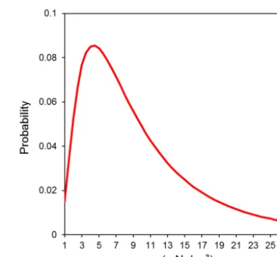
Figure 7.Probability density function of the log-normal distribution generated for the distribution of the nitrogen content of urine (cN).
The scale parameters areσ=0.786 andµ=2.089.
mean(cN)=eµ+ σ2
2 . (18)
To test the uncertainty coupled tocN in GAG_field, the fol-lowing steps were carried out. Firstly, folfol-lowing the method described by Li et al. (2012), based on Eq. (18), a new distribution of cN was obtained, assuming a mean cN of 11 g N dm−3, andσ=0.786. In this way, the scale param-eter µ was found to be 2.089. The resulted distribution of cNis depicted in Fig. 7. Secondly, in every time stepcNk val-ues were randomized from the resulted distribution, and from these,cAveN was derived based on Eq. (16). This resulted in a time series ofcAveN values. In total, 30cNAvetime series were generated for both experimental periods (P2002 and P2003) and simulations were performed with GAG_field, for all of these time series.
Finally, in order to investigate the model response of GAG_field to a constant value of soil pH, model experi-ments were performed with different constant values of soil pH (Sect. 4.2.6).
4 Results
4.1 Model results derived by GAG_field
Figure 8.NH3fluxes simulated by GAG_field against the measured NH3fluxes in P2002(a)and P2003(b). Green and blue dots represent
the data for all time steps when measured fluxes were available. The green dots indicate only those time steps in which the measured flux was considered robust as shown in Fig. 9 (in(a), the remaining data points on 27 August 2002 were also excluded as explained in Sect. 4.1.1). The figures show the fitted lines to the data points (thick black line for all of the data points, green dashed line for the green data points) in comparison with the 1:1 line (red line). The statistics indicated are the equation of the fitted lines (y), the Pearson correlation (R), the relative mean squared error (RMSE) and the level of significance of the relationship between the measured and modelled values (p) in the colour of the corresponding fitted line.
4.1.1 Baseline simulations and model evaluation
In the case of P2002, although the model statistics imply a weak model performance (Fig. 8a), the visual comparison of the modelled and measured NH3exchange (Fig. 9a) suggests a broad accordance between the two data sets. The model captures the characteristic daily variation of NH3 exchange detected over the period 31 August–2 September, with the magnitudes of the modelled and measured generally within 50 ng m−2s−1. A larger difference occurred on 2 Septem-ber when the model clearly underestimated the observations. Discrepancies between the simulated and measured values can be also seen in the first 2 days of the modelling period and on the fourth day. Nevertheless, on these days the bottom NH3concentration sensor did not work; therefore, the relia-bility of the flux calculated based only on the concentration measurements at the middle and top level is less certain. In addition, according to the metadata, on 27 August, before the gap in the observed fluxes (Fig. 9a), the stripping solution of the denuder ran out. This could explain the last 2–3 very high measured values beforehand. When the last six values before this event as well as the less robust data were removed from the data set, the calculated statistics reflected a much more promising model performance.
Similarly to P2002, the model statistics imply a relatively low model performance (Fig. 8b) for P2003 as well; how-ever, according to Fig. 9b, the simulation generally agreed with the observations within 50 ng m−2s−1. Removal of the less robust data from the data set resulted in improved model statistics (Fig. 8b), suggesting a better agreement between
the model and the measurements. The match with the ob-served fluxes was especially close in the second half of 23 June. By contrast, the largest difference was found on 24 June, in the morning, when an emission peak was detected during the measurements at 04:00–08:00. Even though there was a midday peak also in the simulation, it occurred 6 h later than the maximum in the observation. The increase in measured fluxes on 24 June was linked to a period of high wind speed (with largest values between 04:00 and 08:00, as shown in Figure S3b). Although wind speed is included in the model, the larger effect on measured fluxes could im-ply a proportionately larger effect of turbulence on the fluxes (through atmospheric and within canopy resistances, see the parametrization in Móring et al., 2016) than estimated by the model. In addition, it should be noted that on 20 June be-tween 11:00 and 15:00 the NH3concentration denuder in the bottom height was not functioning properly, and afterwards it was not operating until 23 June 13:00 (in these periods only the remaining two denuders were considered), suggest-ing uncertainty in the measured data set.
4.1.2 Contribution of the urine patches to NH3 exchange over the field
ex-Figure 9.Comparison of the measured and modelled NH3fluxes in the modelling periods P2002(a)and P2003(b). The uncertainty of
the flux measurements is depicted as error bars. Yellow error bars indicate the cases where one of the three NH3concentration denuders were malfunctioning or not registering data at all. For these, the error was estimated as the average of the observed errors (red error bars) multiplied by an arbitrary factor of 2. A measured flux was considered to be robust if it met the criteria of the quality control for low wind speed and strong stability as described in Sect. 3.2.2.
periments, deposition would have occurred for most of the time. This illustrates the considerable effect of the presence of grazing animals on NH3exchange over grasslands.
The contribution to the NH3exchange flux was also inves-tigated for the groups of patches deposited in the different time steps (Fig. 11). The ensemble of the fluxes from the dif-ferent patches show a clear daily variation with NH3 emis-sion peaks at midday in both modelling periods. In P2002, these peaks became lower from the fourth day because after the third day instead of the initial 40 animals, only 17 cattle were grazing on the field, depositing fewer urine patches.
In the baseline experiment with GAG_patch, the first and highest peak in NH3emission occurred about 12 h after the urine application (Móring et al., 2016). By contrast, in the
current results using GAG_field (Fig. 11) it can be observed that in some cases the highest peak over an individually de-posited urine patch emerges more slowly, only 1 or 2 days af-ter the urination event. For example, in P2002 (Fig. 11a) from the urine patches deposited on the third day (orange lines) the highest emission occurred on the fourth day, or from the patches deposited on the sixth day (dark green lines) the max-imal flux was observed 2 days later. Further examples from P2003 (Fig. 11b) are the urination events on the second day (orange lines) from which the highest flux can be observed a day after.
[image:13.612.104.494.63.463.2]Figure 10.Simulated NH3exchange fluxes over the urine patches, the non-urine area and the whole field in the modelling periods P2002(a)
and P2003(b).
the fluxes originating from the urination events 6 days before (red lines) are comparable with those from urine patches de-posited 2 days before (dark green lines).
4.2 Sensitivity analysis to the regulating model parameters
In the following, first, the results of the perturbation experi-ments (Table 3) with GAG_field are discussed (Sect. 4.2.1– 4.2.4). Secondly, in Sect. 4.2.5 the uncertainty associated with cN, Apatch and UF is investigated. Finally, model ex-periments are presented in which GAG_field was tested with different constant values of soil pH (Sect. 4.2.6).
4.2.1 General remarks
Based on Table 3, some preliminary, general conclusions can be drawn. Firstly, a near-constant ratio of Sensnet and Senspatchcan be observed for the urine-patch-related param-eters. These are the parameters that are used in the formula-tion of GAG_field only for the urine patches:1z,β, REW, θfc,θpwpand pH(t0)(initial soil pH). These have an effect on the NH3exchange for the whole field only through the NH3 emission from the urine patches.
pa-Table 3.Results of the perturbation experiments with GAG_ field. The changes in the total NH3flux over the field as a response to a change (±10 and±20 %) in the listed model parameters where expressed as the percentage of the total NH3exchange in the baseline simulations
with GAG_field and in the brackets as the hourly change in the total net exchange over the whole field (g N h−1). Results are listed for both modelling periods, P2002 and P2003, separately for the whole field (Sensnet)and the urine patches (Senspatch). As a comparison, the results
of the sensitivity analysis carried out by Móring et al. (2016) for GAG_patch are also indicated (Senssinglepatch). In the column “Effect” the letters denote how the given parameters affect total NH3exchange in GAG_field: through the urine patches (P) or the non-urine area (N) or both.
Change in the total net flux in response to the perturbation
P2002 P2003 GAG_patch
Constants (x) Effect 1x Sensnet Senspatch Sensnet Senspatch Senssinglepatch
1z(thickness of the source layer) P −20 % −40 % −7 % −8 % −4 % −12 %
(−0.26) (−0.27)
−10 % −18 % −3 % −4 % −2 % −6 %
(−0.11) (−0.12)
+10 % +14 % +2 % +2 % +1 % +5 %
(+0.09) (+0.08)
+20 % +25 % +4 % −2 % −1 % +11 %
(+0.16) (−0.06)
REW (readily evaporable water) P −20 % 0 % 0 % −3 % −1.3 % −3 %
(0.0) (−0.08)
−10 % 0 % 0 % −1 % −0.6 % −2 %
(0.0) (−0.04)
+10 % 0 % 0 % +1 % +0.6 % +2 %
(0.0) (+0.04)
+20 % 0 % 0 % +2 % +1.2 % +4 %
(0.0) (+0.08)
pH(t0)(initial soil pH) P −20 % −173 % −31 % −79 % −38 % –
(−1.11) (-2.53)
−10 % −90 % −16 % −42 % −20 % –
(−0.58) (−1.36)
+10 % +96 % +17 % +48 % +23 % –
(+0.61) (+1.53)
+20 % +196 % +35 % +100 % +48 % –
(+1.25) (+3.21)
0sto(stomatal emission potential) N −20 % −3 % – −1 % – –
(−0.02) (−0.02)
−10 % −1 % – −0.3 % – –
(−0.01) (−0.01)
+10 % +1 % – +0.3 % – –
(+0.01) (+0.01)
+20 % +3 % – +1 % – –
(0.02) (+0.02)
rameters was negligibly small (under 1 % in absolute value). Therefore, the effect of1z, REW,θfc andθpwpon the total NH3exchange over a grazed field through the non-urine area can be ignored.
In essence, when1z,β, REW,θfc,θpwpor pH(t0)are per-turbed, the changes of the total exchange flux are attributed exclusively to the changes in the emission flux over the urine patches. Therefore, as shown in the following, for these pa-rameters the ratio of Sensnet and Senspatch is close to con-stant. Since the net NH3exchange over the whole field equals
the sum of the NH3emission from the urine patches and the NH3exchange over the non-urine area (Fig. 4), the total NH3 exchange over the whole field (6Fnet, Eq. 19) over a time in-terval is equal to the sum of the total NH3 exchange over the non-urine area (6Fnon)and the total NH3emission from the urine patches (6Fpatch). Therefore, based on Eq. (19), when a urine-patch-related parameter is perturbed, the result-ing differences (1F )in6Fpatchand6Fnetwill be the same.
X
Fnet=
X
Fnon+
X
[image:15.612.83.514.154.576.2]Table 3.Continued.
Change in the total net flux in response to the perturbation
P2002 P2003 GAG_patch
Constants (x) Effect 1x Sensnet Senspatch Sensnet Senspatch Senssinglepatch
0g(soil emission potential) N −20 % −54 % – −12 % – –
(−0.34) (−0.38)
−10 % −27 % – −6 % – –
(−0.17) (−0.19)
+10 % +27 % – +6 % – –
(+0.17) (+0.19)
+20 % +54 % – +12 % – –
(+0.34) (+0.38)
β(soil buffering capacity) P −20 % +94 % +17 % +50 % +24 % +1 %
(+0.60) (+1.61)
−10 % +46 % +8 % +24 % +11 % +1 %
(+0.29) (+0.77)
+10 % −43 % −8 % −22 % −10 % −1 %
(−0.28) (−0.69)
+20 % −84 % −15 % −41 % −20 % −1 %
(−0.53) (−1.31)
θfc(field capacity) P −20 % −360 % −64 % −153 % −72 % -18 %
(−2.30) (−4.88)
−10 % −190 % −34 % −85 % −40 % −7 %
(−1.22) (−2.71)
+10 % +211 % +37 % +96 % +46 % +6 %
(+1.35) (+3.07)
+20 % +448 % +79 % +191 % +91 % +9 %
(+2.86) (+6.09)
θpwp(permanent wilting point) P −20 % +364 % +64 % +157 % +75 % +9 %
(+2.32) (+5.03)
−10 % +173 % +31 % +76 % +36 % +5 %
(1.11) (+2.43)
+10 % −156 % −28 % −65 % −31 % −4 %
(−1.00) (−2.07)
+20 % −292 % −52 % −118 % −56 % −9 %
(−1.87) (−3.79)
χa(ambient atmospheric NH3 P, N −20 % +166 % +0.3 % +36 % +0.3 % –
concentration)* (+1.06) (+0.012) (+1.16) (+0.02)
−10 % +83 % +0.2 % +18 % +0.2 % – (+0.53) (+0.006) (+0.58) (+0.01)
+10 % −84 % −0.2 % −19 % −0.2 % –
(−0.53) (−0.006) (−0.61) (−0.01)
+20 % −167 % −0.3 % −38 % −0.3 % –
(−1.07) (−0.012) (−1.22) (−0.02)
Using1F, Senspatchand Sensnetcan be expressed as Senspatch=P1F
Fpatch
, (20)
Sensnet= 1F
P
Fnet
. (21)
Based on these, it can be clearly seen that the ratio of Sensnet and Senspatchequals the ratio of6Fpatchand6Fnet. These
ra-tios are 5.6 and 2.1 for P2002 and P2003, respectively, which is in accordance with the Sensnetand Senspatchvalues in Ta-ble 3.
Table 3.Continued.
Change in the total net flux in response to the perturbation
P2002 P2003 GAG_patch
Constants (x) Effect 1x Sensnet Senspatch Sensnet Senspatch Senssinglepatch
LAI (leaf area index) P, N −20 % −1.1 % +0.11 % +0.10 % +0.15 % –
(−0.007) (+0.004) (+0.003) (+0.010)
−10 % −.5 % +0.05 % +0.05 % +0.07 % – (−0.003) (+0.002) (+0.002) (+0.005)
+10 % +0.5 % −0.05 % −0.05 % −0.07 % –
(+0.003) (−0.02) (−0.002) (−0.005)
+20 % +1.1 % −0.11 % −0.10 % −0.14 % –
(+0.007) (−0.004) (−0.003) (−0.010)
h(canopy height) P, N −20 % −12 % −8 % −9 % −8 % –
(−0.08) (−0.28) (−0.28) (−0.51)
−10 % −6 % −4 % −4 % −4 % – (−0.04) (−0.14) (−0.13) (−0.25)
+10 % +4 % +4 % +4 % +4 % – (+0.03) (+0.13) (+0.14) (+0.26)
+20 % +6 % +7 % +8 % +7 % – (+0.04) (+0.26) (+0.26) (+0.49)
∗In both P2002 and P2003χ
awas changed by±10 and±20 % of the averageχairover each period as explained in Sect. 3.3.1.
On average, in P2003 and P2002, 21 and 8 urine patches were deposited in an hour, respectively. The ratio of the two, 2.625, is in agreement with the observed ratio in the hourly changes for P2002 and P2003.
Finally, based on the results of Table 3, it is clear that Sensnetis substantially affected by6Fnet. For example, when χa was perturbed by−20 %, the absolute changes in6Fnet were similar in P2002 and P2003 (+1.06 and+1.16 g N h−1, respectively); however, there was an enormous difference in the resulting Sensnet values (+166 and +36 %). This sug-gests that when the model behaviour is compared for P2002 and P2003, the Sensnet values can be interpreted only to-gether with the hourly absolute changes of6Fnet. To visually compare these absolute changes with the values in Fig. 9, the hourly average error of the measurements can be taken as a base:±2.86 and±2.46 g N in P2002 and P2003, respec-tively, after conversion from flux (ng NH3m−2s−1)to total emission for the whole field.
4.2.2 Sensitivity to1z, REW, pH(t0),0stoand0g,χa, LAI andh
According to Table 3, compared with the other patch-related parameters, for GAG_field,6Fnetturned out to be the least sensitive to the changes in1zand REW. The Senspatchvalues were similar in the case of the perturbation experiments with GAG_patch, with an overall, slightly stronger sensitivity than was found in the case of GAG_field.
In the case of pH(t0),6Fnetwas found to be very sensitive to the ±10 and±20 % modifications (Table 3). However, it
has to be pointed out that these changes in the value of pH(t0) (±0.5 unit for a±10 % modification and±1 unit for±20 %), can be considered as a large increase in the soil pH, taking into account that during intensive urea hydrolysis 2–3 units change can be expected (Fig. 12).
The constant0stoand0soilaffect NH3exchange over the whole field exclusively through its effect on the NH3 ex-change over the non-urine area. As the results show (Table 3), the model is only slightly sensitive to0sto,while0gcan have a considerable effect on NH3exchange. As can be seen, for 0sto the resulting changes in6Fnet, depending on the mod-elling period, are about 5–15 % of the perturbations applied to0sto. This means that if a 5 times larger0sto(+400 % per-turbation, assuming a soil richer in N) was used in the model runs, the resulting 6Fnet would be about 20–60 % larger, with an overall hourly difference of 0.4 g N.
As forχair, in Table 3 the percentage differences for P2002 over the whole field suggest a significant effect on6Fnet. However, comparing the absolute hourly change to that for P2003, it can be concluded that the absolute influence was similar for the two periods. It can also be clearly seen that the absolute hourly changes over the urine patches are neg-ligibly small in both P2002 and P2003 compared to the ab-solute changes observed for the whole field, suggesting that χair affects6Fnetmainly through the non-urine area, rather than the urine patches.
Figure 11.Simulated NH3fluxes from urine patches deposited in the same time step in the modelling periods P2002(a)and P2003(b).
Each line indicates NH3fluxes from urine patches deposited in a given time step (expressed for the whole field), while the different colours
indicate the days of the urination events. The number above the plots show how many cattle were grazing in the given time intervals.
case, it has to be noted that the resulting percentage differ-ences are about half of the perturbations. This means that a canopy height of, for example, 5 cm, which is−83 % shorter than the h used in the baseline simulations, could lead to considerable changes in the NH3exchange flux, especially toward the end of the period when the grass is shorter on the field due to the continuous grazing.
4.2.3 Sensitivity toβ
Figure 12.Simulated soil pH in the NH3source layer under urine patches deposited in the same time step in the modelling periods, P2002(a)
and P2003(b)in the baseline experiments with GAG_field. The different colours indicate the days of the urination events. Each line indicates soil pH under urine patches deposited in a given time step, while the different colours indicate the days of the urination events.
Table 4.Results from simulations with GAG_patch, testing the effect of pH(t0)(initial soil pH),θfc(field capacity) andθpwp(permanent
wilting point) on the sensitivity of the total NH3emission toβ(buffering capacity). Input data were applied from the baseline simulation
with GAG_patch (Móring et al., 2016), except for the parameters denoted in the table with a different font style. Bold values are taken from the input data for the baseline simulations with GAG_field, and italics denote a situation when the water content was assumed to be halfway between the field-scale values ofθfcandθpwp. The sensitivity was expressed as the percentage difference in the original NH3emission
derived with the given model settings with GAG_patch (listed also in the table for every model experiment).
Model Model settings Original Response of emission
experiment emission to a change inβby
pH(t0) θfc θpwp (g N) −20 % −10 % +10 % +20 %
A 4.95 0.40 0.10 1.5 g +5 % +2 % −2 % −5 %
B 6.65 0.37 0.19 0.9 g +3 % +1 % −1 % −2 %
C 4.95 0.37 0.19 0.6 g +11 % +5 % −5 % −10 %
[image:19.612.130.469.604.699.2]leaving behind the high peaks associated with the events of dew fall (Figs. 13a and 14a). These results suggest that Senssinglepatch is affected by the volumetric water content at the time of the deposition of the urine patch. Furthermore, com-paring the patch sensitivities illustrated in Figs. 13b and 14b with those in Table 3 reported by Móring et al. (2016), a large difference occurs over the urine patches observed at the two different sites, Lincoln (NZ) and Easter Bush (UK). There-fore, in the following, two questions are investigated:
– What causes the difference between the patches at the two different sites?
– What causes the high peaks in the sensitivity toβ? For both questions, the general model behaviour was exam-ined through a series of model experiments with GAG_patch (Table 4).
In Móring et al. (2016), the H+ ion budget depends on the H+ ion consuming and producing processes re-lated to the products of urea breakdown. On top of these, the effect of the buffers in the soil is expressed with an additional term: (pH(ti)−pH(ti−1))×βpatch, where βpatch=β×Apatch×1z. Based on these, the main factors that can regulate the governing role of buffering in the evo-lution of soil pH in the NH3source layer and subsequently, NH3exchange are
1. pH(ti)−pH(ti−1), and 2. βpatch.
Considering point (1), if pH(t0) is low, i.e. [H+] is high, during urea hydrolysis more H+ ion can be consumed.
This results in a larger increase in soil pH shortly after the urine patch deposition. In the baseline simulations with GAG_patch and GAG_field, pH(t0)was 6.65 and 4.95, re-spectively. In Fig. 12 it can be observed that in most of the urine patches deposited in the baseline simulations with GAG_field, the difference between the initial and maximum soil pH was about 3 units, whilst in the case of the baseline experiment with GAG_patch (with the higher pH(t0))it was only 2 (Móring et al., 2016).
These larger changes in soil pH generate a larger buffer-ing effect ((pH(ti)−pH(ti−1))×βpatch), i.e. a larger term in the H+ budget. This means that in the GAG_field sim-ulations, this term has a stronger effect in the H+ budget. Consequently, whenβ is modified (throughβpatch), the sys-tem gives a stronger response, which means that the model is more sensitive to the perturbation of β. This was con-firmed in the model experiment A (Table 4). In this simu-lation, GAG_patch was run with the initial pH of 4.95 used in the baseline simulation with GAG_field. Although the re-sponse of NH3exchange was relatively weak to the modifi-cations ofβ, it was stronger than in the original perturbation experiment for GAG_patch (Table 3).
Regarding point (2), the definition ofβpatchexpresses the buffering effect of the solid material of the soil on the liq-uid content. As can be seen from the formulaβpatch=β× Apatch×1z,βpatchdepends clearly on1z, but it does not de-pend on the liquid content of the soil. This means that in the model, in a source layer with the same1z, the same buffering effect takes place even if less urine stored in it. In a smaller amount of urine, the H+ion budget (expressed in mol H+)and the variations in it are proportionally smaller too. Therefore, the governing role of the same buffering ca-pacity in the case of a smaller amount of urine becomes stronger, resulting in a stronger model sensitivity toβ.
The maximum volume of urine that can be stored in the NH3 source layer (θurine) can be calculated as the differ-ence betweenθfcandθpwp. The values ofθurine in the base-line experiments with GAG_field and GAG_patch were 0.18 and 0.3, respectively. This, based on the above consideration, suggests a stronger response in6Fpatchsingle to the perturbation of β for the GAG_field experiments than the GAG_patch experiment. This effect was explored in the model exper-iment B (Table 4), in which the baseline simulation with GAG_patch was performed withθfcandθpwpapplied from the baseline experiment with GAG_field (Table 2). The re-sults show a small difference in6Fpatchsinglein response to the change ofβ, but it is still larger than in the sensitivity anal-ysis carried out for the baseline simulation with GAG_patch (Table 3), supporting the effect described above. When the influence of pH(t0) and the soil water content characteris-tics were examined together (model experiment C, Table 4), their effect added up, reaching a±10 % difference in6Fpatch whenβwas modified by±20 %.
The model was tested also with a higherθpwp(model ex-periment D, Table 4), assuming that half of the available space for urine in the model soil pore is filled with water, allowing only half ofθurine to infiltrate. This can represent a situation on the field when a urine patch is deposited af-ter a rain event, when only half of the soil pore is empty. As expected, due to the smaller amount of urine, with this mod-ification the sensitivity toβbecame even stronger.
Overall, these findings show that the difference in Senssinglepatch in response to the perturbations ofβ between the GAG_field and GAG_patch simulations are mainly caused by the difference inθfcandθpwpas well as pH(t0)at the two different sites. Furthermore, the above results highlight that the sensitivity of6Fpatchsingletoβcan vary between wide ranges over the individual urine patches on the same field, depend-ing on the water content of the soil at the time of the given urination event.
4.2.4 Sensitivity toθfcandθpwp
Figure 13.Results of the perturbation experiments for every single urine patch deposited over P2002. The results are shown in comparison with the volumetric water content of the soil at the time of urine patch deposition, changing in response to the events of precipitation and dewfall(a). The investigated parameters were the buffering capacity (β,b), the field capacity (θfc,c) and the permanent wilting point (θpwp, d). In panels(b)–(d), a point represents the percentage difference in the total NH3emission from the urine patch deposited in the given time