Ames Laboratory Accepted Manuscripts Ames Laboratory
10-15-2018
Calculation of critical nucleation rates by the
persistent embryo method: application to quasi
hard sphere models
Shang Ren
Iowa State University and Ames Laboratory, [email protected]
Yang Sun
Ames Laboratory, [email protected]
Feng Zhang
Ames Laboratory, [email protected]
Alex Travesset
Iowa State University and Ames Laboratory, [email protected]
Cai-Zhuang Wang
Iowa State University and Ames Laboratory, [email protected]
See next page for additional authors
Follow this and additional works at:https://lib.dr.iastate.edu/ameslab_manuscripts Part of thePhysics Commons
This Article is brought to you for free and open access by the Ames Laboratory at Iowa State University Digital Repository. It has been accepted for inclusion in Ames Laboratory Accepted Manuscripts by an authorized administrator of Iowa State University Digital Repository. For more information, please [email protected].
Recommended Citation
Ren, Shang; Sun, Yang; Zhang, Feng; Travesset, Alex; Wang, Cai-Zhuang; and Ho, Kai-Ming, "Calculation of critical nucleation rates by the persistent embryo method: application to quasi hard sphere models" (2018).Ames Laboratory Accepted Manuscripts. 390.
Calculation of critical nucleation rates by the persistent embryo method:
application to quasi hard sphere models
Abstract
We study the crystal nucleation of the Weeks–Chandler–Andersen (WCA) model, using the recently introduced persistent embryo method (PEM). The method provides detailed characterization of pre-critical, critical and post-critical nuclei, as well as nucleation rates that compare favorably with those obtained using other methods (umbrella sampling, forward flux sampling or seeding). We further map our results to a hard sphere model allowing comparison with other existing predictions. Implications for experiments are also discussed.
Disciplines
Physics
Authors
Shang Ren, Yang Sun, Feng Zhang, Alex Travesset, Cai-Zhuang Wang, and Kai-Ming Ho
1
Calculation of Critical Nucleation Rates by the Persistent Embryo
Method: Application to Quasi Hard Sphere Models
Shang Ren1,2, Yang Sun2*, Feng Zhang2*, Alex Travesset1,2, Cai-Zhuang Wang1,2, and Kai-Ming Ho1,2,3
1Department of Physics and Astronomy, Iowa State University, Ames, Iowa 50011, USA
2Ames Laboratory, U.S. Department of Energy, Ames, Iowa 50011, USA
3Hefei National Laboratory for Physical Sciences at the Microscale and Department of Physics,
University of Science and Technology of China, Hefei, Anhui 230026, China
Abstract
We study crystal nucleation of the Weeks-Chandler-Andersen (WCA) model, using the recently introduced Persistent Embryo Method (PEM). The method provides detailed characterization of pre-critical, critical and post-critical nuclei, as well as nucleation rates that compare favorably with those obtained using other methods (umbrella sampling, forward flux sampling or seeding). We further map our results to a hard sphere model allowing to compare with other existing predictions. Implications for experiments are also discussed.
1. Introduction
The nucleation of a crystal out of a supercooled fluid is a fundamental process of enormous
complexity. Even though Classical Nucleation Theory (CNT) was proposed almost a century ago1,
it is only recently, with the development of powerful computers, that parameter-free predictions
have become possible. Hard sphere (HS) models2,3 and other closely related systems4–8 have
provided fertile test grounds on which implementations of CNT can be tested: Brute force
Brownian dynamics (BD)4,5, forward flux sampling (FFS)2,4,6, umbrella sampling (US)4,
metadynamics and seeding method7. Despite its obvious theoretical motivations, these models are
also of considerable experimental interest, as they approximately describe colloidal dispersions9–
2 11. Experimental nucleation rates, however, remain in significant disagreement with most existing
theoretical predictions using these simple models4,12.
Recently, we have introduced the Persistent Embryo Method (PEM)13 and applied it to the
investigation of the nucleation of pure Ni and binary CuZr by all atom MD simulations. In this
paper, we demonstrate that PEM is an efficient method by applying it to the
Weeks-Chandler-Andersen (WCA) model14, assuming the validity of CNT. As we describe further below, PEM can
measure the nucleation rate in the low-density regime and does not make any geometrical
assumption on the shape of nucleus. Moreover, PEM can obtain the unbiased configuration of the
critical nucleus. We expect that PEM will become the method of choice as the optimal
implementation of CNT for certain problems. Furthermore, given the current disagreements
between nucleation rates as measured in experiments or calculated by theory, new techniques are
crucial, in that they provide additional insights on the origins of such discrepancies.
This paper is organized as follows: in Sec. 2 we present the WCA model, including the description
of Brownian dynamics and order parameter. In Sec. 3 we show the method and discuss the
calculation of other necessary quantities, such as the chemical potential. Sec. 4 describes the
persistent-embryo method (PEM) and Sec. 5 describes the determination of attachment rate. In
Sec. 6, we derive the rate equation and present our predictions. In Sec. 7, we discuss our results
and compare them with existing estimates obtained by other methods. A comparison with
experimental results is also included. The conclusions are left for Sec. 8.
3
To relate our calculation to experiments9–11, and also to compare with previous computational
work4–6, we performed Brownian dynamics (BD) simulations of N particles interacting with the
WCA potential14:
𝑈𝑈𝑊𝑊𝑊𝑊𝑊𝑊(𝑟𝑟) =�4𝜀𝜀 �� 𝜎𝜎 𝑟𝑟�
12
− �𝜎𝜎𝑟𝑟�6 +14� 𝑟𝑟 ≤216𝜎𝜎
0 𝑟𝑟> 216𝜎𝜎
where 𝜎𝜎 is the unit of length and 𝜀𝜀 is the unit of energy. The WCA model is a softer version of the
HS system14, and it is possible to define a mapping from the WCA model to the HS model, as we
discuss further below.
Brownian dynamics is the overdamped limit of Langevin dynamics. In Brownian dynamics, the
equation of motion of particle i is:
𝑑𝑑𝒓𝒓𝒊𝒊 𝑑𝑑𝑑𝑑 =
1
𝑀𝑀𝑀𝑀[−∇𝑖𝑖𝑈𝑈+𝑾𝑾𝒊𝒊(𝑑𝑑)] (1)
where 𝑀𝑀 is the friction coefficient with units of inverse time. 𝑾𝑾𝒊𝒊(𝑑𝑑) is the stochastic force and M
is the mass of the particle, which is subject to a conservative force −∇𝑖𝑖𝑈𝑈. The stochastic force is
correlated according to the dissipation-fluctuation theorem 〈𝑾𝑾𝒊𝒊(𝑑𝑑)𝑾𝑾𝒋𝒋(𝑑𝑑′)〉= 6𝑀𝑀𝑀𝑀𝑘𝑘𝐵𝐵𝑇𝑇𝛿𝛿𝑖𝑖𝑖𝑖𝛿𝛿(𝑑𝑑 −
𝑑𝑑′), where the 𝛿𝛿 is the Kronecker delta function and 𝑘𝑘𝐵𝐵 is the Boltzmann constant. The timestep of
the simulation is 0.0004 𝜏𝜏 (𝜏𝜏 is the LJ time unit which equals �𝑚𝑚𝜎𝜎2
𝜀𝜀 , where m is the unit of mass).
Note the Brownian time 𝜏𝜏𝐵𝐵 is defined as 𝜏𝜏𝐵𝐵 = σ2
𝐷𝐷, where 𝐷𝐷 is the diffusion coefficient on the
Brownian motion determined by the Einstein relation 𝐷𝐷 =𝑘𝑘𝐵𝐵𝑇𝑇/𝑀𝑀𝑀𝑀. Following Kawasaki and
Tanaka5, we studied the WCA model at the reduced temperature 𝛽𝛽𝜀𝜀 = 40, i.e. 𝑇𝑇= 0.025 𝜀𝜀/𝑘𝑘𝐵𝐵.
For simplicity, both 𝑀𝑀 and 𝑀𝑀 were set to unity. Therefore, 𝐷𝐷 = 0.025 𝜎𝜎2
4
simulations were performed using the GPU-accelerated LAMMPS code15–17. Some of the results
were also tested using HOOMD-blue18,19.
Identification of fluid-like and solid-like particles was accomplished by the use of the
bond-orientational order parameter20,21, which is described below for the sake of completeness. For each
particle i, the bond-orientational order parameter is:
𝑞𝑞6𝑚𝑚(𝑖𝑖) =𝑁𝑁𝑏𝑏1(𝑖𝑖) × � 𝑌𝑌𝑙𝑙𝑚𝑚(𝑟𝑟⃗𝑖𝑖𝑖𝑖) 𝑁𝑁𝑏𝑏(𝑖𝑖)
𝑖𝑖=1
(2)
where 𝑌𝑌𝑙𝑙𝑚𝑚 are the spherical harmonics, 𝑟𝑟⃗𝑖𝑖𝑖𝑖 is the position vector of particle j regards to particle i,
and 𝑁𝑁𝑏𝑏(𝑖𝑖) is the number of nearest neighbors of particle i. The normalized bond-orientational order
parameter is:
𝑞𝑞�6𝑚𝑚(𝑖𝑖) =[∑ 𝑞𝑞6𝑚𝑚|𝑞𝑞 (𝑖𝑖) 6𝑚𝑚(𝑖𝑖)|2 6
𝑚𝑚=−6 ]1/2 (3)
A correlation between two particles (i, j) is defined by:
𝑆𝑆𝑖𝑖𝑖𝑖 = � 𝑞𝑞6𝑚𝑚(𝑖𝑖)𝑞𝑞6𝑚𝑚∗ (𝑗𝑗) 6
𝑚𝑚=−6
(4)
If 𝑆𝑆𝑖𝑖𝑖𝑖 exceeds a threshold, then the two particles are considered bonded. To compare with a
previous study4, we chose 𝑁𝑁𝑏𝑏(𝑖𝑖) as the number of particles within a cutoff of 1.5𝜎𝜎, and a threshold
value for 𝑆𝑆𝑖𝑖𝑖𝑖 of 0.7. We denote 𝜉𝜉 as the minimal number of connected neighbors for a particle to
be considered as solid. In our simulation, if a given particle has 6 or more connected neighbors, it
5
show later it leads to a significant uncertainty in the calculation of related physical quantities, as
we explore the case of 𝜉𝜉 = 8 and 9, and make an additional comparison with Filion et al.4.
3. Chemical potential differences
The chemical potential difference between solid and fluid (∆𝜇𝜇) is required for calculation of
nucleation rates by CNT. To compute ∆𝜇𝜇 , we make use of the Gibbs-Helmholtz integration:
∆𝜇𝜇 𝑇𝑇𝑓𝑓 =�
∆𝐻𝐻(𝑇𝑇) 𝑇𝑇2 𝑇𝑇𝑓𝑓
𝑇𝑇𝑚𝑚
𝑑𝑑𝑇𝑇 (5)
where ∆𝐻𝐻(𝑇𝑇) is the enthalpy difference between the solid and fluid under the target pressure, 𝑇𝑇𝑚𝑚
is the melting temperature, and 𝑇𝑇𝑓𝑓 is final target temperature. The NPT ensemble was applied to
calculate enthalpy (H). For a fixed density, we first ran a BD simulation at the target temperature
(𝛽𝛽𝜀𝜀= 40) to obtain the target pressure 𝑃𝑃𝑓𝑓 in the fluid for subsequent simulations. The target
pressure in different densities was presented in Table 1, in the reduced form. To perform the
constant pressure simulation for Brownian particles, we used the Berendsen barostat22. We ran
separate simulations with 4000 particles in a solid face-centered cubic (FCC) phase and a fluid
phase at the same temperature. We considered the FCC phase as it is well established that it has
the lowest free energy among all putative crystalline phases in HS system. Other possibilities, such
as body-centered cubic (BCC) and icosahedral phases, do not seem to play a role in the nucleation
of monodisperse HS system3. As a cross-check, we ran simulations with a BCC embryo and found
6
To prepare the supercooled fluid phase, we first melted a crystal at a high temperature and cooled
it down to the target temperature. The numerical integration was carried out using a chained
trapezoidal rule with the interval of temperature ∆𝑇𝑇= 0.0001 𝜀𝜀/𝑘𝑘𝐵𝐵.
The melting temperature, as a function of fluid density, is the lower limit of Gibbs-Helmholtz
integration. To determine the melting point, we ran BD simulation on a solid-fluid interface
generated by melting half of the initial crystal (FCC) structure. During the simulation, the periodic
boundary condition was applied, and we only allowed the length of the box in the direction
perpendicular to the interface to change, resulting in constant interfacial area, constant normal
pressure: NPxAT ensemble, with x being the perpendicular direction. A typical configuration of
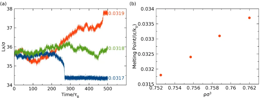
NPxAT simulation is shown in Fig. 1. We monitored the length of the simulation cell 𝐿𝐿𝑥𝑥 along the
x-direction to locate the phase transition at different temperatures: increasing of 𝐿𝐿𝑥𝑥 implies melting
7
Fig. 1: Typical configuration of NPxAT simulation. The central part is the crystalline phase, while the remaining fluid. Periodic boundary conditions were applied during simulation. 𝐿𝐿𝑥𝑥 is the length of simulation box along x-direction.
A typical measurement of the melting point is exemplified in Fig. 2: At 𝑇𝑇= 0.0319 𝜀𝜀/𝑘𝑘𝐵𝐵, the
simulation box expands, indicating that the solid is melting towards the fluid. At 𝑇𝑇= 0.0317 𝜀𝜀/𝑘𝑘𝐵𝐵,
the simulation box shrinks, implying that the fluid side is crystalizing towards the solid. Only at
𝑇𝑇= 0.0318 𝜀𝜀/𝑘𝑘𝐵𝐵, the box size stays around 35.7 𝜎𝜎 and both phases coexist. Therefore, this is the
melting temperature (within a 0.0001 𝜀𝜀/𝑘𝑘𝐵𝐵 precision) at a fluid density ρσ3 = 0.7525. All the
melting points thus obtained are shown in Fig. 2(b).
Fig. 2: (a) Lx as a function of temperature at 𝑇𝑇= 0.0317, 0.0318, 0.0319 𝜖𝜖/𝑘𝑘𝐵𝐵. (b) Melting point
as a function of reduced density (𝜌𝜌𝜎𝜎3).
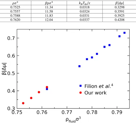
With the measured melting points and enthalpies, we compute the chemical potential differences
by Equation 5. A summary of thermodynamic properties is given in Table 1. In Fig.3, we compared
the reduced chemical potential differences with the results from Filion et al.4, obtained by a
[image:9.612.75.534.327.500.2]8
Table 1. Thermodynamic properties calculated at various reduced densities, including the reduced pressure (𝛽𝛽𝜌𝜌𝜎𝜎3), melting points (𝑘𝑘𝐵𝐵𝑇𝑇𝑚𝑚/𝜀𝜀) and reduced chemical potential differences (𝛽𝛽|𝛥𝛥𝜇𝜇|).
𝜌𝜌𝜎𝜎3 𝛽𝛽𝛽𝛽𝜎𝜎3 𝑘𝑘
𝐵𝐵𝑇𝑇𝑚𝑚/𝜀𝜀 𝛽𝛽|𝛥𝛥𝜇𝜇|
0.7525 11.34 0.0318 0.3298
0.7557 11.58 0.0324 0.3591
0.7588 11.83 0.0331 0.3925
0.7620 12.04 0.0337 0.4208
Fig. 3: The reduced chemical potential differences as a function of fluid density. The data from ref. 4 is also included in this figure.
4. The persistent embryo method (PEM)
Nucleation is described as a competition between the favorable fluid-to-crystal transition against
9
∆𝐺𝐺(𝑁𝑁) =𝑁𝑁∆𝜇𝜇+𝑠𝑠 �𝑁𝑁𝜌𝜌� 2 3
𝑀𝑀𝑖𝑖 (6)
where ∆𝜇𝜇(< 0) is the chemical potential difference. 𝑀𝑀𝑖𝑖(> 0) is the SFI free energy, and s is a
geometric factor that accounts for the possible non-sphericity of the critical nucleus.
During PEM simulation, the number of total particles was set to 13500. The NVT ensemble was
applied during PEM simulation. We first ran a BD simulation for 50,000 𝜏𝜏𝐵𝐵 at 𝜌𝜌𝜎𝜎3 = 0.7525 and
we did not observe a single nucleation event. PEM13 starts with the creation of a small embryo
consisting of a crystal of 𝑁𝑁0 atoms (𝑁𝑁0 ≪ 𝑁𝑁∗), where 𝑁𝑁∗ is the size of critical nucleus. We inserted
this embryo into the supercooled fluid and found that without any other modification, the embryo
quickly dissolves back into the fluid. We therefore attached each of the initial embryo particles to
a tunable spring while the other end of the spring is fixed to the embryo particle’s equilibrium
position, so that the embryo is prevented from shrinking and forced to grow. As the embryo grows,
springs are gradually softened so that at a size 𝑁𝑁𝑠𝑠𝑠𝑠(<𝑁𝑁∗) they are completely removed. This was
accomplished by parameterizing spring constants according to:
𝑘𝑘(𝑁𝑁) =�𝑘𝑘0𝑁𝑁𝑠𝑠𝑠𝑠𝑁𝑁𝑠𝑠𝑠𝑠− 𝑁𝑁 𝑖𝑖𝑖𝑖𝑁𝑁< 𝑁𝑁𝑠𝑠𝑠𝑠 0 𝑜𝑜𝑑𝑑ℎ𝑒𝑒𝑟𝑟𝑒𝑒𝑖𝑖𝑠𝑠𝑒𝑒
(7)
where 𝑁𝑁 is the number of (solid-like) atoms within the nucleus. We ensured that the tunable
parameter 𝑁𝑁𝑠𝑠𝑠𝑠 is much smaller than critical nucleus size (𝑁𝑁∗ ). Some “trial and error”
experimentation is needed to determine the 𝑁𝑁0 and 𝑁𝑁𝑠𝑠𝑠𝑠 if an estimation of 𝑁𝑁∗ is unavailable.
To prepare the sample for our simulation, first we ran a BD simulation to melt the FCC crystal to
a fluid phase. Then we selected an arbitrary particle as the center and inserted the crystalline
10
neighbors to each particle of initial embryo. During this procedure, we added some crystalline
particles into the system while removing the same number of fluid particles, so that the overall
density remained constant.
Once the initial configuration was prepared, we started the relaxation of the entire system. First,
we fixed the embryo particles and only heated the fluid particles to a relatively high temperature,
and then annealed the fluid particles at high temperature. Finally, we quenched the fluid particles
down to the target temperature (𝛽𝛽𝜖𝜖= 40). This procedure is designed to equilibrate the solid-fluid
interface and repel any fluid particles that could be trapped inside the embryo. This preparation
process allowed the system to reach thermal equilibrium for further PEM implementation.
We monitored the number of solid-like particles and updated the spring constant every 10,000
steps (0.1𝜏𝜏𝐵𝐵), which we denoted as a loop. At the end of each loop, the size of the crystalline
nucleus (𝑁𝑁) was recalculated, and the spring constant was updated according to Equation 7. We
terminated the simulation if the number of solid-like atoms grew too large (of the order of 5𝑁𝑁𝑠𝑠𝑠𝑠),
as the system was irreversibly crystallized.
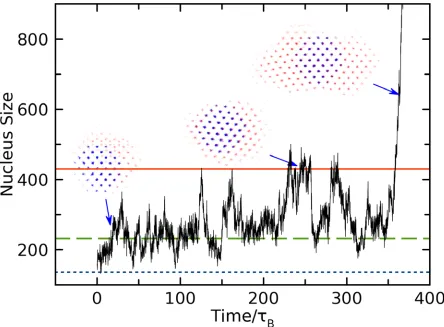
The critical nucleus size (𝑁𝑁∗) was computed by the following algorithm: as shown in Fig. 4, we
firstly plotted the embryo size (𝑁𝑁) versus time. According to the CNT, when the size of nucleus
reaches 𝑁𝑁∗, ∆𝐺𝐺 reaches a maximum: The nucleus has equal probability to either dissolve or further
grow. Therefore, the nucleus size will fluctuate around 𝑁𝑁∗ over a significant period of time,
reflected as a plateau in the 𝑁𝑁(𝑑𝑑) times series. To guarantee that the selected plateaus correspond
to the critical nucleus, we monitored the height and time width for each plateau. Occasionally,
there are sporadic plateaus driven by thermal fluctuations, but those are relatively low and narrow.
11
launched many independent simulations (up to 60) to generate significant statistics. A collection
of all plateaus is provided in Appendix A. For each plateau, we calculated its average height to
cancel out the thermal fluctuation. The critical nucleus size 𝑁𝑁∗, as well as the standard deviation
of the measurement, is then determined by averaging the heights of all the plateaus.
Fig. 4 shows a typical PEM simulation, where we show the embryo size versus time at 𝜌𝜌𝜎𝜎3 =
0.7525. ξ= 6 was applied in this case. There are several critical plateaus before the nucleus
irreversibly grows. The actual critical nucleus including all the atoms shows a clear anisotropic
[image:13.612.75.519.330.657.2]shape with obvious crystalline facets.
12
8 plateaus (see Appendix A for the collection). The three insets show the time-averaged shape of pre-critical, critical and post critical nuclei at the corresponding time (arrow). The blue dots indicate the embryo and red ones are particles attached to the embryo.
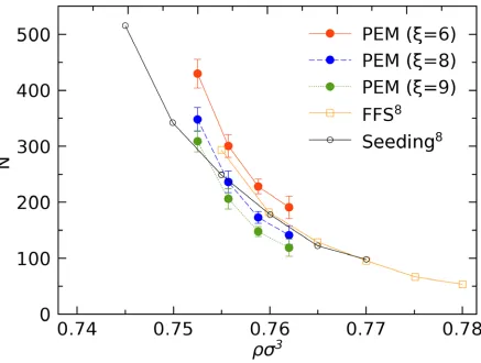
We considered at least 8 plateaus at every density. The averaged critical nucleus size 𝑁𝑁∗ and the
standard deviation are summarized in Table 2. A comparison between our result and ref. 8 is given
in Fig. 5. Overall, our results of ξ= 6 are in better agreement with those obtained by Forward Flux
Sampling (FFS)8 than those from the seeding method8. The deviation between PEM and the
seeding method may originate from the geometrical assumption of critical nucleus in seeding
method. Another comparison between PEM and the seeding method can be found in the
supplementary material of ref. 13. To make a comparison, both results from 𝜉𝜉 = 6, 8 and 9 are
13
Fig. 5: Critical nucleus size (𝑁𝑁∗) as a function of reduced (fluid) density (𝜌𝜌𝜎𝜎3). Both 𝜉𝜉= 6 (red solid line), 𝜉𝜉 = 8 (blue dash line) and ξ= 9 (green dot line) are considered. Previous results are given by either Forward Flux Sampling (FFS) or the seeding method from ref. 8, using 𝜉𝜉 = 9.
Table 2: Estimates for the nucleus size (𝑁𝑁∗) and its standard derivation (∆𝑁𝑁∗), attachment rate (𝑖𝑖+𝜏𝜏𝐵𝐵). 𝑁𝑁∗and Δ𝑁𝑁∗ are calculated in terms of 𝜉𝜉 = 6, 8 and 9, as shown explicitly.
𝜌𝜌𝜎𝜎3 𝑁𝑁∗±∆𝑁𝑁∗ (𝜉𝜉 = 6) 𝑁𝑁∗±∆𝑁𝑁∗ (𝜉𝜉= 8) 𝑁𝑁∗±∆𝑁𝑁∗ (𝜉𝜉 = 9) 𝑖𝑖+𝜏𝜏 𝐵𝐵
0.7525 429.76 ± 26.4 348.06 ± 21.1 308.89 ± 18.8 490.7
0.7557 300.67 ± 20.3 236.13 ± 19.3 206.09 ± 18.1 486.9
0.7588 228.30 ± 14.0 172.85 ± 10.6 147.65 ± 9.1 436.4
0.762 190.91 ± 19.9 141.31 ± 16.8 118.73 ± 15.3 437.8
[image:15.612.71.544.553.639.2]14
The attachment rate at the critical nucleus was calculated by the method first introduced by Auer
and Frenkel24. It considers the size change of the critical nucleus, based on the iso-configurational
ensemble25, which is given by the formula:
𝑖𝑖+ =〈|𝑁𝑁(𝑑𝑑)− 𝑁𝑁∗|2〉
2𝑑𝑑 (8)
To determine the attachment rate, we selected ta snapshot from PEM simulations whose nucleus
size is exactly 𝑁𝑁∗ as the initial configuration. We then performed 50 independent runs starting
from this configuration. Different trajectories were reached in these runs because of the random
noise introduced by reinitializing the random force term 𝑾𝑾(𝒕𝒕) in the Langevin equation for each
particle. (The springs are absent.)
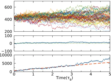
Fig. 6 shows a determination of attachment rates at 𝜌𝜌𝜎𝜎3 = 0.7525. From the upper panel we notice
that roughly half of the runs ended up melting back into the fluid, while the other half grew
irreversibly, as expected. Further confirmation is obtained by plotting the ensemble average
∆𝑁𝑁∗(𝑑𝑑) =𝑁𝑁(𝑑𝑑)− 𝑁𝑁∗. According to the CNT, 𝑑𝑑〈∆𝑁𝑁∗(𝑡𝑡)〉
𝑑𝑑𝑡𝑡 = 0 at 𝑁𝑁∗, which is clearly shown in Fig.
6. Therefore, we can measure the attachment rate by fitting the slope of |∆𝑁𝑁∗(𝑑𝑑)|2 to Equation 8.
15
Fig. 6: The upper panel shows the nucleus size versus time for the isoconfigurational ensemble including 50 runs. The middle panel shows the ensemble average of ∆𝑁𝑁∗(𝑑𝑑) =𝑁𝑁(𝑑𝑑)− 𝑁𝑁∗. The dot line (green) serves as a guide to the eye for the zero point. The bottom panel shows the ensemble average of |∆𝑁𝑁∗(𝑑𝑑)|2 = |𝑁𝑁(𝑑𝑑)− 𝑁𝑁∗|2. The dashed line (red) indicates the linear fitting to the range from 0.5𝜏𝜏𝐵𝐵 to 3𝜏𝜏𝐵𝐵 to derive the attachment rate. During 0.5𝜏𝜏𝐵𝐵 to 3𝜏𝜏𝐵𝐵, ∆𝑁𝑁∗(𝑑𝑑) remains to be almost zero.
6. Nucleation rate
The nucleation rate J is given by:
𝐽𝐽 =𝜅𝜅 exp (−Δ𝐺𝐺𝑘𝑘𝐵𝐵𝑇𝑇∗) (9)
where 𝜅𝜅 is a kinetic prefactor. Δ𝐺𝐺∗ depends on the driving force |Δ𝜇𝜇| and the critical nucleus size
16
Δ𝐺𝐺∗ =1
2𝑁𝑁∗|Δ𝜇𝜇| (10)
The explicit formula for the nucleation rate is26:
𝐽𝐽 =𝜌𝜌𝐿𝐿𝑖𝑖+�6𝜋𝜋𝑘𝑘|∆𝜇𝜇|
𝐵𝐵𝑇𝑇𝑁𝑁∗ exp�−
|∆𝜇𝜇|𝑁𝑁∗
2𝑘𝑘𝐵𝐵𝑇𝑇 � (11)
Nucleation rates were computed from Equation 11 and are summarized in Table 3. With nucleation
rates of the order of 10−15 or even smaller, it is not surprising that no nucleation events were
observed by brute-force simulation alone.
One should notice that the rate 𝐽𝐽 depends on 𝑁𝑁∗ exponentially, so a small uncertainty in 𝑁𝑁∗ will
result in a significant variation in 𝐽𝐽. Our calculation in terms of 𝜉𝜉= 6, 8 and 9 reconfirms this
statement. It is worth mentioning that PEM rigorously identifies the configuration of critical
nucleus. The error only enters in the identification of the number of solid-like particles. Further
[image:18.612.72.541.518.605.2]discussion about the order parameter can be found in ref. 27–29.
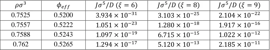
Table 3: Mapped volume fraction (𝜙𝜙𝑒𝑒𝑓𝑓𝑓𝑓, see below for its definition) and nucleation rate (𝐽𝐽𝜎𝜎5/𝐷𝐷) as a function of reduced density (𝜌𝜌𝜎𝜎3). Nucleation rate was calculated in the case of 𝜉𝜉= 6, 8 and
9.
𝜌𝜌𝜎𝜎3 𝜙𝜙
𝑒𝑒𝑓𝑓𝑓𝑓 𝐽𝐽𝜎𝜎5/𝐷𝐷 (𝜉𝜉= 6) 𝐽𝐽𝜎𝜎5/𝐷𝐷 (𝜉𝜉= 8) 𝐽𝐽𝜎𝜎5/𝐷𝐷 (𝜉𝜉 = 9)
0.7525 0.5200 3.934 × 10⁻³¹ 3.103 × 10⁻²⁵ 2.104 × 10⁻²² 0.7557 0.5222 1.051 × 10⁻²³ 1.280 × 10⁻¹⁸ 1.917 × 10⁻¹⁶ 0.7588 0.5243 1.097 × 10⁻¹⁹ 6.715 × 10⁻¹⁵ 1.022 × 10⁻¹² 0.762 0.5265 1.294 × 10⁻¹⁷ 5.120 × 10⁻¹³ 2.185 × 10⁻¹¹
7. Discussion
Computed nucleation rates are compared to other available estimates in Fig. 7. At a density of
17
(within error bar) to our PEM estimates. At the smaller density, PEM gives a slightly lower
nucleation rate than FFS from ref. 6. One should notice that the PEM calculations used the NVT
ensemble, while the US and FFS in ref. 4 operated in the NPT ensemble. As showed in Table 3,
the critical nucleus size at the density of 𝜌𝜌𝜎𝜎3 = 0.762 is 𝑁𝑁∗ = 190.91, while the total number of
system is 13500. When the nucleus reaches the critical size (𝑁𝑁∗), it is only 1% of the entire system.
In this case, the fluctuations that differentiate the NVT and NPT are virtually negligible5. In NVT
simulations, there is a feedback mechanism in that a growing crystalline nucleus has a higher
density and thus reduces the overall pressure, which prevents it from growing any further. Thus,
the NVT simulation actually evaluates the lower limit of the nucleation rates, as compared to the
NPT case. The influence of order parameter is explicitly shown in the Fig. 5, and we will discuss
it below. Besides, there is a recent paper30 which reveals that although FFS is not sensitive to order
parameter, the conventional FFS sometimes still underestimates the nucleation rate by several
orders of magnitude.
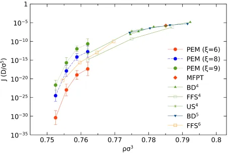
Furthermore, we also measured the nucleation rate at large densities where the nucleation can be
directly accessed by brute-force Brownian dynamics simulations. Mean-first passage time31 are
measured from 20 brute-force simulations. Computed nucleation rate is also shown in Fig. 7,
18
Fig. 7: The nucleation rate as a function of fluid density, in the case of 𝜉𝜉 = 6, 8 and 9. The results from previous work on WCA particles from ref. 4–6 are also included.
To translate the computed nucleation rates of WCA model with HS models, we map the density 𝜌𝜌
to the volume fraction 𝜙𝜙 by:
𝜙𝜙 =�𝜋𝜋6� 𝜌𝜌𝑑𝑑3 (12)
where 𝑑𝑑 is the effective diameter of WCA particles. Here we follow the same procedure as
described by Filion et al.4 to map the freezing density 𝜌𝜌𝑓𝑓𝜎𝜎3 ≃ 0.712 of WCA particles to the
freezing volume fraction 𝜙𝜙𝐹𝐹𝐻𝐻𝐻𝐻 of hard spheres. Even for the ideal HS model, there is some
uncertainty about the exact value of the freezing volume fraction, which is only accurately
determined within a range of 0.491 <𝜙𝜙𝐹𝐹𝐻𝐻𝐻𝐻 < 0.49423,32,33. In our study, we choose 𝜙𝜙𝐹𝐹𝐻𝐻𝐻𝐻≃ 0.492 ,
19
effective diameter 𝑑𝑑 ≃1.097𝜎𝜎. The mapped volume fraction is enclosed in Table 3. Note while
the uncertainty in 𝜙𝜙𝐹𝐹𝐻𝐻𝐻𝐻 appears to be quite small, it may result in a very large dispersion when
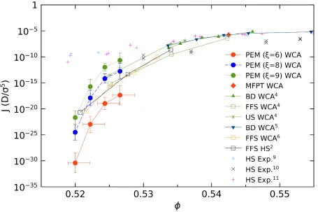
mapping the number density to the volume fraction. In Fig. 8, the nucleation rates are shown as a
function of volume fraction and compared to both experimental and other simulation results. The
horizontal error bar indicates the lower and upper limit for volume fractions. Given the logarithmic
nature of the plot, slight differences in the mapping result in large shifts of the nucleation rates.
Another crucial factor is the order parameter, as indicated in Fig. 5, Fig. 7 and Fig. 8. A small
change in 𝜉𝜉 can lead to a significant change in critical nucleus size (𝑁𝑁∗) and consequently, the
nucleation rate (𝐽𝐽). But the advantage of PEM is that it can get the exact configuration of the critical
nucleus, while the error is introduced in the counting of solid-like particles. Considering that the 𝐽𝐽
relies on 𝑁𝑁∗ exponentially, a small difference of 𝑁𝑁∗ can enhance a huge jump of 𝐽𝐽. Any method,
as long as it relies on CNT, suffers from this problem. On the other hand, the bond-orientational
order parameter is not the only representation of the solid particles within the nucleus. An
alternative option is the (𝑛𝑛,𝑣𝑣) parameter which incorporates a kinetic theory to the descriptor of
nucleus and can be used to describe the dynamics of sub-critical nucleus34,35.
Despite all these uncertainties, our WCA simulations are in clear agreement with previous
estimates2,4–6. However, all the computed nucleation rates, including current PEM results, deviate
from the experimental measurements9–11. As pointed out in ref. 4, this discrepancy is not related
to inaccuracies of the theoretical calculation but rather, reflects a true deficiency of HS and related
models to capture the physics of these experimental systems. Our calculations support this
20
Fig. 8: Nucleation rates as a function of mapped volume fraction, for 𝜉𝜉= 6 (red solid line), 𝜉𝜉 =
8 (blue dash line) and ξ = 9 (green dot line). Simulation resulting from WCA models4–6, hard spheres2 and experiments9–11 are included in the figure. The horizontal error bar when 𝜉𝜉= 8 and
9 is the same with the case when 𝜉𝜉= 6.
8. Conclusions
We have measured the chemical potential differences between undercooled WCA fluids and solids
by Gibbs-Helmholtz integration. We implemented the persistent-embryo method (PEM) to
evaluate the nucleation rates in the density of 𝜌𝜌𝜎𝜎3 = 0.7525, 0.7557, 0.7588, 0.762. The rates
given by PEM are consistent with the ones available from umbrella sampling (US) and forward
flux sampling (FFS). Our method-PEM is an efficient method to evaluate nucleation rates and
provides a unique characterization of not only the critical, but the dynamics of the pre-critical and
21
hard spheres. Our results provide more evidence that the discrepancy between simulation and
experiments will require more sophisticated models.
Conflicts of interest
There are no conflicts to declare.
Acknowledgements
Shang Ren would like to thank Xun Zha for help on HOOMD-blue. Work at Ames Laboratory was supported by the US Department of Energy, Basic Energy Sciences, Materials Science and Engineering Division, under Contract No. DE-AC02-07CH11358, including a grant of computer time at the National Energy Research Supercomputing Center (NERSC) in Berkeley, CA. K.M.H. acknowledges support from USTC Qian-Ren B (1000-Talents Program B) fund. The Laboratory Directed Research and Development (LDRD) program of Ames Laboratory supported the use of GPU-accelerated computing.
Reference
1 Debenedetti, Metastable liquids: concepts and principles, Princeton University Press, 1996.
2 L. Filion, M. Hermes, R. Ni and M. Dijkstra, J. Chem. Phys., 2010, 133, 244115.
3 S. Auer and D. Frenkel, Nature, 2001, 409, 1020–1023.
4 L. Filion, R. Ni, D. Frenkel and M. Dijkstra, J. Chem. Phys., 2011, 134, 134901.
5 T. Kawasaki and H. Tanaka, Proc. Natl. Acad. Sci., 2010, 107, 14036–14041.
6 D. Richard and T. Speck, J. Chem. Phys., 2018, 148, 124110.
7 J. R. Espinosa, C. Vega, C. Valeriani and E. Sanz, J. Chem. Phys., 2016, 144, 211801– 211922.
8 D. Richard and T. Speck, J. Chem. Phys., 2018, 148, 224102–124110.
9 K. Schätzel and B. J. Ackerson, Phys. Rev. E, 1993, 48, 3766–3777.
10 J. L. Harland and W. van Megen, Phys. Rev. E, 1997, 55, 3054–3067.
11 C. Sinn, A. Heymann, A. Stipp and T. Palberg, in Progr. Colloid Polym. Sci., Springer Berlin Heidelberg, Berlin, Heidelberg, 2001, vol. 118, pp. 266–275.
22
13 Y. Sun, H. Song, F. Zhang, L. Yang, Z. Ye, M. I. Mendelev, C. Z. Wang and K. M. Ho, Phys. Rev. Lett., 2018, 120, 085703.
14 J. D. Weeks, D. Chandler and H. C. Andersen, J. Chem. Phys., 1971, 54, 5237.
15 W. M. Brown, P. Wang, S. J. Plimpton and A. N. Tharrington, Comput. Phys. Commun., 2011, 182, 898–911.
16 W. M. Brown, A. Kohlmeyer, S. J. Plimpton and A. N. Tharrington, Comput. Phys. Commun., 2012, 183, 449–459.
17 W. M. Michael Brown and M. Yamada, Comput. Phys. Commun., 2013, 184, 2785–2793.
18 J. A. Anderson, C. D. Lorenz and A. Travesset, J. Comput. Phys., 2008, 227, 5342–5359.
19 J. Glaser, T. D. Nguyen, J. A. Anderson, P. Lui, F. Spiga, J. A. Millan, D. C. Morse and S. C. Glotzer, Comput. Phys. Commun., 2015, 192, 97–107.
20 P. J. Steinhardt, D. R. Nelson and M. Ronchetti, Phys. Rev. B, 1983, 28, 784–805.
21 P. Rein ten Wolde, M. J. Ruiz‐Montero and D. Frenkel, J. Chem. Phys., 1996, 104, 9932– 9947.
22 H. J. C. Berendsen, J. P. M. Postma, W. F. Van Gunsteren, A. Dinola and J. R. Haak, J. Chem. Phys., 1984, 81, 3684–3690.
23 D. Frenkel and S. Berend, Understanding molecular simulation: from algorithms to applications, Elsevier Science, San Diego, CA, 2001.
24 S. Auer and D. Frenkel, J. Chem. Phys., 2004, 120, 3015–3029.
25 A. Widmer-Cooper, P. Harrowell and H. Fynewever, Phys. Rev. Lett., 2004, 93, 135701.
26 K. F. Kelton and A. L. Greer, Nucleation in Condensed Matter: Applications in Materials and Biology, Elsevier, Amsterdam, 2010.
27 A. Haji-Akbari and P. G. Debenedetti, Proc. Natl. Acad. Sci., 2015, 112, 10582–10588.
28 H. Jiang, A. Haji-Akbari, P. G. Debenedetti and A. Z. Panagiotopoulos, J. Chem. Phys., 2018, 148, 44505.
29 N. E. R. Zimmermann, B. Vorselaars, J. R. Espinosa, D. Quigley, W. R. Smith, E. Sanz, C. Vega and B. Peters, J. Chem. Phys., 2018, 148, 222838.
30 A. Haji-Akbari, J. Chem. Phys., 2018, 149, 072303.
31 G. Chkonia, J. Wölk, R. Strey, J. Wedekind and D. Reguera, J. Chem. Phys., 2009, 130, 64505–154515.
32 R. L. Davidchack and B. B. Laird, J. Chem. Phys., 1998, 108, 9452–9462.
33 W. G. Hoover and F. H. Ree, J. Chem. Phys., 1968, 49, 3609–3617.
34 M. J. Uline, K. Torabi and D. S. Corti, J. Chem. Phys., 2010, 133, 174511.
23
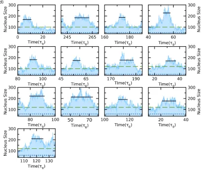
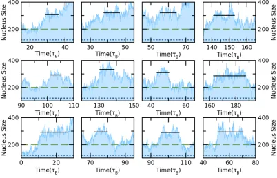
Appendix A: Collection of plateaus
25
Fig. A1: The plateaus to determine the critical nucleus size in different reduced densities (𝜌𝜌𝜎𝜎3): (a) 0.7525, (b) 0.7557, (c) 0.7588, (d) 0.762. During the PEM simulation, different 𝑁𝑁0, which is the size of embryo, and 𝑁𝑁𝑠𝑠𝑠𝑠, which is the threshold where the spin is removed, were applied and indicated by red dot line and green dash line, respectively. The black solid line shows the averaged height of each plateau.
Appendix B: The crystalline and geometrical structure of the embryo
To investigate the effect of geometry of embryo, we launched 36 independent PEM simulations in
the condition that the embryo is cubic, and 12 plateaus were collected among them. By the same
procedure, we find that the critical nucleus size (𝑁𝑁∗) for 𝜌𝜌𝜎𝜎3 = 0.7525 is 303.44 ± 15.4, while
in the spherical embryo case the 𝑁𝑁∗ = 300.67 ± 20.3. The two ranges have huge overlaps which
indicts that the geometry of embryo is not a critical issue in the PEM. A collection of plateaus is
26
Fig. A2: The plateaus to determine the critical nucleus size in the case of cubic embryo. The (reduced) density is 𝜌𝜌𝜎𝜎3 = 0.7557. During the PEM simulation, different 𝑁𝑁0, which is the size of embryo, and 𝑁𝑁𝑠𝑠𝑠𝑠, which is the threshold where the spin is removed, were applied and indicated by red dot line and green dash line, respectively. The black solid line shows the averaged height of each plateau.
Besides the geometry, another crucial factor is the structure of embryo, e.g. how does a BCC
embryo work in the PEM? This question has been discussed by Auer and Frenkel3, in the year of
2001. It is claimed that the BCC and icosahedral do not play a role in the nucleation process of HS
system. To test this, we launched 12 independent runs to justify the effect of BCC. The result
shows that the BCC embryo cannot grow while in the same time period the FCC embryo can lead
the crystallization, as shown in Fig. A3. Therefore, the BCC is not dominant if the nucleus is
27
[image:29.612.101.520.95.416.2]