Bifurcation and chaos of a particle motion system with holonomic constraint

Eng. Math. Lett. 2019, 2019:3 https://doi.org/10.28919/eml/3974 ISSN: 2049-9337

BIFURCATION AND CHAOS OF A PARTICLE MOTION SYSTEM WITH HOLONOMIC CONSTRAINT

NING CUI1∗, JUNHONG LI1,2

1_{Department of Mathematics and Sciences, Hebei Institute of Architecture and Civil Engineering, Zhangjiakou,}

Hebei 075000, China

2_{School of Mathematics and Statistics, Beijing Institute of Technology, Beijing, 100081,China}

Copyright c2019 the authors. This is an open access article distributed under the Creative Commons Attribution License, which permits

unrestricted use, distribution, and reproduction in any medium, provided the original work is properly cited.

Abstract. This paper investigates a holonomic constrained system of a particle moving on a horizontal smooth

plane. The equilibrium points, bifurcations and chaotic attractors of the system are analyzed. It shows that the

rich dynamic behaviors of the particle motion system, including the degenerate Hopf bifurcations at multiple

equilibrium points, the chaotic behaviors of the particle motion. The numerical simulations are carried out to

verify theoretical analyses and to exhibit the rich chaotic behaviors.

Keywords:bifurcation; particle motion; chaotic attractor.

2010 AMS Subject Classification:70K50, 34C23.

1.

Some research shows that the the particle motion becomes complex because of the existence

of external force, such as shear force [1] and creep force [2]. Junhong and his cooperators

studied a particle motion under external force and investigated the influences of two nonlinear

∗_{Corresponding author}

E-mail address: cnmath80@163.com

Received November 30, 2018

nonholonomic constraints on the particle motion [3]. In this paper, we will discuss the particle

motion system of Ref. [3] with holonomic constraint

x2+y2=M2(M>0).

By applying Lagrange’s method, the equations of holonomic system can be obtained as

fol-lows

(1)

  

¨

x=ax−bx2−cx₁y+2λx,

¨

y=ay−by2−cxy1+2λy,

Here λ is Lagrange’s multiplier. Differentiate the holonomic constraint equation twice with

respect to time and obtain ˙x2+xx¨+y˙2+yy¨=0, thenλ=−x

2

1+y21+aM2−bx3−by3−cx1xy−cxyy1

2M2 . Thus, the equations of motion of the constrained system become

(2)

              

˙ x=x₁,

˙

x₁=−bx₁2−cx₂x₃+ax₁−P₁(x,x₁,y,y₁), ˙

y=y₁, ˙

y₁=−bx₃2−cx₁x₄+ax₃−P₂(x,x₁,y,y₁). where

P1(x,x1,y,y1) =

x1((−bx12−cx2x3+ax1)x1+(−bx32−cx1x4+ax3)x3+x22+x42)

M2 ,

P₂(x,x₁,y,y₁) =x3((−bx1 2_−cx

2x3+ax1)x1+(−bx32−cx1x4+ax3)x3+x22+x42)

M2 .

The stability of equilibrium points, Hopf bifurcation and chaos of the constrained system are

investigated as follows.

2.

By computations, we can obtain the equilibrium points as follows

E0= (0,0,0,0),E1= (0,0,M,0),E2= (0,0,−M,0),E3= (0,0,a_b,0), E₄= (M,0,0,0),E₅= (−M,0,0,0),E₆= (a_b,0,0,0),E₇= (a_b,0,a_b,0), E8= (−√M₂,0,−√M₂,0),E9= (√M₂,0,√M₂,0).

The characteristic equations at equilibrium points are obtained as follows

fE0(λ) =λ 4_−a

λ2−λ3+aλ,

f_E1(λ) =λ4+ (cM−1)λ3+ (−bM−cM)λ2+bMλ,

fE3(λ) =λ

4₊(ca−b)λ3

b −

a(b+c)λ2 b +aλ,

f_E4(λ) =λ4+ (cM−1)λ3+ (−2bM−cM+2a)λ2+ −2M2bc+2Mac+2bM−2aλ +2cM(bM−a),

f_E5(λ) =λ4+ (−cM−1)λ3+ (2bM+cM+2a)λ2+ −2M2bc−2Mac−2bM−2aλ +2cM(bM+a),

f_E6(λ) =λ4+(ca−b)λ

3

b +

a(b2M2−M2bc−a2)λ2 b2_M2 +

a(b2M2−a2)(ca−b)λ b3_M2 −

ca2(b2M2−a2)

b3_M2 ,

fE7(λ) =λ

4₋(ca+b)λ3

b −

a(3b2M2−M2bc−7a2)λ2 b2_M2 +

a(3b2M2−7a2)(ca+b)λ b3_M2 −

ca2(3b2M2−7a2)

b3_M2 .

fE8(λ) =λ

4_{+ (cM}√_2/2−1)λ3_{+ (−cM}√_2/2−bM√_2/4+a)λ2_{+ (−M}2_bc/2

+M√2ac/2+bM√2/4−a)λ+M2bc/2−1/2M √

2ac,

fE9(λ) =λ

4_{+ (−cM}√_2/2−1)

λ3+ (cM √

2/2+bM√2/4+a)λ2+ (−M2bc/2 −M√2ac/2−bM√2/4−a)λ+M2bc/2+M

√

2ac/2.

From the expression of f_E6(λ), we can obtain the eigenvalues are± √

ab2_M2_−a3

bM i, 1,

ac

b, where a

Mb <1. In this case, the system occurs Hopf bifurcation at the equilibriumE6. ForE6, let        

x−a_b

x1 y y1         =            

0 √ bM

ab2_M2_−a3 0 0

1 0 0 0

0 0 0 ca_ba+b

0 0 1 1

                    u₁ u2 u₃ u4         .

Then, the system (2) becomes

(3)                  ˙ u₁=−

√

ab2_M2_−a3

bM u2+G1(u1,u2,u3,u4), ˙

u2=

√

ab2_M2_−a3

bM u1+G2(u1,u2,u3,u4), ˙

u₃=−cMu₃+G₃(u₁,u₂,u₃,u₄), ˙

u₄=u₄+U₄(u₁,u₂,u₃,u₄), where

G₁(u₁,u₂,u₃,u₄) =− b3M2u22 M2_ab2_−a3−

cu1(ac+b)u4 ba +

abMu2

√

M2_ab2_−a3−

bu2 M√M2_ab2_−a3(

bMu2

√

M2_ab2_−a3

×(− b3M2u22 M2_ab2_−a3−

cu1(ac+b)u4 ba +

abMu2

√

M2_ab2_−a3) +

(ac+b)u4 ba (−

(ac+b)2u42 ba2 −

cbMu_√ 2(u3+u4) M2_ab2_−a3 +(ac+b)u4

b +u 2

1+ (u3+u4)2) +

√

G₂(u₁,u₂,u₃,u₄) =0,

G₃(u₁,u₂,u₃,u₄) =cMu₃−(ac+b)2u42 ba2 −

cbMu_√ 2(u3+u4) M2_ab2_−a3 +

(ac+b)u4 b −

(ac+b)u4 abM2 (

bMu2

√

M2_ab2_−a3

×(− b3M2u22 M2_ab2_−a3−

cu1(ac+b)u4 ba +

abMu2

√

M2_ab2_−a3) +

(ac+b)u4 ba (−

(ac+b)2u42 ba2 −

cbMu_√ 2(u3+u4) M2_ab2_−a3 +(ac+b)u4

b ) +u21+ (u3+u4)2), G4(u1,u2,u3,u4) =0.

Furthermore,

g11= 1₄(− 2b 3_M2

M2_ab2_−a3),g02= 1 4(

2b3_M2 M2_ab2_−a3),

g₂₀= 1₄( 2b3M2

M2_ab2_−a3), g21 = 1 8(

6b3Ma

(M2_ab2_−a3₎3/2 +

2b

M√M2_ab2_−a3i),

thus

Rec1(0) =Re(√_M2Mbi_ab2_−a3(g20g11−2|g11| 2₋1

3|g02| 2_{) +}1

2g21) = 1 8

b2

M2_ab2_−a3 >0.

Based on the above analysis and the theorem in [4], we can obtain the the conclusion as

follows.

Theorem 1.The system (2) undergoes degenerate Hopf bifurcations atE₆and the bifurcating periodic solution is unstable.

According to Routh-Hurwitz criteria, E₀, E₁, E₅, E₇ and E₉ are unstable points. For the other equilibria, we can obtain the same conclusions using the method in [4] when the Hopf

bifurcations occur.

3.

The above results show that the particle motion system has complex dynamic behaviors. In

this section, we give some simulations to study the particle motion and select the parameters

a=5, c=0.001,b=1, and initial values(x₀,x₁₀,y₀,y₁₀) = (0.1,0.001,0.1,0.1). In this case, the system (2) has ten equilibrium points. Table.1 indicates the eigenvalues of corresponding

Jacobian matrix and the equilibria type and shows the unstable manifold and stable manifold at

the equilibrium points of the particle motion system whenM=0.2.

In chaos theory, the equilibrium points of the system are of great importance to understand

its nonlinear dynamics [5]. It has been long supposed that the existence of chaotic behaviour

[6] and the interconversion of the stable manifolds and the unstable manifolds which can cause

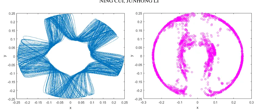
complicated dynamics in the system (2)[7-8]. The Lyapunov exponents are 0, -0.2 -0.3 and

0.6 using the method in [7], thus the system (2) is chaotic. Fig 1. shows the particle motion

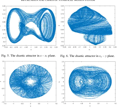
trajectory and the chaotic attractor of the system. The poincare maps and chaotic attractors in

x−y plane andx1−y1 plane are given in Fig. 1-6. If the constrained parameter M=1, the particlemotion system also occur chaotic phenomena. Fig. 7-8 show the chaotic ayyractor in

x−yplane andx−x1plane.

TABLE1. The eigenvalues of corresponding Jacobian matrix and the equilibria type.

equilibrium points eigenvalues of Jacobian matrix equilibria type

(0,0,0,0) 0, 1,2.2361, -2.2361 unstable equilibrium point

(0,0,0.2,0) 0, 1, 0.44731, -0.44731 unstable equilibrium point

(0,0,-0.2,0) 0, 1,±0.44721i Hopf bifurcation

(0,0,5,0) 0, 1, -2.23857, 2.23357 unstable equilibrium point

(0.2,0,0,0) 1, 0.0024, 0.0612±3.9763i unstable equilibrium point

(-0.2,0,0,0) 1, 0.0026, -0.0637±3.22442i unstable equilibrium point

(5,0,0,0) 1, -0.005, 55.8569, -55.8569 unstable equilibrium point

(5,0, 5,0) 1, 59.069, -0.01, -52.819 unstable equilibrium point

(−0√.2

2 ,0,-0.2

√

2,0) 1, 0.0001,±2.25182i Hopf bifurcation (0√.2

2,0, 0.2

√

Fig. 1. The chaotic attractor inx−yplane. Fig. 2. The poincare map inx−yplane.

Fig. 3. The chaotic attractor inx₁−y₁plane. Fig. 4. The poincare map inx1−y1plane.

4.

The results show that the rich dynamic behaviors of the particle motion system, including

Hopf bifurcations, interconversion of the stable manifolds and the unstable manifolds at

multi-ple equilibrium points and chaotic attractors. Thus, the particle motion trajectory has commulti-plex

dynamic behaviors under the holonomic constraint.

Acknowledgements

Project supported by the Youth Science Foundations of Education Department of Hebei Province

(No. QN2016265), Hebei Special Foundation “333 talent project”(No. A2016001123), and

Sci-entific Research Funds of Hebei Institute of Architecture and Civil Engineering (Nos. 2016XJJQN03,

Fig. 5. The chaotic attractor inx−x1plane. Fig. 6. The chaotic attractor inx1−yplane.

Fig. 7. The chaotic attractor inx−yplane. Fig. 8. The chaotic attractor inx−x1plane.

Conflict of Interests

The authors declare that there is no conflict of interests.

REFERENCES

[1] D. J. Pine, J.P Gollub, J. F. Brady, A. M. Leshansky, Chaos and threshold for irreversibility in sheared

suspensions, Nature, 438 (2005), 997-1000.

[2] L. Enkeleida, M. V. Petia, Periodic and chaotic orbits of plane-confined micro-rotors in creeping flows, J

Nonlinear Sci., 25 (2015), 1111-1123.

[3] J. Li, H. Wu, F. Mei, Dynamic analysis for the hyperchaotic system with nonholonomic constraints, Nonlinear

Dynam., 90 (4) (2017), 2257-2269.

[4] B. Hassard, N. Kazarino, Y. Wan, Theory and Appli-cation of Hopf Bifurcation, Cambridge University Press,

Cambridge, (1982).

[6] P. Gaspard, M. E. Briggs, M. K. Francis, J.V. Sengers, R.W. Gammon, J.R. Dorfman, R.V. Calabrese,

Exper-imental evidence for microscopic chaos, Nature, 394(6696) (1998), 865-868.

[7] S. Cang, A. Wu, Z. Wang, Z. Chen. On a 3-D generalized Hamiltonian model with conservative and

dissipa-tive chaotic flows, Chaos Soliton. Fract., 99 (2017), 45-51.

[8] F. Li, C. Yao, The infnite-scroll attractor and energy transition in chaotic circuit, Nonlinear Dynam., 84

(2016),2305-2315.

[9] A Wolf, JB Swift, HL Swinney, JA Vastano, Determining Lyapunov exponents from a time series, Physica