in the population sciences published by the Max Planck Institute for Demographic Research Konrad-Zuse Str. 1, D-18057 Rostock · GERMANY www.demographic-research.org
DEMOGRAPHIC RESEARCH
VOLUME 15, ARTICLE 21, PAGES 561-590
PUBLISHED 15 DECEMBER 2006
http://www.demographic-research.org/Volumes/Vol15/21/ DOI: 10.4054/DemRes.2006.15.21
Research Article
Mortality tempo-adjustment:
An empirical application
Marc Luy
© 2006 Luy
This open-access work is published under the terms of the Creative Commons Attribution NonCommercial License 2.0 Germany, which permits use, reproduction & distribution in any medium for non-commercial purposes, provided the original author(s) and source are given credit.
2 Why life expectancy differences between western and eastern Germany call for tempo-adjustment
564
3 Trends in tempo-adjusted life expectancy in western and eastern Germany
570
4 Discussion 574
5 Acknowledgements 579
References 580
Mortality tempo-adjustment: An empirical application
Marc Luy 1
Abstract
The number of scholars following the tempo approach in fertility continues to grow, whereas tempo-adjustment in mortality generally still is rejected. This rejection is irra-tional in principle, as the basic idea behind the tempo approach is independent of the kind of demographic event. Providing the first empirical application to a substantial problem, this paper shows that mortality tempo-adjustment can paint a different picture of current mortality conditions compared to conventional life expectancy. An applica-tion of the Bongaarts and Feeney method to the analysis of mortality differences be-tween western and eastern Germany shows that the eastern German disadvantages still are considerably higher and that the mortality gap between the two entities began to narrow some years later than trends in conventional life expectancy suggest. Thus, the picture drawn by tempo-adjusted life expectancy fits the expected trends of changing mortality and also the self-reported health conditions of eastern and western Germans better than that painted by conventional life expectancy.
1. Introduction
One of the main goals of quantitative demography is the derivation of period measures with a clear and distinct meaning to analyze demographic developments in time as well as current demographic conditions in different populations. Since more than a century demographers have been assuming to know how to provide correct calculations and interpretations of period measures, such as the total fertility rate (TFR) or life
expec-tancy at birth (e0). Both are summary measures and have the purpose to represent
cur-rent fertility and mortality conditions respectively, standardized for the given age com-position of populations driving the number of observed events and thus the values of crude rates.
In a series of papers, Bongaarts and Feeney (1998, 2002, 2003, 2006) recently have claimed that summary measures such as these should not only be standardized for age but also for tempo effects that arise whenever demographic conditions are chang-ing. In their most recent paper, Bongaarts and Feeney (2006: 116) define a tempo dis-tortion as an “inflation or deflation of a period quantum or tempo indicator of a life-cycle event, such as birth, marriage, or death, resulting from a rise or fall in the mean age at which the event occurs”. Introducing the idea with corresponding formulae for tempo-adjustment, Bongaarts and Feeney stirred the world of demographers and di-vided their community into tempo supporters and tempo opponents. Despite existing critics (e.g., Van Imhoff and Keilman, 2000; Kim and Schoen, 2000; Van Imhoff, 2001; Smallwood, 2002; Schoen, 2004; Keilman, 2006), the number of scholars following the tempo approach in fertility continues to grow (see e.g., Lesthaeghe and Willems, 1999; Kohler and Philipov, 2001; Philipov and Kohler, 2001; Zeng Yi and Land, 2001, 2002; Goldstein et al., 2003; Sobotka, 2003, 2004a, 2004b; Winkler-Dworak and Engelhardt,
2004).2 However, Bongaarts and Feeney’s successive work on mortality tempo effects
still is generally rejected (see Guillot, 2003b, 2006; Le Bras, 2005; Wachter, 2005; Wilmoth, 2005; Rodríguez, 2006).
The rejection is irrational in principle, as the basic idea behind the tempo approach
is independent of the kind of demographic event.3 The idea of adjusting period life
expectancy for tempo effects is as follows. When deaths are postponed to increasingly later ages, the number of deaths occurring in a given period is thinning out. For exam-ple, if every death in a given year were to be postponed by six months, there would be only half as many deaths observed in that year as one would have expected if there had been no postponement at all. Because death rates would decline at all ages, life expec-tancy would increase by a larger amount, many times the half a year that was actually added to the length of life in that period. Tempo-adjustment produces a period measure of longevity that changes only by the amount of lifetime by which deaths were
post-poned, and as such is a potentially useful tool for demographers.4 It has already been
shown that in a given situation of mortality decline, i.e. the mean age at death increases, life expectancy calculated from age-specific death rates during the period of changing mortality conditions is higher than life expectancy calculated from age-specific death rates under stationary mortality conditions at the end of this transition (Bongaarts and Feeney, 2002, 2006; Feeney, 2003; Horiuchi, 2005). An illuminating paper about the consequences of such biases on the interpretation of period data was written by Vaupel (2002), who called for a distinction between “life expectancy at current rates” and “life
expectancy at current conditions”.5
It seems that tempo effects impact current period measures for mortality signifi-cantly, as they do with fertility measures. In the actual discussion on mortality tempo, this aspect is given no consideration: the published papers solely deal with theoretical and technical questions, while empirical applications are used exclusively to compare different measures of period mortality conditions and to demonstrate their properties against the background of historical mortality trends (besides the Bongaarts and Feeney papers mentioned above, see e.g. Vaupel, 2002, 2005; Feeney, 2003, 2006; Guillot, 2003b, 2006; Bongaarts, 2005; Le Bras, 2005; Wachter, 2005; Wilmoth, 2005; Gold-stein, 2006; Rodríguez, 2006). Empirical applications to a substantive problem of mor-tality differentials are, however, missing so far. An interesting aspect – although not explicitly mentioned by the authors – of the initial mortality tempo paper of Bongaarts and Feeney (2002) is that the variance in life expectancy between the US, Sweden, Japan, and France decreases from 3.4 years according to conventional life expectancy to only 1.7 years according to tempo-adjusted life expectancy. Applying the Bongaarts
period rates are used to derive any other demographic measures, then these measures are affected by tempo distortions. It does not matter whether they contain a quantum component or not, as is the case in period life expectancy.
4 The author thanks an anonymous referee of this paper for his or her suggestion to include this example in order to describe the basic idea of mortality tempo-adjustment.
and Feeney method to mortality differences between eastern and western Germany, I will show that adjusting period life expectancy for tempo effects paints a different pic-ture of mortality trends and of differences between these two regions than conventional tempo-unadjusted calculations. I will conclude that the results of tempo-adjusted life expectancy provides a better fit to the expected trends of changing mortality, and also to self-reported health conditions of eastern and western Germans.
2. Why life expectancy differences between western and eastern
Germany call for tempo-adjustment
The demographic changes and developments in eastern and western Germany are gen-erally seen to present a unique opportunity to understand the interaction between socie-tal, social, and economic conditions on the one hand, and population processes on the other. The German experience thus is used to understand the reasons behind recent mortality changes. The two pre-war German regions were characterized by a demo-graphic composition and behavior that was almost identical until 1945, followed how-ever by 45 years under different political and socio-economic structures and resulting in demographic developments that were entirely different (Dinkel, 1992, 1994, 1999; Gjonça et al., 2000). With unification in 1990, East Germany adopted the western so-cietal and economic system, causing sudden changes in all of its demographic proc-esses. These conditions – leading some scholars to describe the eastern German popula-tion as a kind of “natural experiment” (Dinkel, 1999; Vaupel et al., 2003) – generated a large number of studies on the changes in eastern German demography. Of central interest in the field of mortality research has been the rapid convergence of life expec-tancy since 1990 following roughly two decades of continuous divergence. The former widening and the subsequent closing in the life expectancy gap between western and eastern Germany were mainly caused by the age groups 60-80, leading to the central message that “it’s never too late” to increase one’s length of life (Vaupel et al., 2003).
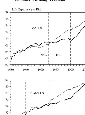
Figure 1 shows the trends in period life expectancy at birth e0, using standard life
table techniques for western and eastern German women and men for each single cal-endar year from 1950 to 2004. The life table calculations are based on official popula-tion statistics, i.e. data for the living populapopula-tion and deaths for each calendar year and
single age groups (for a more detailed description of these data, see Luy, 2004a).6
Figure 1: Trends in conventional life expectancy at birth for western and eastern Germany, 1950-2004
62 64 66 68 70 72 74 76 78
1950 1960 1970 1980 1990 2000
West East
Life Expectancy at Birth
MALES
66 68 70 72 74 76 78 80 82
1950 1960 1970 1980 1990 2000
Calendar Year FEMALES
Phase I Phase II Phase III IV V
Regarding mortality differences between western and eastern Germany, the time span presented can be subdivided into five central phases:
• The first phase, from 1950 to roughly 1960, is characterized by irregular
fluc-tuations, with several years of mortality crossing over. These trends corre-spond with the waves of influenza that swept East and West Germany in dif-ferent years (Luy, 2004a). No mortality differences can be detected between the two Germanys, neither for men nor for women.
• In the second phase, roughly covering the period 1960 to 1975, the
develop-ments in life expectancy in West and East Germany assumed more regularity, with mortality slightly higher among East German women and significantly lower among East German men. The differences in favor of East German males rose until the first half of the 1970s and reached a maximum of roughly one year in life expectancy at birth. However, the disadvantage of West Ger-man men arose mainly from different definitions of live birth in East and West Germany, thus causing lower infant mortality rates in the former GDR on
sta-tistical grounds.7 An analysis of age-specific differences between West and
East German mortality shows that the higher life expectancy among East Ger-man men mainly (but not only) resulted from statistically lower infant mortal-ity (Luy, 2004a).
• The third phase, starting in the middle of the 1970s, is characterized by the
continuous divergence for both sexes in the development of mortality condi-tions in favor of West Germany. This development corresponds to the general divergence in mortality trends between all western and eastern European coun-tries (e.g. Caselli and Egidi, 1980; Bourgois-Pichat, 1985; Bobak and Marmot, 1996a, 1996b; Hertzman et al., 1996; Meslé and Hertrich, 1997; Vallin and Meslé, 2001; Meslé and Vallin, 2002). Figure 1 shows that the widening of the life expectancy gap was caused by the fact that East German life expectancy at birth increased at a lower pace for both sexes, whereas life expectancy in West Germany rose more rapidly (Höhn and Pollard, 1991; Scholz, 1996; Gjonça et al., 2000; Nolte et al. 2000a). The differences peaked in 1988 for women (al-most 3 years) and in 1990 for men (roughly 3.5 years).
• These peaks – virtually concurring with German unification – were followed by the continuous narrowing of the gap in west-east German mortality
differ-ences until the end of the 1990s, when the difference in e0 reached about 0.5
years for women and about 1.6 years for men. As can be seen in Figure 1, as the two Germanys entered this phase the differences in life expectancy trends between them started to reverse compared to the trends in the third phase. The convergence of mortality levels now observable is due to the fact that since the beginning of the 1990s life expectancy has been rising much faster in eastern Germany than in the west. Based on these observations, German demographers assumed that the west-east mortality gap will fully close during the first two
decades of the 21st century, as reflected in one of the most recent population
forecasts of the Statistical Office of Germany (Statistisches Bundesamt, 2003).
• However, around the year 2000, this trend changed again. The differences in
life expectancy between eastern and western German men now stagnate on a level around 1.5 years. Eastern German women, by contrast, seem to further approximate the western German level, however with a decline in the pace of approximation and with the difference now being around 0.25 years.
Figure 1 shows a striking decrease in life expectancy among eastern German men in 1990, a phenomenon described as the eastern German “mortality crisis” (Dorbritz and Gärtner, 1995; Riphan, 1999; Nolte et al., 2000a, 2000b) and as characteristic of a “demographic shock” in connection with the changes in eastern Germany resulting from unification (Eberstadt, 1994). However, long-term trends in life expectancy ques-tion the aptness of this descripques-tion and call for an explanaques-tion of the rapid closing of the gap. The decisive question is: Which factor or which factors are responsible for the trend reversal in mortality differences between western and eastern Germany, a trend reversal that has occurred within one or two years only? The factors discussed most in search of an answer are the same that are assumed to be responsible for the general mortality gap between western and eastern European countries (e.g. Bobak and Mar-mot, 1996a, 1996b; Hertzman et al., 1996; for the discussion on the mortality differ-ences between eastern and western Germany, see Luy, 2004a): East German working conditions, environmental conditions, the consequences of uranium mining and storage, the effects of the ongoing immigration of a more healthy foreign population to West Germany, selective internal east-west migration, psychological reactions to the political suppression, economic conditions, medical technology, lifestyles, and cardiovascular risk factors.
main cause(s) for the mortality differences between western and eastern Germany will be an important step forward in gaining a deeper understanding of general mortality differentials. A large and continuously increasing number of studies follow this path based on trends in life expectancy such as shown in Figure 1 (e.g. Chruscz, 1992; Dinkel, 1994, 1999; Schott et al., 1994; Becker and Boyle, 1997; Gjonça et al., 2000; Bucher, 2002; Nolte et al., 2002; Luy, 2004a, 2004b, 2005b; Mai, 2004). Although many researchers are working on this subject, the rapid approximation of life expec-tancy is still not explained in full.
However, following Bongaarts and Feeney’s tempo approach, we must conclude that period life expectancy based on annual age-specific death rates is an imperfect solution for the reflection of period mortality conditions. This is because death rates are biased downward with rising mean age at death (mortality decline) and they are biased upward when the mean age at death declines (mortality increase). Since different popu-lations experience changes in the mean age at death with different paces, tempo effects impact them differently. Phases of mortality decline and phases of mortality increase set in in eastern and western Germany in different years and with different pace, coinciding with observed trends in life expectancy differences between the two parts of Germany: during Phase 3, life expectancy increased continuously in West Germany, whereas it rose only slightly or remained constant in the east. During Phase 4, life expectancy rose more steeply in eastern Germany than in the west. We can assume that the sudden im-provements in eastern Germany after unification, for instance in economic conditions and medical technology, caused postponement of deaths in almost all age groups to an extent that was not possible in western Germany, where these conditions have already been on a high level. Similarly, for the years preceding unification we can expect that more deaths among western German women and men have been postponed as a conse-quence of increasing advantages in living conditions and medical standards. If these different trends are causing tempo distortions in the sense of Bongaarts and Feeney’s approach, then the studies on the causes of eastern German excess mortality are based on data leading to a distorted picture of mortality conditions in the two German regions and thus to the differences between them. In the final consequence, this may be the reason why the factor(s) mainly responsible for the impressive improvement of mortal-ity conditions in eastern Germany is (are) still undetected.
In the following, tempo-adjusted life expectancy, denoted by e0*(t), for western
Figure 2: Conventional life expectancy at birth e0(t) and smoothed
estimates e0(t)S (sixth degree polynomial), western and eastern Germany, 1950-2004 (no mortality under age 30)
(a) western Germany, Males
70 71 72 73 74 75 76 77 78 79
1950 1960 1970 1980 1990 2000 Calendar Year t
L if e E x p ect an cy _ e0(t) e0(t)S e0(t)
e0(t) S
(b) eastern Germany, Males
70 71 72 73 74 75 76 77
1950 1960 1970 1980 1990 2000 Calendar Year t
L if e E x p ect an cy _ e0(t) e0(t)S e0(t)
e0(t)S
(c) western Germany, Females
73 74 75 76 77 78 79 80 81 82 83
1950 1960 1970 1980 1990 2000 Calendar Year t
L if e E x p ect an cy _ e0(t) e0(t)S e0(t)
e0(t)S
(d) eastern Germany, Females
73 74 75 76 77 78 79 80 81 82 83
1950 1960 1970 1980 1990 2000 Calendar Year t
L if e E x p ect an cy _ e0(t) e0(t)S e0(t)
observed (i.e., e0(t) = e30(t) + 30). These functions form the base for the method used to
calculate tempo-adjusted life expectancy e0*(t) in eastern and western Germany. The
formula used for tempo-adjusted life expectancy is
− + =
dt (t) de b
(t) e (t) e
* 0 0
*
0 ln 1
1
,
with b denoting the “Gompertz parameter” estimated by fitting a Gompertz model to annual age-specific death rates. The methods of estimation and the calculations done for western and eastern Germany are provided in the Appendix.
3. Trends in tempo-adjusted life expectancy in western and eastern
Germany
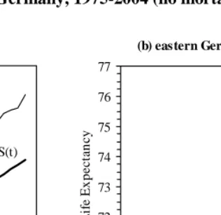
Figure 3 shows the trends in conventional and tempo-adjusted life expectancy at birth (no mortality under age 30 in both cases) from 1975 to 2004 for western and eastern German females and males. The graph for western German females (Figure 3c) is very similar to the figures for US and Japanese women presented by Bongaarts and Feeney (2002: 24). As can be seen in Figure 2(c), western German females represent the only of the four populations analyzed with an observed life expectancy at birth that has been increasing almost constantly since 1950. Thus, the tempo distortion S(t) (defined as the difference between conventional and tempo-adjusted life expectancy) is relatively con-stant among western German females during the observation period. Since improve-ments in life expectancy developed later (western and eastern German males) or at a changing pace (eastern German females) among the other three populations, tempo distortions must vary when compared to western German females. This is well reflected
by the results gained for e0*(t) and S(t), as can be seen in Figure 3.
Figure 3: Conventional life expectancy at birth e0(t) and estimated tempo-
adjusted life expectancy at birth e0*(t) with tempo distortion S(t),
western and eastern Germany, 1975-2004 (no mortality under age 30)
(a) western Germany, Males
70 71 72 73 74 75 76 77 78 79
1975 1980 1985 1990 1995 2000 2005 Calendar Year t
L if e E x p ect an cy __
e0(t)
e0*(t)
S(t)
(b) eastern Germany, Males
70 71 72 73 74 75 76 77
1975 1980 1985 1990 1995 2000 2005 Calendar Year t
L if e E x p ect an cy __
e0(t)
e0*(t)
S(t)
(c) western Germany, Females
75 76 77 78 79 80 81 82 83
1975 1980 1985 1990 1995 2000 2005 Calendar Year t
L if e E x p ect an cy __
e0(t)
e0*(t) S(t)
(d) eastern Germany, Females
75 76 77 78 79 80 81 82 83
1975 1980 1985 1990 1995 2000 2005 Calendar Year t
L if e E x p ect an cy __
e0(t)
e0*(t)
although at a lower pace than does conventional life expectancy. Among eastern Ger-man males, life expectancy remained constant or even declined slightly until the end of the 1980s and then started to rise at a higher pace than in any phase of life expectancy trends in western Germany (Figures 2a and 2b). Consequently, tempo-adjusted life
expectancy e0*(t) did not differ from conventional life expectancy until the beginning of
the 1990s and then began to increase at a considerably lower rate compared to e0(t). The
extent of tempo distortions in conventional life expectancy grew during the observed period among eastern German females, too. From Figure 2(d) we know that their life expectancy rose in the period preceding unification, although it did so at a lower pace than among their West German counterparts (see also Figure 1). As a result, tempo distortions, i.e. the difference between tempo-adjusted and conventional life expec-tancy, remained at an almost constant level between 1975 and 1990. However, the
dif-ference between e0(t) and e0*(t) started to increase at the end of the 1980s when
conven-tional life expectancy rose at a higher rate – a phenomenon similar to what has been observed among men in the eastern part of Germany (Figures 3b and 3d).
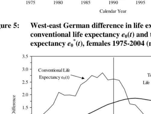
Figure 4: West-east German difference in life expectancy at birth for conventional life expectancy e0(t) and tempo-adjusted life
expectancy e0*(t), males 1975-2004 (no mortality under age 30)
-1.0 -0.5 0.0 0.5 1.0 1.5 2.0 2.5 3.0 3.5
1975 1980 1985 1990 1995 2000 2005
Calendar Year W es t-E as t-D iff er en ce __ Conventional Life Expectancy e0(t)
Tempo-Adjusted
Life Expectancy e0 *
(t)
Unification
Figure 5: West-east German difference in life expectancy at birth for conventional life expectancy e0(t) and tempo-adjusted life
expectancy e0*(t), females 1975-2004 (no mortality under age 30)
-1.0 -0.5 0.0 0.5 1.0 1.5 2.0 2.5 3.0 3.5
1975 1980 1985 1990 1995 2000 2005
Calendar Year W es t-E as t-D if fer en ce __ Conventional Life
Expectancy e0(t) Tempo-Adjusted
Life Expectancy e0*(t)
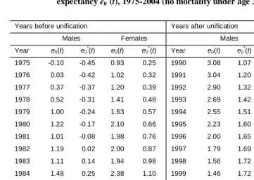
those in tempo-adjusted life expectancy are now even higher, with a difference of about 1.6 years. Only at the end of the 1990s did the trend in increasing differences in tempo-adjusted life expectancy lower in speed, pointing to slow convergence solely in the last years of the observation period.
The results for the west-east German differences among females are similar to those just described for males. Until unification, the advantage in mortality conditions of West German females is lower when tempo-adjusted life expectancy is used instead of conventional life expectancy. Whereas the difference in conventional life expectancy increased to 2.85 years in 1988, those in tempo-adjusted life expectancy did never ex-ceed 1.9 years. Similar to the situation among men, the differences in tempo-adjusted life expectancy between western and eastern German females did not decline with uni-fication parallel to conventional life expectancy but instead rose until the mid 1990s. The trends in conventional and tempo-adjusted life expectancy crossed over between 1992 and 1993. From then on, the mortality advantage of western German females measured with tempo-adjusted life expectancy is higher when compared to the results based on tempo-unadjusted values. Although a decreasing trend in mortality differences between western and eastern German females is also evident with tempo-adjusted life expectancy since the mid 1990s, the remaining differences in favor of western German women are still considerably higher. While the disadvantage of eastern German women decreased to 0.28 years in the year 2004 according to conventional life expectancy, the tempo-adjusted difference still shows 1.1 years.
4. Discussion
Table 1: West-east German difference in life expectancy at birth according to conventional life expectancy e0(t) and tempo-adjusted life
expectancy e0*(t), 1975-2004 (no mortality under age 30)
Years before unification Years after unification
Males Females Males Females
Year e0(t) e0
*
(t) e0(t) e0
*
(t) Year e0(t) e0
*
(t) e0(t) e0
*
(t)
1975 -0.10 -0.45 0.93 0.25 1990 3.08 1.07 2.61 1.69
1976 0.03 -0.42 1.02 0.32 1991 3.04 1.20 2.57 1.76
1977 0.37 -0.37 1.20 0.39 1992 2.90 1.32 2.21 1.82
1978 0.52 -0.31 1.41 0.48 1993 2.69 1.42 1.65 1.85
1979 1.00 -0.24 1.63 0.57 1994 2.55 1.51 1.60 1.86
1980 1.22 -0.17 2.10 0.66 1995 2.23 1.60 1.36 1.84
1981 1.01 -0.08 1.98 0.76 1996 2.00 1.65 1.12 1.81
1982 1.19 0.02 2.00 0.87 1997 1.79 1.69 0.90 1.76
1983 1.11 0.14 1.94 0.98 1998 1.56 1.72 0.79 1.69
1984 1.48 0.25 2.38 1.10 1999 1.46 1.72 0.53 1.61
1985 1.69 0.38 2.53 1.21 2000 1.52 1.71 0.46 1.50
1986 2.03 0.52 2.75 1.32 2001 1.42 1.68 0.44 1.39
1987 2.13 0.65 2.67 1.42 2002 1.44 1.65 0.48 1.29
1988 2.51 0.79 2.85 1.52 2003 1.40 1.62 0.24 1.19
1989 2.25 0.93 2.58 1.61 2004 1.43 1.59 0.28 1.11
age-specific fertility rates and thus the TFR that is based on them. The same holds for period life expectancy. The basic idea of life expectancy is to estimate the average length of life under current mortality conditions as a standardized indicator for current mortality conditions. Changes in the mean age at death are causing tempo effects, which affect age-specific death rates and thus life expectancy that is based on them.
methods in order to translate period information into cohort information.8 The misun-derstanding possibly originates from several sources. The first may be the title of their original paper “How long do we live?” since the term “we” does only make sense in the cohort perspective and does not exist in the logic of pure period measures. Another reason may be the similarity of Bongaarts and Feeney’s tempo-adjusted life expectancy to other period measures that have clearly defined cohort components, such as the “cross-sectional average length of life” (CAL) introduced by Brouard (1986) and Guil-lot (2003a) or the “mean length of life” proposed by Sardon (1993, 1994).
In principal, the Bongaarts and Feeney adjustment formulae for the TFR and for life expectancy follow the same basic idea in that they assume that period effects influ-ence all currently living cohorts identically. In the case of fertility, the tempo-adjustment formula is based on a shift of the age-specific fertility schedule; in the case of mortality, the original tempo-adjustment formula is based on a shift of the age-specific mortality schedule. However, since the TFR and life expectancy are fundamen-tally different in their structural designs, the adjustment formulae must include funda-mental differences. The tempo-adjusted TFR depends only on age-specific fertility rates within a small neighborhood of the analyzed calendar year. This does not hold for the Bongaarts and Feeney formula for the tempo-adjusted life expectancy used in this pa-per. The major difference to the fertility procedure is that the proposed adjustment method for life expectancy uses a series of previous period life tables. Consequently, it is evident that the Bongaarts and Feeney formula reflects past mortality conditions in a certain way. But in the logic of tempo distortions, this does not necessarily represent an inconsistency, especially when past changes in mortality conditions are steady and continuous, which approximately holds for adult ages in developed populations and in the last decades. Since these are the restrictions that Bongaarts and Feeney (2002) have made to the applicability of their tempo-adjustment formula for life expectancy, we should not see it as problematic that it leads to values close (but not exactly) to a weighted moving average of past period life expectancy, as Wachter (2005) has shown. Just the contrary, in restricting the application to the industrialized countries of the recent past, this property of the Bongaarts and Feeney formula is consistent with the theoretical idea of tempo distortions in life expectancy.
However, we cannot see the Bongaarts and Feeney formula providing a perfect measure for tempo-adjusted period mortality conditions. As already shown by several scholars, their formula is based on assumptions which cannot be met in full by reality (e.g. Goldstein, 2006). Thus, we should see the Bongaarts and Feeney formula as an
attempt to standardize for tempo effects in period life expectancy to obtain a better measure for comparing period mortality conditions. It is, however, not clear to which extent the Bongaarts and Feeney method catches factual tempo effects and it is not possible to assess whether it presents a maximum distortion in the sense that the truth lies somewhere between conventional and tempo-adjusted life expectancy, as discussed by Vaupel (2005). While the constant shape assumption turned out to be robust against moderate deviations (Feeney, 2006), several scholars described specific characteristics of the Bongaarts and Feeney formula that under certain conditions may be partly incon-sistent with the general idea of tempo-adjustment (e.g. Wachter, 2005; Wilmoth, 2005; Guillot, 2006). Nevertheless, it is important to separate these methodological aspects from the question of the general existence of tempo effects in period life expectancy in order to do justice to Bongaarts and Feeney’s tempo approach.
2005b). Thus, tempo-adjusted life expectancy seems to be a more realistic indicator of the level and changes in current mortality conditions than conventional life expectancy.
These aspects indicate that the discussion on the reasons for the trends in mortality differences between western and eastern Germany of the last years might have been based on inappropriate measures and thus possibly have pointed into the wrong direc-tion. It is puzzling that no factor was found that could explain the observed trends in conventional life expectancy at birth, despite the fact that several scholars have been conducting research on the subject. However, according to the trends in west-east Ger-man differences in tempo-adjusted life expectancy, the explanatory factors obviously do not necessarily narrow the gap in life expectancy by more than two and a half years among females and by more than 1.5 years among males within ten calendar years, and they do not necessarily change trends in mortality differences immediately after unifica-tion from one year to the next year. Research should rather focus on finding the factors responsible for producing immediate and continuous postponement of deaths that are causing these tempo distortions in life expectancy but do not necessarily increase the average length of life to the extent indicated by conventional life expectancy. Besides the standard of medical technology and economic conditions, one of these factors may be the availability of nursing care that shows a similar development in differences be-tween western and eastern Germany as does conventional life expectancy in the first years after unification (see Luy, 2004a, 2005b). Obviously, a comparable tempo-distorted picture is drawn by conventional life expectancy in the phase of rising differ-ences prior to unification under changed conditions, with higher tempo distortions in period life expectancy among the West German population.
To sum up, the results of the empirical application of mortality tempo-adjustment presented in this paper indicate that the extent and the trend of the differences in mortal-ity conditions between western and eastern Germany are not what we thought they were. It is not surprising, then, that none of the explanatory variables usually stated to explain the west-east German mortality gap fit the observed mortality trends when measured by conventional life expectancy at birth. To come back to the central state-ment made by Vaupel et al. (2003) on the closing west-east mortality gap in Germany: it may never be too late to increase one’s length of life, but changing mortality condi-tions seems to take longer than trends in conventional life expectancy suggest, and the reasons for such changes may be of different kind than generally expected.
• What about the opening and the recent closing of the mortality gap between women and men in the developed world?
• What about the linear increase in record life expectancy at birth, described by
Oeppen and Vaupel (2002), especially regarding the impressive slope of this increase?
• What about the increasing mortality gap between eastern and western Europe?
This paper has shown that tempo-adjustment of life expectancy might provide a different picture of current mortality conditions than does conventional life expectancy. We can expect that tempo effects distort the analysis in all cases where the compared populations experienced different trends in changing mortality. Consequently, we should not doubt the existence of tempo effects in period life expectancy and the distor-tions they possibly cause. As discussed above, it is the method proposed by Bongaarts and Feeney (2002) that has to be improved since it is based on a number of assumptions that will never be satisfied in full. Having accepted the existence of tempo effects, how-ever, this method should be preferred to using tempo-unadjusted estimates for period life expectancy as long as there are no better solutions. Thus, the main goal of the future work of formal demographers should be the development of methods for tempo-adjusted life expectancy based on less restrictive assumptions that can be applied to all contemporary and past populations, as claimed similarly by Vaupel (2005) and Feeney (2006).
5. Acknowledgements
References
Becker N., Boyle P., 1997: “Decline in mortality from testicular cancer in West Ger-many after reunification”, The Lancet 350: 744.
Bobak M., Marmot M., 1996a: “East-west mortality divide and its potential explana-tions: proposed research agenda”, British Medical Journal 312: 421-425.
Bobak M., Marmot M., 1996b: “East-west health divide and potential explanations”, in: Hertzman C., Kelly S., Bobak M. (Ed.): East-west life expectancy gap in
Europe. Environmental and non-environmental determinants, Dordrecht et al.:
Kluwer: 17-44.
Bongaarts J., 2005: “Five period measures of longevity”, Demographic Research 13: 547-558.
Bongaarts J., Feeney G., 1998: “On the quantum and tempo of fertility”, Population
and Development Review 24: 271-291.
Bongaarts J., Feeney G., 2002: “How long do we live?”, Population and Development
Review 28: 13-29.
Bongaarts J., Feeney G., 2003: “Estimating mean lifetime”, Proceedings of the
Na-tional Academy of Science 100: 13127-13133.
Bongaarts J., Feeney G., 2006: “The quantum and tempo of life-cycle events”, Vienna Yearbook of Population Research: 115-152.
Bourgeois-Pichat J., 1985: “Recent changes in mortality in industrialized countries”, in: Vallin J., Lopez A. D., Behm H. (Ed.): Health policy, social policy and mortality
prospects, Liege: Ordina Editions: 507-539.
Brouard N., 1982: “Structure et dynamique des populations. La pyramide des années à vivre, aspects nationaux et examples régionaux”, Espaces, Populations, Sociétés 2: 157-168.
Bucher H., 2002: “Die Sterblichkeit in den Regionen der Bundesrepublik Deutschland und deren Ost-West-Lücke seit der Einigung”, in: Cromm J., Scholz R. D. (Ed.):
Regionale Sterblichkeit in Deutschland, Augsburg and Göttingen: WiSoMed,
Cromm: 33-38.
Chruscz D., 1992: “Zur Entwicklung der Sterblichkeit in geeinten Deutschland: die kurze Dauer des Ost-West-Gefälles”, Informationen zur Raumentwicklung 9-10: 691-700.
Dinkel R. H., 1992: “Kohortensterbetafeln für die Geburtsjahrgänge 1900 bis 1962 in den beiden Teilen Deutschlands”, Zeitschrift für Bevölkerungswissenschaft 18: 95-116.
Dinkel R. H., 1994: “Die Sterblichkeitsentwicklung der Geburtsjahrgänge in den beiden deutschen Staaten. Ergebnisse und mögliche Erklärungshypothesen”, in: Imhof A. E., Weinknecht R. (Ed.): Erfüllt leben – in Gelassenheit sterben: Geschichte
und Gegenwart, Berlin: Duncker & Humblot: 155-170.
Dinkel R. H., 1999: East and West German mortality before and after reunification, unpublished manuscript, University of Rostock.
Dorbritz J., Gärtner K., 1995: “Bericht 1995 über die demographische Lage in Deutsch-land”, Zeitschrift für Bevölkerungswissenschaft 20: 339-448.
Eberstadt N., 1994: “Demographic shocks after Communism: Eastern Germany, 1989-93”, Population and Development Review 20: 137-152.
Feeney G., 2003: Mortality tempo: a guide for the sceptic, unpublished manuscript, to be downloaded from http://www.gfeeney.com.
Feeney G., 2006: “Increments to life and mortality tempo”, Demographic Research 14: 27-46.
Gjonça A., Brockmann H., Maier H., 2000: “Old-age mortality in Germany prior to and after Reunification”, Demographic Research 3: Article 1.
Goldstein J. R., 2006: “Found in translation? A cohort perspective on tempo-adjusted life expectancy”, Demographic Research 14: 71-84.
Goldstein J. R., Lutz W., Scherbov S., 2003: “Long-term population decline in Europe: the relative importance of tempo effects and generational length”, Population and Development Review 29: 699-707.
Guillot M., 2003a: “The cross-sectional average length of life (CAL): a cross-sectional mortality measure that reflects the experience of cohorts”, Population Studies 57: 41-54.
Guillot M., 2003b: “Does period life expectancy overestimate current survival? An analysis of tempo effects in mortality”, paper presented at the PAA 2003 Annual
Guillot M., 2006: “Tempo effects in mortality: an appraisal”, Demographic Research 14: 1-26.
Hertzman C., Kelly S., Bobak M. (Ed.), 1996: East-west life expectancy gap in Europe.
Environmental and non-environmental determinants, Dordrecht et al.: Kluwer.
Höhn C., Pollard J., 1991: “Mortality in the two Germanies in 1986 and trends 1976-1986”, European Journal of Population 7: 1-28.
Horiuchi S., 2005: “Tempo effect on age-specific death rates”, Demographic Research 13: 189-200.
Keilman N., 2006: “Demographic translation: from period to cohort perspective and back”, in: Caselli G., Vallin J., Wunsch G. (Ed.): Demography: analysis and
synthesis, Amsterdam et al.: Elsevier: 215-225.
Kim Y. J., Schoen R., 2000: “On the quantum and tempo of fertility: limits to the Bon-gaarts-Feeney adjustment”, Population and Development Review 26(3): 554-559.
Kohler H.-P., Philipov D., 2001: “Variance effects in the Bongaarts-Feeney formula”,
Demography 38: 1-16.
Le Bras H., 2005: “Mortality tempo versus removing of deaths: opposite views leading to different estimations of life expectancy”, Demographic Research 13: 615-640.
Lesthaeghe R., Willems P. 1999: “Is low fertility a temporary phenomenon in the Euro-pean Union?”, Population and Development Review 25: 211-228.
Luy M., 2004a: “Mortality differences between Western and Eastern Germany before and after Reunification: a macro and micro level analysis of developments and responsible factors”, Genus 60: 99-141.
Luy M., 2004b: “Verschiedene Aspekte der Sterblichkeitsentwicklung in Deutschland von 1950 bis 2000”, Zeitschrift für Bevölkerungswissenschaft 29: 3-62.
Luy M., 2005a: “The importance of mortality tempo-adjustment: theoretical and em-pirical considerations”, MPIDR Working Paper wp-2005-035. (http://www. demogr.mpg.de/papers/working/wp-2005-035.pdf)
Luy M., 2005b: “West-Ost-Unterschiede in der Sterblichkeit unter besonderer Berück-sichtigung des Einflusses von Lebensstil und Lebensqualität”, in: Gärtner K., Grünheid E., Luy M. (Ed.): Lebensstile, Lebensphasen, Lebensqualität –
Lebenser-wartungssurvey des BiB, Wiesbaden: VS-Verlag für Sozialwissenschaften:
333-364.
Mai R., 2004: “Regionale Sterblichkeitsunterschiede in Ostdeutschland. Struktur, Ent-wicklung und die Ost-West-Lücke seit der Wiedervereinigung”, in: Scholz R., Flöthmann J. (Ed.): Lebenserwartung und Mortalität, Materialien zur Bevölk-erungswissenschaft 111, Wiesbaden: BiB: 51-68.
Meslé F., Hertrich V., 1997: “Mortality trends in Europe: the widening gap between east and west”, in: 23rd International Population Conference, Beijing 1997, Liège: IUSSP: 479-508.
Meslé F., Vallin J., 2002: “Mortality in Europe: the divergence between east and west”,
Population-E 57: 157-198.
Müller C. K. E., 1976: Die Säuglingssterblichkeit in der Bundesrepublik Deutschland
und in der Deutschen Demokratischen Republik, Bonn: Schwarzbold.
Nolte E., Shkolnikov V., McKee M., 2000a: “Changing mortality patterns in east and west Germany and Poland: I. Long-term trends”, Journal of Epidemiology and
Community Health 54: 890-899.
Nolte E., Shkolnikov V., McKee M., 2000b: “Changing mortality patterns in east and west Germany and Poland: II. Short-term trends during transition and in the 1990s”, Journal of Epidemiology and Community Health 54: 899-906.
Nolte E., Scholz R., Shkolnikov V., McKee M., 2002: “The contribution of medical care to changing life expectancy in Germany and Poland”, Social Science &
Medicine 55: 1905-1921.
Oeppen J., Vaupel J. W., 2002: “Broken limits to life expectancy”, Science 296: 1029-1031.
Philipov D., Kohler H.-P., 2001: “Tempo effects in the fertility decline in Eastern Europe: evidence from Bulgaria, the Czech Republic, Hungary, Poland, and Russia”, European Journal of Population 17: 37-60.
Riphahn R. T., 1999: “Die Mortalitätskrise in Ostdeutschland und ihre Reflektion in der Todesursachenstatistik”, Zeitschrift für Bevölkerungswissenschaft 24: 329-363.
Rodríguez G., 2006: “Demographic translation and tempo effects: an accelerated failure time perspective”, Demographic Research 14: 85-110.
Ryder N. B., 1956: “Problems of trend determination during a transition in fertility”,
Ryder N. B., 1964: “The process of demographic translation”, Demography 1: 74-82.
Sardon J.-P., 1993: “Un indicateur conjoncturel de mortalité: l’exemple de la France”,
Population (French Edition) 48: 347-368.
Sardon J.-P., 1994: “A period measure of mortality: the example of France”,
Popula-tion: An English Selection 6: 131-150.
Schoen R., 2004: “Timing effects and the interpretation of period fertility”,
Demogra-phy 41(4): 801-819.
Scholz R. D., 1996: “Analyse und Prognose der Mortalitätsentwicklung in den alten und neuen Bundesländern – Ergebnisse des Ost/West-Vergleiches der Kohorten-sterblichkeit”, in: Dinkel R. H., Höhn C., Scholz R. D. (Ed.):
Sterblichkeit-sentwicklung – unter besonderer Berücksichtigung des Kohortenansatzes,
München: Boldt: 89-102.
Schott J., Wiesner G., Casper W., Bergmann K. E., 1994: “Entwicklung der Mortalität des alten Menschen in Ost- und Westdeutschland in den zurückliegenden Jahr-zehnten”, in: Imhof A. E., Weinknecht R. (Ed.): Erfüllt leben – in Gelassenheit
sterben: Geschichte und Gegenwart, Berlin: Duncker & Humblot: 171-182.
Sobotka T., 2003: “Tempo-quantum and period-cohort interplay in fertility changes in Europe. Evidence from the Czech Republic, Italy, the Netherlands and Sweden”,
Demographic Research 8: 152-214.
Sobotka T., 2004a: “Is lowest-low fertility in Europe explained by the postponement of childbearing?”, Population and Development Review 30: 195-220.
Sobotka T., 2004b: Postponement of childbearing and low fertility in Europe. Amster-dam: Dutch University Press.
Smallwood S., 2002: “The effects of changes in timing of childbearing on measuring fertility in England and Wales”, Population Trends 109: 36-45.
Statistisches Bundesamt, 2003: Bevölkerung Deutschlands bis 2050. 10. koordinierte
Bevölkerungsvorausberechnung. Wiesbaden: Statistisches Bundesamt.
Vallin J., Meslé F., 2001: “Trends in mortality in Europe since 1950: age-, sex- and cause-specific mortality”, in: Trends in mortality and differential mortality, Strasbourg, Council of Europe Publishing (Population Studies No. 36): 31-186.
Van Imhoff E., Keilman N., 2000: “On the quantum and tempo of fertility: comment”,
Population and Development Review 26(3): 549-553.
Vaupel J. W., 2002: “Life expectancy at current rates vs. current conditions: a reflexion stimulated by Bongaarts and Feeney’s ‘How Long Do We Live?’”,
Demo-graphic Research 7: 365-377.
Vaupel J. W., 2005: “Lifesaving, lifetimes and lifetables”, Demographic Research 13: 597-614.
Vaupel J. W., Carey J. R., Christensen K., 2003: “It’s never too late”, Science 301: 1679-1681.
Wachter K., 2005: “Tempo and its tribulations”, Demographic Research 13: 201-222.
Ward M. P., Butz W. P., 1980: “Completed fertility and its timing”, Journal of Political
Economy 88: 915-940.
Winkler-Dworak M., Engelhardt H., 2004: “On the quantum and tempo of first mar-riages in Austria, Germany, and Switzerland: Changes in mean age and vari-ance”, Demographic Research 10: 231-263.
Wilmoth J. R., 2005: “On the relationship between period and cohort mortality”,
Demo-graphic Research 13: 231-280.
Zeng Yi, Land K. C., 2001: “A sensitivity analysis of the Bongaarts-Feeney method for adjusting bias in observed period total fertility rates”, Demography 38: 17-28.
Appendix
In order to estimate tempo-adjusted life expectancy for western and eastern Germany, I followed the approach of Bongaarts and Feeney (2002), who defined the tempo effect
S(t) in life expectancy in a year t as the absolute difference between the conventional
life expectancy at birth e0(t) and the tempo-adjusted life expectancy at birth e0*(t)
(which Bongaarts and Feeney called the “average age at death”), thus
(t) e (t) e
S(t)= 0 − *0 . (1)
Measure e0*(t) is defined as the average age at death in a population with a
con-stant number of births. This measure is closely related to the “cross-sectional average length of life” (CAL) but it is not identical (see Guillot 2003b). In subsequent papers, Bongaarts and Feeney (2003, 2006) presented further possibilities to estimate in a simi-lar manner tempo-adjusted period life expectancy from complete cohort data on births, deaths, and migration respective cohort life tables in order to reconstruct empirically a constant birth population for a certain period. Detailed data such as these do not exist on the West and East German populations, however. When such cohort data is not
avail-able (at least for a time span long enough), e0*(t) can be estimated by solving the
equa-tion
− − =
dt (t) de b
(t) e (t) e
* 0 *
0
0 ln 1
1
(2)
for e0*(t) from conventional life table estimates, based on the assumptions that mortality
under age 30 can be neglected and that the annual changes in the force of mortality
follow a shifting Gompertz function.9 For a detailed derivation of this formula, see
Bongaarts and Feeney (2002). As proposed by Bongaarts and Feeney (2002), value b is estimated by fitting a Gompertz model to annual age-specific death rates for ages
30-90.10 Although cohort experiences are generally connected with age-specific period
9 The application of a Gompertz model requires the assumption that mortality under age 30 is negligible since the model does not fit the pattern of mortality in ages below 30. As this assumption is close to reality in modern populations with high life expectancy, it can be accepted as being applicable to western and eastern Germany from 1975 to 2004. However, this method cannot be used in populations with high mortality in infancy, childhood, and young adult ages.
death rates and thus with the estimates of the Gompertz parameter b, Equation (2) does not contain a direct cohort component and includes only elements derived from period data.
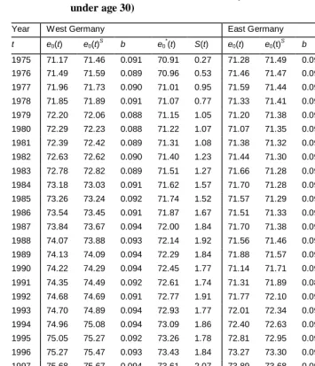
Table 2 presents the estimates of parameter µ0(t) and the average of parameter b
for the analyzed populations from 1975 to 2004, as done by Bongaarts and Feeney (2002) for the US, Sweden, Japan, and France. The estimates for b for the whole series of single observation years are shown in Tables 3 and 4, respectively. Corresponding to
the observed death rates, µ0(t) declines over time for all four populations. Similar to
what is known for several other countries, the estimated values of b are close to 0.09 among males and 0.10 among females for both western and eastern Germany. During the observation period, the annual estimates of b vary only little over time in each of these populations, as can be seen from the standard deviation of b in Table 2 or from the single values in Tables 3 and 4, respectively. As with the populations analyzed by Bon-gaarts and Feeney (2002), the Gompertz model fits the observed adult death rates very
well, with the average variance explained (R2) being around 99 percent. This shows that
the proportionality (or “constant shape”) assumption is approximately valid and the indirect method as introduced by Bongaarts and Feeney (2002) can be applied.
Table 2: Estimates of the parameters of the Gompertz mortality change model, males and females, western and eastern Germany, 1975-2004
Average 1975-2004
µ0(1975) µ0(2004) b St. dev. b R2
western Germany, males 6.639 ( ·10-5 ) 2.276 ( ·10-5 ) 0.092 0.0023 0.997
eastern Germany, males 4.116 ( ·10-5 ) 2.211 ( ·10-5 ) 0.094 0.0029 0.994
western Germany, females 1.729 ( ·10-5 ) 4.322 ( ·10-6 ) 0.105 0.0036 0.984
eastern Germany, females 1.080 ( ·10-5 ) 4.254 ( ·10-6 ) 0.108 0.0043 0.991
Based on these data, I used a three-step procedure similar to the procedure
pro-posed by Bongaarts and Feeney (2002). First, I calculated the annual estimates of e0(t)
from 1950 to 2004 with life tables that have mortality under age 30 set to 0. Next, I smoothed the estimates by fitting a sixth degree polynomial, using the computer pro-gram Microsoft Excel. The resulting values for the smoothed time series for life
expec-tancy e0(t)S are provided in Tables 3 and 4, respectively. Figure 2 shows the
correspond-ing functions together with the original estimates for e0(t) with no mortality under age
30. It can be seen that the trends in e30 + 30 (what corresponds to setting mortality
be-low age 30 to 0) are very similar to the trends in e0, shown in Figure 1. They differ only
especially infant mortality) had a higher impact on overall life expectancy than it has had in years more recent. Note that the significant decrease in life expectancy at birth
e0(t) for East German men in 1990 diminishes in the smoothed values e0(t)S.
To estimate tempo-adjusted life expectancy e0*(t), the original values for e0(t) are
substituted by values e0(t)S derived from the polynomial functions. To finally solve
Equation (2) for e0*(t), I used the so-called Euler’s method, with S(1950) = 2 as the
initial condition for the differential equation. From Equation (1) then follows that
e0*(1950) can be directly estimated from e0(1950) – S(1950). For instance, for West
German males it follows that e0*(1950) = 71.28 – 2.00 = 69.28. This value represents
the assumed tempo distortion for mortality changes until the year 1950, which was equally set for all populations observed, and thus the female and male populations of West and East Germany. The results for the analyzed years after 1975 are not entirely insensitive to this assumed initial condition for the year 1950 but its effect on the
esti-mates is relatively weak.11 An application of Euler’s method leads to an estimate for the
tempo-adjusted life expectancy e0*(1951) for the next year from the equation:
(
)
[
]
{
1 exp (1950) (1950) (1950)}
)1950 ( ) 1951
( *
0 0
* 0 *
0 e b e e
e = + − − ⋅ S −
or generally written from
(
)
[
]
{
1 exp () () ()}
.) ( ) 1
( 0* 0 0*
*
0 t e t bt e t e t
e + = + − − ⋅ S− (3)
Equation (3) was used to estimate a complete time series of values for tempo-adjusted life expectancy at birth (with no mortality under age 30) until 2004 for western and eastern German females and males. For a more detailed derivation of Equation (3), see Luy (2005a).
Table 3: Estimates of e0(t), e0(t)S, b, e0*(t), and S(t) for single calendar years,
males, western and eastern Germany, 1975-2004 (no mortality under age 30)
Year West Germany East Germany
t e0(t) e0(t)
S
b e0
*
(t) S(t) e0(t) e0(t)
S
b e0
*
(t) S(t)
1975 71.17 71.46 0.091 70.91 0.27 71.28 71.49 0.098 71.36 -0.08 1976 71.49 71.59 0.089 70.96 0.53 71.46 71.47 0.093 71.37 0.09 1977 71.96 71.73 0.090 71.01 0.95 71.59 71.44 0.094 71.38 0.21 1978 71.85 71.89 0.091 71.07 0.77 71.33 71.41 0.094 71.39 -0.06 1979 72.20 72.06 0.088 71.15 1.05 71.20 71.38 0.095 71.39 -0.19 1980 72.29 72.23 0.088 71.22 1.07 71.07 71.35 0.097 71.39 -0.31 1981 72.39 72.42 0.089 71.31 1.08 71.38 71.32 0.092 71.38 -0.01
1982 72.63 72.62 0.090 71.40 1.23 71.44 71.30 0.092 71.38 0.06 1983 72.78 72.82 0.089 71.51 1.27 71.66 71.28 0.093 71.37 0.29 1984 73.18 73.03 0.091 71.62 1.57 71.70 71.28 0.094 71.36 0.34 1985 73.26 73.24 0.092 71.74 1.52 71.57 71.29 0.096 71.35 0.21 1986 73.54 73.45 0.091 71.87 1.67 71.51 71.33 0.095 71.35 0.16 1987 73.84 73.67 0.094 72.00 1.84 71.70 71.38 0.094 71.35 0.35 1988 74.07 73.88 0.093 72.14 1.92 71.56 71.46 0.092 71.35 0.21 1989 74.13 74.09 0.094 72.29 1.84 71.88 71.57 0.093 71.36 0.52
1990 74.22 74.29 0.094 72.45 1.77 71.14 71.71 0.090 71.38 -0.24 1991 74.35 74.49 0.092 72.61 1.74 71.31 71.89 0.087 71.41 -0.10 1992 74.68 74.69 0.091 72.77 1.91 71.77 72.10 0.090 71.45 0.32 1993 74.70 74.89 0.094 72.93 1.77 72.01 72.34 0.092 71.51 0.51 1994 74.96 75.08 0.094 73.09 1.86 72.40 72.63 0.090 71.58 0.82 1995 75.05 75.27 0.092 73.26 1.78 72.81 72.95 0.094 71.67 1.14 1996 75.27 75.47 0.093 73.43 1.84 73.27 73.30 0.092 71.78 1.49 1997 75.68 75.67 0.094 73.61 2.07 73.89 73.68 0.095 71.91 1.98
Table 4: Estimates of e0(t), e0(t)S, b, e0*(t), and S(t) for single calendar years,
females, western and eastern Germany, 1975-2004 (no mortality under age 30)
Year West Germany East Germany
t e0(t) e0(t)
S
b e0
*
(t) S(t) e0(t) e0(t)
S
b e0
*
(t) S(t)
1975 76.84 77.10 0.101 75.59 1.25 75.91 76.07 0.106 75.34 0.57 1976 77.17 77.28 0.100 75.73 1.43 76.15 76.10 0.105 75.41 0.73 1977 77.74 77.48 0.102 75.88 1.86 76.53 76.14 0.103 75.48 1.05 1978 77.74 77.68 0.101 76.03 1.71 76.34 76.18 0.106 75.55 0.79 1979 78.03 77.89 0.099 76.18 1.85 76.40 76.23 0.106 75.61 0.79 1980 78.27 78.11 0.102 76.34 1.93 76.17 76.28 0.105 75.68 0.50 1981 78.34 78.33 0.102 76.50 1.84 76.37 76.35 0.105 75.74 0.63
1982 78.57 78.56 0.102 76.67 1.90 76.57 76.43 0.105 75.80 0.77 1983 78.76 78.79 0.102 76.85 1.91 76.82 76.52 0.106 75.87 0.95 1984 79.23 79.01 0.102 77.03 2.20 76.85 76.64 0.107 75.93 0.92 1985 79.30 79.24 0.104 77.21 2.09 76.77 76.77 0.107 76.01 0.76 1986 79.47 79.45 0.106 77.40 2.07 76.73 76.93 0.112 76.08 0.64 1987 79.82 79.67 0.108 77.60 2.22 77.14 77.11 0.111 76.17 0.97 1988 80.02 79.87 0.105 77.80 2.22 77.17 77.31 0.108 76.27 0.90 1989 80.07 80.07 0.104 77.99 2.08 77.49 77.54 0.105 76.38 1.11
1990 80.05 80.25 0.105 78.19 1.87 77.44 77.80 0.103 76.49 0.95 1991 80.26 80.43 0.106 78.38 1.87 77.69 78.09 0.101 76.62 1.07 1992 80.59 80.59 0.104 78.58 2.02 78.38 78.40 0.108 76.76 1.62 1993 80.50 80.74 0.106 78.77 1.74 78.86 78.74 0.106 76.92 1.94 1994 80.78 80.89 0.107 78.96 1.82 79.18 79.10 0.118 77.10 2.08 1995 80.89 81.02 0.107 79.14 1.75 79.53 79.47 0.108 77.31 2.23 1996 80.98 81.15 0.106 79.32 1.66 79.86 79.86 0.105 77.52 2.35 1997 81.32 81.29 0.108 79.50 1.82 80.43 80.26 0.115 77.73 2.69