Numerical Simulation of Random Irregular Waves for
Wave Generation in Laboratory Flumes
Mohammad Janvad Ketabdari i *and Ali Ranginkaman ii
Received 30April 200; received in revised 22July 2008; accepted 13March 2009
ABSTRACT
Understanding of wave hydrodynamics and its effects are important for engineers and scientists. Important insights may be gained from laboratory studies. Often the waves are simulated in laboratory flumes do not have the full characteristics of real sea waves. It is then necessary to present reliable methods of wave generation in wave flumes. In this paper, the results of numerically simulated water waves using different methods are presented. A model was developed to simulate water wave profile using DSA, NAS and WNDF methods. The results showed that although DSA method provides better agreement between output and target spectra, it is associated with non realistic simulation of sea waves. In the other hand WNDF method involves better stochastic wave characteristics if a qualitative white noise is used. It is also possible to put some controls on wave characteristics as input to WNDF model.
KEYWORDS:
Random Irregular Waves, DSA Method, NSA Method, WNDF Method, White Noise
i* Corresponding Author, Assistant Professor, Faculty of Marine Technology, Amirkabir University of Technology, Tehran, Iran (Email: [email protected])
ii MSc in Ship Hydrodynamics, Faculty of Marine Technology, Amirkabir University of Technology Tehran, Iran (Email: [email protected])
1. INTRODUCTION
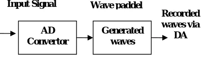
Wind waves are one of the prominent physical processes at upper boundary of the seas and oceans. These waves, which can travel beyond the direct effect of the generating forces, may interact with offshore structures far from the beach or coastal structures and sea bed at the near-shore zone. To design coastal and offshore structures, it is required to evaluate the effect of sea waves on the structures. To accomplish this mathematical and physical models are required. Therefore the problem has different features. On one hand the structure should be modeled properly. On the other hand the exciting force should be simulated. In some model tests monochromatic waves are used. However waves in fully developed seas are usually random and irregular and can be expressed by their energy spectrum over a range of frequencies. Hence ideal sine waves with a single frequency can not express all features of real sea waves. This may leads to misleading results. Therefore, it is necessary to generate irregular random waves for model studies of marine environment. Firoozkoohi and ketabdari (2007) designed an irregular wave maker for laboratory wave flume using random numerical waves as input [1]. Figure 1 presents the proposed system:
Figure 1: Proposed system of laboratory wave generation
2. IRREGULARWAVESYNTHESISMETHODS
The technology of wave generation in the laboratory has developed rapidly during the two past decades. It has benefited mainly from advances in control system theory and computer hardware. In past decades attempts have been made to generate laboratory waves which closely approximate natural wave trains. The techniques for synthesising irregular waves for laboratory studies can be categorised as follows:
2-1. SUPERPOSITION OF A FINITE NUMBER OF SINE WAVES
In this method the simulation is based on the superposition of many individual waves each of which has amplitudes consistent with the energy in the target spectrum and a random phase Φ as follows:
AD Convertor Input Signal
Generated waves
Recorded waves via
η
( )
t
c
ncos(
k x
nω
nt
n)
n N
=
−
+
=
∑
Φ
1
(1)
where:
c
n=
2 (
S f
n)
df
andω
n=
2
π
f
n so thatf
n=
f
n+
f
n−12
anddf
f
f
F
N
n n s
=
−
−1=
in which
F
s is sample frequency andN
is data number. The target spectrumS f
( )
may be specified by a theoretical curve or from actual ocean wave records. One of the disadvantages of this method is that it only reproduces the information stored in the spectrum (the wave amplitudes) and no phase information is included.2-2. DETERMINISTIC AND NON-DETERMINISTIC IRREGULAR WAVE TRAINS (DSA AND NSA METHODS
In order to employ the two simulation methods developed by Rice (1954) a surface wave target spectrum in the frequency domain is used [2]. In the Non-deterministic Spectral Amplitude (NSA) method, it is assumed that the fluctuations of a sea surface represent a stationary, ergodic process that has a Gaussian distribution and the energy distribution can be characterised with a spectrum. In this method the sea surface fluctuations at a point can be given as:
η
( )
(
cos
ω
sin
ω
)
/
t
a
a
n nt b
t
n N
n n
=
+
+
=
∑
0 1 2
2
(2)
where the first term is the mean and coefficients
a
n andb
n are independent random variables that have a normal distribution with zero mean and with a standard deviationn
σ
. In this method a sequence of paired numbersα
n andβ
n are generated randomly anda
n andb
n can be determined as follows:a
n=
α
nS f df
( )
n ,b
n=
β
nS f df
( )
n (3)Then a discrete time series is obtained using inverse
FFT on amplitudes
R
n=
a
n2+
b
n2and phases
θ
n=
a
nb
n−
tan (
1/
)
. Therefore, the only constraints placed on the simulation are the spectral density of the wave and this disregards the phase differences between the spectral components. In the Deterministic Spectral Amplitude (DSA) method it is also assumed that the sea surface has a Gaussian distribution and represented by the energy spectrum and the sea surface fluctuations can be given as:η
( )
cos(
ω
)
/
t
c
c
n nt
n N
n
=
+
−
=
∑
0 1 2
2
Φ
(4)
In this method a sequence of uniformly distributed random phases over the interval
0
≤
Φ
n≤
2
π
can be obtained by generating a sequence of random numbers uniformly distributed between 0 and 1 and multiplying them by2
π
. The values ofc
n can be obtained in terms of the discrete values of the target spectrum as:c
n=
2 (
S f
n)
df
. A discrete time series realisation can then be obtained using the inverse FFT on the above amplitudes and phases. Funke et al. (1988) referred to this method as the Random Phase (RPH) method [3]. This method is spectrally deterministic due to the amplitude spectrum being specified in terms of the Fourier amplitudes. In the NSA approach in order to assure a good statistical representation in the irregular wave time series, a lengthy time series must be produced. Therefore, rather than trying to find the worst condition, the lengthy test runs will increase the chance of occurrence of the relevant worst condition for each model test in the wave flume. However, in laboratory model simulations, lengthy runs are not only costly but also may cause some undesirable laboratory effects such as seiching in the flume [4].2-3. PROTOTYPE MEASUREMENT OF WIND WAVE TIME SERIES
In this method measured sea surface elevation time series can be scaled for laboratory reproduction. In this way some laboratories try to reproduce the prototype wave train as a useful tool for sea state synthesis. For example, Gravesen and Sorensen (1977) preferred this technique in their laboratory study [5]. This preference is based on the assumption that in the absence of full understanding of the natural sea state characteristics, reproduction of a sea state produces a margin of safety. However, the principle argument against this idea is that the limited samples of wave records taken at a special time and particular point in the sea may not be relevant to the worst condition of the underlying study structure.
2-4. FILTERING WHITE NOISE USING PROPER DIGITAL FILTERS (WNDF METHOD)
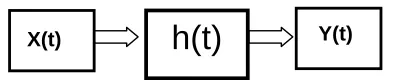
In method 5 a digital filter should be designed. Digital filter is a single input - single output (SISO) system [6].
This system is linear time invariant (LTI) and can be shown as in figure 2:
Y(t)=L(x(t))
Figure 2: A linear single input-output system
Considering X1(t) and X2(t) as two arbitrary inputs and a
,b two arbitrary real constants, this system is called linear if :
))
(
(
))
(
(
))
(
)
(
(
aX
1t
bX
2t
aL
X
1t
bL
x
2t
L
+
=
+
(5)The system is called time invariant if:
)
(
))
(
(
X
t
t
0Y
t
t
0L
−
=
−
(6)In which
t
0 is an arbitrary time shifting. A stochastic process is a rule that represents a functionf
(
t
,
ζ
)
fromt and
ζ
.For a stochastic process, first order distribution and first order density are defined as the following respectively [7]:}
)
(
{
)
,
(
x
t
p
x
t
x
F
=
≤
(7)x
t
x
F
t
x
f
∂
∂
=
(
,
)
)
,
(
(8)In which p{x} is the probability function. The average of a stochastic process for a stochastic variable x(t) is called Expected value as:
∫
−∞∞=
xf
x
t
dx
t
x
E
(
(
))
(
,
)
(9)Autocorrelation function is defined as:
)}
(
)
(
{
)
,
;
,
(
)
,
(
t
1t
2x
1x
2f
x
1x
2t
1t
2dx
1dx
2E
x
1t
x
2t
R
x=
∫ ∫
∞=
∞ − ∞ ∞ − (10)
Where
f
is stochastic variable and x(t
1)=x
1 and x(t2)=x
2. A stochastic processx
(
t
)
is called Strict-Sense Stationary (SSS), if it is statistically independent of distance from the origin [8]. In other words,x
(
t
)
isstatistically equal to
x
(
t
+
c
)
, where c is an arbitraryvalue. Also a stochastic process
x
(
t
)
is called Wide-Sense stationary (WSS) when the expected value (average) is constant:E
{(
x
(
t
)}
=
η
and its autocorrelation relates only with difference between1
t
andt
2(
τ
=
t
1−
t
2)
and independent oft
1andt
2 values:)
(
)}
(
*
)
(
{
x
t
τ
x
t
R
τ
E
+
=
(11)White noise is a noise with a power spectrum that is independent of frequency and its value at any frequency is:
2 )
(f q N0
Sw = = (12)
This noise is called white noise because the density spectrum of this process is widely distributed in the frequency domain as white light. Therefore autocorrelation function of white noise can be
represented as follows [9]:
) ( 2 ) ( )
(
τ
qδ
τ
N0δ
τ
Rw = = (13)
Figures 3a and 3b show spectrum and autocorrelation function of white noise:
Figure 3: a) White noise spectrum and b) Its autocorrelation function
It means that
R
xx(
z
)
can be obtained from the spectrumS
(
ω
)
. Considering the linear time invariantsystem with impulse response
h
(
t
)
as figure 4:Figure 4: A linear time invariant system with impulse response
)
(
t
h
If
x
(
t
)
is a WSS process, then the relation between output and input autocorrelation would be as below[10]:)
(
*
)
(
)
(
t
h
*t
R
t
R
xy=
−
xx (14))
(
*
)
(
)
(
t
h
t
R
t
R
yy=
xy (15)Leading to:
)
(
*
)
(
*
)
(
)
(
t
R
t
h
t
h
*t
R
yy=
xx (16)Taking Fourier transform from both sides of above equation we have:
2
)
(
)
(
)
(
*
)
(
)
(
)
(
f
S
f
H
f
H
f
S
f
H
f
S
yy=
xx=
xx (17)If the input of system is White noise with
q
=
1
then:1
)
(
,
)
(
)
(
)
(
=
q
=
S
f
=
R
xxτ
δ
τ
δ
τ
xx)
(
)
(
)
(
)
(
)
(
f
S
f
H
f
2H
f
S
f
S
yy=
xx⇒
=
yy (18)So, to achieve a process with a certain spectrum a system
2 0 N
)
(
f
S
0
f
(a) ) ( 20δτ
N
τ
)
(
τ
R
0
(b)with following transfer function can be defined:
0
)
(
,
)
(
)
(
f
=
S
f
H
f
=
H
≺
(19)If the input of such system is White noise, then the output of system will have the spectrum
S
(
f
)
.)
(
1
)
)
(
(
)
(
)
(
)
(
f
H
f
2S
f
S
f
2S
f
S
yy=
xx=
×
=
(20)3. SIMULATIONRESULTS
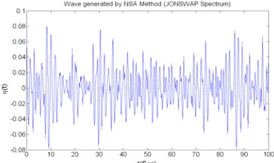
As mentioned in previous section if the transfer function of a filter is root of the spectrum and the input to this filter is white noise, then the output of the filter would be a random irregular wave that has the same spectrum. So a filter with a white noise input can be designed leading to an output which is desirable simulated wave (random irregular wave). Therefore based on the above mentioned algorithm a software was developed to generate random irregular waves by white noise filtering. Using JONSWAP as target spectrum sample irregular random waves were generated. Figures 5 to 7 show the time histories of generated wave using different methods. It can be seen that the results of simulation are different wave time histories using different methods. However the time histories alone can not give us further information about these waves. Figures 8 to 10 compare these wave energy spectra with target ones. This may be considered as a criterion for accuracy of the method. It is clear from these figures that in DSA method the output spectrum fairly matches with target one. However in NSA and WNDF method it fluctuates around the target spectrum. Figures 11 to 13 present autocorrelation of generated waves for three methods. This can be considered as a criterion for evaluating randomness of the signals. It is evident from this graphs that autocorrelation function has a main lobe at about τ = 0 and very small adjacent lobes elsewhere
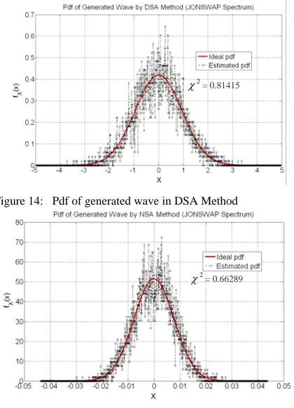
in all methods. Figures 14 to 16 compare the ideal and output probability density function for three cases. It can
be seen that the values of
χ
2 in different methods are 0.814, 0.663 and 0.577 respectively.Figure 5: Time histories of generated wave in DSA Method
Figure 6: Time histories of generated wave in NSA Method.
Figure 7: Time histories of generated wave in WNDF Method
Figure 8: Comparison of spectrum of generated wave and target spectrum In DSA Method
Figure 10: Comparison of spectrum of generated wave and target spectrum in WNDF Method
Figure 11: Autocorrelation of generated wave in DSA Method
Figure 12: Autocorrelation of generated wave in NSA Method
Figure 13: Autocorrelation of generated wave in WNDF
Method
Figure 14: Pdf of generated wave in DSA Method
Figure 15: Pdf of generated wave in NSA Method
Figure 16: Pdf of generated wave in WNDF Method
4. CONCLUSIONS
DSA, NSA and WNDF methods was employed to
simulate random irregular waves for numerical and laboratory models of marine environment. The well known spectral wave energy of JONSWAP was used as target. In WNDF method choosing the square root of the spectrum as transfer function of a filter and the input to this filter a white noise, a random irregular wave was generated. The time histories of generated waves using different methods show that apparently random irregular waves are obtained as output. However to asses the quality of generated waves the output spectra in three cases was compared with the target ones. The results showed that the DSA method, which is spectrally deterministic, offers easier matching of the peak spectral
2
χ = 0.81415
2
χ = 0.66289
2
frequency and the spectral shape [11]. It means that the DSA model simulates a uniform Gaussian white spectrum and therefore the constructed time series realisation will also closely match the target spectrum. Furthermore, DSA experimental runs can be much shorter due to the fact that the waves more likely to cause damage to the marine structures or to carry considerable sediment have been included in the wave time series. This can significantly reduce the cost of experimental work and, therefore, a wider variety of wave conditions can be tested. However as real sea states exhibit variations in spectral frequency between time series measurements, the DSA model results in irregular wave conditions that may be unrealistic in terms of natural sea states. The spectrum simulated by the NSA model fluctuates about the target spectrum within the bounds of probability. This method is spectrally non-deterministic because of the non-deterministicity of both amplitudes and phases. In WNDF method also output spectrum fluctuates around target one. This result is in fact desirable as realistic sea waves demonstrate a non-smooth spectrum. In addition the spectrum shows that the generated waves associated with wave energy in a range of frequencies which have the character of irregular sea
waves.
To be certain about the randomness of waves the autocorrelation function was used. The results showed that the generated waves are reasonably random. The comparison of power spectrum density function of output waves with ideal ones also shows the acceptable deviation. It should be noted that DSA and NSA methods simulation is in time domain. However WNDF method simulates the waves in frequency domain. The design of digital filters in the latter method is based on the spectral analysis and linear time invariant (LTI) systems, associated with strong mathematical and theoretical background. One of the most important advantages of this method is the possibility of placing additional constraints on specific characteristics such as number of waves in wave time series, frequency band, time domain, wave amplitude, wave energy, wave nonlinearity and other favorable wave characteristics. It is also possible to make the required filter using electronic hardwares. Therefore WNDF method can be used for wave simulation not only in the laboratory flumes but also in numerical and mathematical models of marine structures and coastal beaches.
5. REFERENCES
[1] R. Firoozkoohi, M. J. Ketabdari, (2008): "Design of irregular wave maker for marine laboratory", First Conference of Advances in Marine Industry, Amirkabir University of Technology, Tehran, Iran, 2007.
[2] S. O. Rice, (1944): “Mathematical analysis of random noise”, Bell System Tech. J., Vol. 23, 1944 and Vol. 24, 1945. (Reprinted in selected papers on noise and stochastic processes, N. Wax (Ed.), Dover Pub. Inc., New York, N. Y., 1954, pp. 123-144).
[3] E. R. Funke, and Mansard, and E. P. D. Dai, G., (1988): “Realisable wave parameters in a laboratory flume”, Proc. 21st
Int. Conf. Coastal Eng., ASCE, Vol. 1, pp. 835-848. [4] S. A. Hughes, (1993): Physical models and laboratory
techniques in coastal engineering, JBW printers & binders Pte. Ltd., London.
[5] H. Gravesen, and T., Sorensen, (1977): “Stability of rubble mound breakwaters”, Proc. 23rd PIANC Conf., Leningrad.
[6] D. Brook, and R. J. Wynne, (1988): Signal Processing Principles and Applications", Edward Arnold.
[7] J. S. Bendat, and A. G. Piersol, (1986): Random data analysis and measurement, John Wiley and Sons Inc., New York. [8] M. Kendall, and K. Ord, (1986): Time Series, Mc Graw_Hill
.Inc.
[9] S. Haykin, (1993): Communication Systems, John Wiley & sons Inc
[10] K. S. Shanmugan, and A. M. Breipohl, (1998): Random signals – Detection, Estimation, and Analysis John Wiley and Sons, inc.
[11] E.R. Funke, and E.P.D., Mansard, (1987):“A rationale for the use of the deterministic approach to laboratory wave generation”, Proc. 22nd