Print ISSN: 2383-451X Online ISSN: 2383-4501 Web Page: https://jpoll.ut.ac.ir, Email: [email protected]
Two-Dimensional Solute Transport with Exponential Initial
Concentration Distribution and Varying Flow Velocity
Thakur, C. K.1, Chaudhary, M.1, van der Zee, S. E. A. T. M.2, 3 and Singh, M. K.1*
1. Department of Applied Mathematics, Indian Institute of Technology (Indian School of Mines), Dhanbad-826004, Jharkhand, India
2. Ecohydrology, Soil Physics and Land Management, Wageningen University, P.O. Box 47, 6700 AA Wageningen, The Netherlands
3. School of Chemistry, Monash University, Melbourne, 3800 VIC, Australia
Received: 30.01.2019 Accepted: 22.05.2019
ABSTRACT: The transport mechanism of contaminated groundwater has been a problematic issue for many decades, mainly due to the bad impact of the contaminants on the quality of the groundwater system. In this paper, the exact solution of two-dimensional advection-dispersion equation (ADE) is derived for a semi-infinite porous media with spatially dependent initial and uniform/flux boundary conditions. The flow velocity is considered temporally dependent in homogeneous media however, both spatially and temporally dependent is considered in heterogeneous porous media. First-order degradation term is taken into account to obtain a solution using Laplace Transformation Technique (LTT) for both the medium. The solute concentration distribution and breakthrough are depicted graphically. The effect of different transport parameters is studied through proposed analytical investigation. Advection-dispersion theory of contaminant mass transport in porous media is employed. Numerical solution is also obtained using Crank Nicholson method and compared with analytical result. Furthermore, accuracy of the result is discussed with root mean square error (RMSE) for both the medium. This study has developed a transport and prediction 2-D model that allows the early remediation and removal of possible pollutant in both the porous structures. The result may also be used as a preliminary predictive tool for groundwater resource and management.
Keywords: ADE, Aquifer, Solute, Analytical solution, Numerical Solution.
INTRODUCTION
The transport and fate of solutes in the subsurface region has been major research area in the environmental, hydrological and soil-sciences. The contaminant sites pose a threat to the subsurface water system, surface water ecosystem, drinking water supplies, soils, and human health. Hence there is a need to provide fast contaminant remediation and quality monitoring of the
*
Corresponding Author, Email: [email protected]
groundwater system. Contaminant transport due to advection and dispersion in a porous medium is traditionally modeled by 1-D, 2-D and 3-2-D A2-DE with appropriate initial and boundary conditions. Advection-dispersion theory (ADT) is extensively explored through analytical solution, numerical simulation and experimental investigations of homogeneous and heterogeneous media during the mid-20th century.
modeling draw full attention to discuss various issues such as solute behaviour, concentration pattern etc., through numerical models, analytical models or both. Numerical and analytical solutions have its own limitation although these solutions are very much relevant for predicting contaminant concentration behaviour. Analytical solution provides closed form solution but it is usually limited with regard to the complexity only. These solutions are useful for benchmarking the numerical codes and solutions and even reduce computational effort as well. Accordingly, many one-dimensional analytical solutions were developed. Analytical solution of solute transport model equation (STME) was studied with temporally dependent dispersion coefficient (Logan, 1996; Maraqa, 2007; Kazezyılmaz-Alhan, 2008; Kumar et al., 2009; Singh et al., 2009; Hayek, 2016; Van Duijn & Van Der Zee, 2018). Also, the exact and approximate solutions of the one-dimensional advection-dispersion equation was explored in a heterogeneous porous media with a spatially dependent dispersion coefficient (Yates, 1992). The solution was obtained for a constant/flux boundary condition with asymptotic and exponential dispersion coefficients. Also, for a one-dimensional domain an analytical solution was provided for infinite domain and four different types of temporally dependent dispersion coefficients (Basha & El-Habel, 1993).
Two-dimensional situations were investigated for finite and infinite domains and diverse options for decay and sorption kinetics (Park & Zhan, 2001; Tadjeran & Meerschaert, 2007; Singh et al., 2010; Wang & Huang, 2011; Khebchareon, 2012; Cremer et al., 2016). An exact solution of the two-dimensional ADE was provided with a time dependent dispersion coefficient. Instantaneous and continuous point-source solutions were explored for constant, linear, asymptotic and exponentially varying dispersion coefficients (Aral & Liao, 1996).
A two-dimensional analytical solution of the ADE was presented with velocity dependent dispersion in an isotropic medium and with a constant/zero flux boundary condition (Broadbridge et al., 2002). Transient groundwater flow was discussed analytically and numerically with spatially dependent parameters in heterogeneous anisotropic porous medium (Belyaev et al., 2007).
In groundwater systems, a special case of two-dimensional transport is formed by aquifer-aquitard interactions and investigated the two-dimensional STME i.e., an aquifer-aquitard system by an averaged approximation method with first and third type boundary conditions (Zhan et al., 2009). They assumed longitudinal and transversal dispersions in the aquifer and vertical advection and diffusion in the aquitard (Tang et al.,1981). Applying a power series technique, an analytical solution of the two-dimensional ADE was derived with linear space-dependent dispersivities in both directions of a uniform flow field (Chen et al., 2008). For first- and third-type boundary conditions, an exact analytical solution were derived for the two-dimensional ADE in a cylindrical co-ordinates system and a finite domain (Chen et al., 2011). A new matrix technique was developed to solve the 2-D time dependent diffusion equation with Dirichlet type boundary conditions (Zogheib & Tohidi, 2016). Recently, using Green’s Function Method (GFM), an analytical solution of the two-dimensional ADT was proposed with space and time dependent longitudinal and transversal component of the velocity and dispersion coefficient for infinite horizontal groundwater flow (Sanskrityayn et al., 2018).
closed form analytical solution of the two-dimensional advection dispersion equation is derived by Laplace Transform Technique for a semi-infinite flow domain with spatially dependent initial and uniform/flux boundary conditions. In addition, analytical solution is compared with numerical solution obtained by Crank-Nicolson (CN) method. Accuracy of the results is discussed using root mean square error (RMSE).
Mathematical Modelling for Homogeneous and Heterogeneous Media
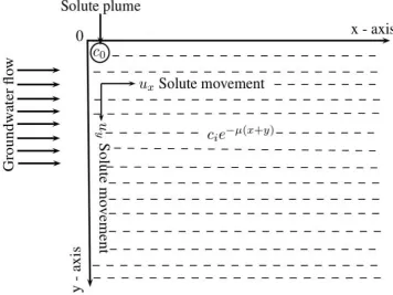
Two-dimensional ADE is considered to simulate solute contaminant transport in groundwater with a source in the horizontal plane at the origin of the domain (Figure 1). The semi-infinite length of impervious boundary is considered along the x- and y- directions. The origin of the Cartesian coordinate system is fixed for site of the contaminant plume. We have assumed that, the steady and unidirectional groundwater flow is horizontal i.e., along the x- direction. The solute concentration in the groundwater reservoir is assumed to be
constant at the beginning of contaminant transport. In the Cartesian co-ordinate system with uniform velocity, the transient two-dimensional advection dispersion equation with solid-liquid phase is formulated as
*
l d s l l
xx xy x l
l l d
yx yy y l l s
c c c c
D D u c
t t x x y
c c
D D u c c c
y x y
(1)
where, c1 [ML-3] is the liquid phase
concentration, cs [MM-1] is the sorbed mass
of solute contaminant in solid phase,
Dxx[L2T-1] and Dyy [L2T-1] are the dispersion coefficient components in principle direction, Dxy [L2T-1] and Dyx [L2T-1] are the cross dispersion coefficient components,
ux[LT-1] and uy[LT-1] are the seepage
velocity components in principle direction, [T-1] and *[T-1] are the first order decay rate for the liquid and solid phases respectively, d [ML-3] is the density of the
porous media and [-] is the porosity of geological media.
When contaminated groundwater flow is in reservoir, some solute components, such as polar organic solute compounds, heavy metals components, macromolecules particles and biogenic substance are sorbed by the solid phase. The sorption mechanism may include ionic exchange, physical adsorption and chemisorptions. A fundamental property of sorption system is the existence of equilibrium between solid and liquid phases, i.e., there exists the mathematical relationship as follows:
,
,
s l
c x t f c x t (2)
For linear equilibrium adsorption, transport equation can be re-written as follows;
*
l l l
xx xy x l
l l d
yx yy y l l s
c c c
R D D u c
t x x y
c c
D D u c c c
y x y
(3)
where, 1 d
f
R k
is retardation factor.
The groundwater flow field is uniform in a semi-infinite porous formation. Initially the domain contains solute with a spatially dependent function. A constant source is taken into consideration at the origin. Thus, initial and boundary conditions are written as follows:
, ,0
exp
l i
c x y c x y
0, 0, 0
x y t
(4a)
0, 0,
0l
c t c x0, y0,t0 (4b)
0
l x
c
x
and 0
l y
c
y
t0 (4c)
where, ci [ML-3] is the input source concentration and c0 [ML-3] is the uniform source concentration.
The effect of molecular diffusion is extended only due to the mechanical dispersion dominates the hydrodynamics dispersion process in solute transport mechanism. Instead, solute spreading in the
isotropic medium is characterized by a dispersion tensor Dij(Zheng & Bennett, 2002). Dispersion tensor can be estimated by
22 2
,
| |
i j
ij T ij L T
x y
u u
D U
U
U u u
and (i, j) (x, y)
(5)
where L and T are longitudinal and
transversal dispersivity parameter of porous media. ijis defined by 0,
1, ij
if i j if i j
.
In this study, we considered the flow of water to be uniform throughout the medium and in horizontal direction only and therefore in two-dimensional cases, cross dispersion component can be neglected. Hence Eq. (5) reduces to
,
xx L yy T
D U D Uand
0
xy yx
D D (6)
Case I. For a homogeneous porous
formation, we assumed two components of the velocity vector which are temporally dependent as follows:
0
x x
u u
mt and
0
y y
u u
mt (7)where ux0 [LT-1] and uy0 [LT-1] are initial seepage velocity components in the two principal directions i.e., x and y, respectively, m [T-1] is the flow resistance coefficient and (mt) is non-dimensional expression in the time variable.
It is common to assume that the mechanical dispersion coefficient (D) for homogeneous porous media varies nearly with the second power of seepage velocity (Bear, 1972). Hence, we obtained as
0
2
xx xx
D D
mt and
0
2
yy yy
D D
mt (8)where Dxx0[L2T-1] and Dyy0[L2T-1] are the
Using Eq. (7) and Eq. (8), Eq. (3) can be written as follows:
0
0 0 0
2 2 2 0 2 l l xx
l l l
yy x y l
c c
R
D mt
mt t x
c c c
D mt u u w c
y x y
(9) where, 0 mt , * * 0 mt
and *
0 0 0
d f
w k
By introducing a new time variable
1 1 0t
T
mt dt (10)Eq. (9) can be written as follows:
0
0 0 0
2 2 2 0 2 l l xx
l l l
yy x y l
c c
R D mt
T x
c c c
D mt u u w c
y x y
(11)
Introducing also a new space variable (Carnahan & Remer, 1984; Sanskrityayn & Kumar, 2018)
Z x y (12)
Eq (11) can be simplified as
20 2 0 0
l l l
l
c c c
R D mt u w c
T Z Z
(13)
where
0 0
0 xx yy
D D D and
0 0
0 x y
u u u
Introducing new spatial and temporal transformations as follows:
1Z dZ
mt
and (14)
1T dT
mt
Now transport Eq. (13) becomes
20 2 0 0
l l l
l
c c c
R D u w mt c
T Z Z
(15)
The initial and boundary conditions in terms of the above temporally and spatially dependent transformation can be written as
, ,0
exp
l i
c x y c
x y0, 0, 0
x y t
(16a)
0 0l
c ,T c Z 0, T 0 (16b)
l Z c 0 Z
T 0 (16c)
Now, we introduce a function G Z ,T
as
2 0 0 0 0 0 1 2 4 lc Z ,T G Z ,T
u u
exp Z w mt T
D R D
(17)
By using Eq. (17), the advective term is reduced in Eq. (15) and with the Laplace transforms technique for the assumed initial and boundary conditions; we get the solution as follows:
11
22
33
2 0 0 0 0 0 1 2 4 l
c Z ,T G Z ,T G Z ,T G Z ,T
u u
exp Z w T
D R D
(18) where
011 1 1 1
0 0
1 1 1 1
2 2
c R
G Z ,T exp T Z erfc Z T
R D D T R
0
1 1 1
0 0
1 1 1 1
2 2
c R
exp T Z erfc Z T
R D D T R
(19)
0 2 022 2 2 2
0
1
2 2
i
c D R D
G Z ,T exp T Z erfc Z T
R D T R
2
0 0
2 2 2
0
1
2 2
i
c D R D
exp T Z erfc Z T
R D T R
0 0 0 233 0 0
0 0
2 2
i
u D u
G Z ,T c exp Z T
D R D
(21)
2
0 0
1 0 2 0
0 0
4 2
u u
w ,
D D
(22)
This section described the numerical model of two-dimensional transport equation for homogeneous media. Numerical modeling of contaminant transport and groundwater flows was explored (Khebchareon, 2012; Chatterjee & Singh, 2018). In this work, Crank-Nicolson scheme is adopted for solving solute transport equation numerically and the following transformation is used:
1
Z 1 exp Z (23)
Thus, Eq. (15) - (16c) are transformed as
2 2 l l 0 2 1 l1 1 l
1
C C
R D 1 Z
T Z
C
u 1 Z w C
Z (24)
where, u1= D0 +u0
Initial and boundary conditions are as follows:
2
1 0 1 1 1 0 1 0 0 l a
C Z , C exp mt log ;
Z
Z , T
(25a)
0 1 0 0l b
C ,T C ; Z , T (25b)
1 1
0 1 0
l
C
; Z , T
Z
(25c)
Using Crank-Nicolson scheme, Eq. (24) is transformed as:
1 1 1 1 1
1 2 3
1 1
1 4 3
p ,q p,q p ,q
l l l
p ,q p,q p ,q
l l l
C C C
C C C
(26)
where,
2 2
0 1 0 1
1 2 1 1 2 2 1
1
1 1
2 2
0 1 0 1
3 2 1 1 4 2 1
1
1 1
1 1 1 2 1
2 4 2 2
1 1 1 2 1
2 4 2 2
D T u T D T w
Z Z , Z T
R Z R Z R Z R
D T u T D T w
Z Z , Z T
R Z R Z R Z R
(27)
and corresponding initial and boundary conditions are written as follows:
0 2 0 1 1 1 0 p , l a p
C C exp mt log ;
Z p (28a) 0 0 ,q l b
C C ; q (28b)
1 1
0
M ,q M ,q
l l
C C , q (28c)
where, pand qare corresponding to convenient distance and time steps, respectively. The domain
Z , T1
isdiscretize with interval length Z1 andT, respectively.
proportional to the square of the seepage velocity is used and therefore, we have
0 1 ax
x x
u u
mt and
0 1
y y
u u by
mt (29)where, a L 1 and b L 1represents the heterogeneity parameters.
and
0
2 2
1 ax
xx xx
D D mt and
0
2 2
1
yy yy
D D by mt (30)
Using Eq. (29) and (30), Eq. (3) can be written as follows:
0 0 0 0 2 2 2 2 2 2 1 2 0 1 1 1 1 l l xx l yy l x l y l c c RD ax mt
mt t x
c
D by mt
y c
u ax mt
x c
u by mt c
y (31)
where the coefficient of the advection term and decay rate are given as
0
0 1 2 1 xx x aD mt mt u ,
0
0 2 2 1 yy y bD mt mt u and 0 0 * 0 aux buy 0 0 kd
With the following spatial transformation
1 log 1
X ax
a
and
1 log 1 Y by b (32)Eq (31) can be rewritten as follows:
0 0 0 0 2 2 2 3 2 4 0 l l xx l l yy x l y l c c R D mtmt t X
c c
D mt u mt
Y X
c
u mt c
Y (33)
where the coefficients of the advection terms are
0
0 3 1 xx x aD mt mt u
and
0
0 4 1 yy y bD mt mt u
Using the new time variable given in Eq. (10), Eq. (33) becomes
0 0 0 0 2 2 2 3 2 4 0 l l xx l l yy x l y l c cR D mt
T X
c c
D mt u mt
Y X
c
u mt c
Y (34)
We define a new space variable (Carnahan & Remer, 1984; Sanskrityayn & Kumar, 2018)
Z X Y (35)
Using Eq. (35), Eq. (34) can be written as follows:
2 0 2 5 0 l l l l c cR D mt
T Z c mt c Z (36)
where
5
mt ux0
3
mt uy0
4
mt and0 0
0 xx yy
D D D
For convenience, we introduce new spatial and temporal variables as
5 * 0 Z mt Z dZ mt
and
2 5 * 0 T mt T dT mt
(37)and transport Eq. (36) can be written as follows:
2
0 0
* * 2 * 2
5
l l l
l
mt
c c c
R D c
T Z Z mt
(38)
The initial and boundary conditions are transformed as
0 0
* *
0 0
,0
l i x y
c Z c exp u aD bD Z
* *
0, 0
Z T
0
0* l
c ,T c Z* 0,T* 0 (39b)
* * 0 l Z c Z * 0
T (39c)
We considered
* * * * 2 * * 0 0 0 20 0 5
, ,
1
2 4
l
c Z T G Z T
mt
u u
exp Z T
D R D mt
(40)
In similar manner, we obtained the solution as follows:
* * * * * * * *
1 2 3
2
* *
0 0
0 2
0 0 5
, , , ,
1
2 4
l
c Z T G Z T G Z T G Z T
mt
u u
exp Z T
D R D mt
(41)
2 2 * * 0 00 2 0 2
0 5 0 0 5
* * 0 1
2
* 0 *
0
* 2
0 0 5
1 1 4 4 , 2 1 1 2 4 mt mt u u
exp w T w Z
R D mt D D mt
c G Z T
mt u
R
erfc Z w T
D T R D mt
2 2 * * 0 00 2 0 2
0 5 0 0 5
0
2
* 0 *
0
* 2
0 0 5
1 1 4 4 2 1 1 2 4 mt mt u u
exp w T w Z
R D mt D D mt
c
mt u
R
erfc Z w T
D T R D mt
0 0 0 0
0 0
2
* *
0
0 0 0 0
0 0
* * 2
* 0 *
0 0 * 0 0 1 1 2 2 , 2 1 1 2 2
x y x y
i
x y
D
exp u aD bD T u aD bD Z
R D D
c G Z T
D R
erfc Z u aD bD T
D T D R
(42)
0 0 0 0
0 0
2
* *
0
0 0 0 0
0 0
* 0 *
0 0 * 0 0 1 1 2 2 2 1 1 2 2
x y x y
i
x y
D
exp u aD bD T u aD bD Z
R D D
c
D R
erfc Z u aD bD T
D T D R
(43)
0 0
0 0
2
* * * 0 *
3 0 0 0 0
0 0
1 1
, exp
2 2
i x y x y
D
G Z T c u aD bD Z u aD bD T
D R D
(44)
By using similar procedure, discretized equation for heterogeneous medium is
obtained as follows:
1 1 1 1 1 1 1
1 2 3 1 4 3
p ,q p,q p ,q p ,q p,q p ,q
l l l l l l
C C C C C C
(45)
2 0 2
0 0 1
1 2 2 2 2 2 2
2
2 2
2 0 2
0 0 1
3 2 2 2 4 2 2
2
2 2
1
1 1 1 2 1
2 4 2 2
1
1 1 1 2 1
2 4 2 2
* * *
*
* * *
*
D
D T T D T w
Z Z , Z T
R Z R Z R Z R
D
D T T D T w
Z Z , Z T
R Z R Z R Z R
(46)
and
* 2
Z 1 exp Z
and initial and boundary conditions are as follows:
0 0
0
0 0
2
1 1 0
p ,
l a x y
p
C C exp u aD bD log ;
Z
p
(47a)
0
0 ,q
l b
C C ; q (47b)
1 1
0
M ,q M ,q
l l
C C , q (47c)
where, pand qare corresponding to distance and time, respectively. The domain (Z2, T*) are discretized with interval length Z2 and T*, respectively.
RESULTS AND DISCUSSION
Several analytical solutions for the 2-D solute transport equation with spatial and temporal dependent transport parameters have been reported in the literature. This section provides verification of the proposed analytical solution given by Eq. (16) for homogeneous and Eq. (34) for
heterogeneous porous media in the domain
0x km( ) 1 and 0 y km( ) 1 . We
computed the concentration distribution behaviour for an exponentially increasing or decreasing type velocity patterns. In the Himalayans basin region, the groundwater velocity in both principal directions decreases as a function of time after the snow melts. A representation that follows an exponential decrease reasonably characterizes this time dependency, as
0
x x
u u exp mt and
0
y y
u u exp mt
Solute dispersion is complicated in heterogeneous porous media at the macroscopic level because dispersion coefficient increases with seepage velocity of groundwater at different location. Symmetry analysis of this complication is illustrated in Table 1. Through this table, we show that temporal fluctuations in the magnitude of the seepage velocity that may enhance dispersion in principal direction for heterogeneous porous media.
Table1. Values of seepage velocity and its corresponding dispersion coefficient components with different location in the heterogeneous geological structure (Sandstone type aquifer) with dispersion theory
, 2 ,
D x t u x t along principal directions.
Case I. Variation of longitudinal seepage velocity and dispersion coefficient components are
0 1
x x
u u ax mt and
0
2 2
1 xx xx
D D ax mt respectively at different locations.
Parameters x=0 x=0.2 x=0.4 x=0.6 x=0.8 x=1.0
, x
u x t
0 0.20
x
u 0.24 0.28 0.32 0.37 0.41
, xx
D x t Dxx00.02 0.03 0.04 0.05 0.06 0.08
, xxD x t
0 0.04
xx
D 0.06 0.08 0.10 0.13 0.16
Case II. Variation of transverse seepage velocity and dispersion coefficient components are
0 1
y y
u u by mt and
0
2 2
1 yy yy
D D by mt respectively.
Parameters y=0 y=0.2 y=0.4 y=0.6 y=0.8 y=1.0
, y
u y t
0 0.10
y
u 0.15 0.21 0.26 0.31 0.37
, yyD y t Dyy0 0.01 0.02 0.04 0.06 0.10 0.13
, yy
Table 2. The Default Parameter values
Parameters Value
Solute concentration in inflow reservoir (C0) 1.0mg/km3
Input source concentration (Ci) 0.001mg/km
3 Initial seepage velocity component in principle direction (
0
x
u and
0
y
u ). 0.2 km/yr and 0.1 km/yr Initial dispersion coefficient component in principle direction (
0
xx
D and Dyy0). 0.02 km
2
/yr and 0.01 km2/yr
Resistive coefficient (m). 0.15 /yr
First order decay rate for solid phase (0). 0.2 /yr
First order decay rate for liquid phase (0*). 0.6 /yr
Porosity of sandstone aquifer 0.30
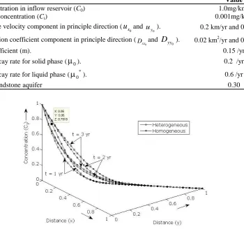
Fig. 2. Schematic diagram of concentration profile in the homogeneous and heterogeneous medium (sandstone type aquifer) for different time intervals (1t ( yr )3).
In hydrological sciences, the various geological properties of porous formation take part in solute contaminant transport through its pores. Figure 2 demonstrates the concentration distribution pattern for the homogeneous and heterogeneous medium for a sandstone (0.30) aquifer at time 1, 2 and 3yr, respectively. The same concentration values occur at the source point of domain in both homogeneous and heterogeneous porous medium. The concentration increases as a function of time and decreases with increasing distance. In case of a heterogeneous medium, initially the concentration values are smaller than that for the homogenous medium for all time. For both principal directions of flow, the concentration pattern becomes the same for both mediums.
Effect of variation in velocity pattern
Figure 3(a) illustrates the difference between sinusoidal and exponential (increasing and decreasing) type velocity patterns in a homogeneous aquifer (sandstone) for fixed time (t6yr).Intrinsic to the initial and boundary conditions, the concentration decreases smoothly from the maximum value at the origin to smaller values at larger distances. The curves for increasing and decreasing velocity appear to differ little, but show a much farther penetration of the concentration front than for the sinusoidal velocity.
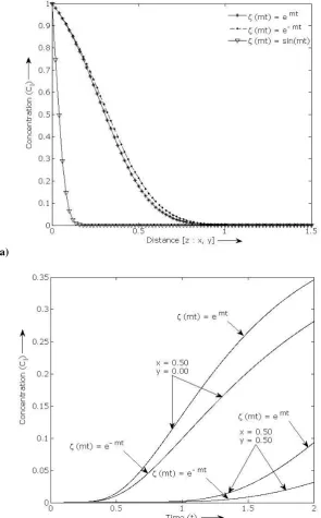
The curves presented in Figure 3(b) correspond to the pollutant concentration and time for different positions with exponential velocity patterns (
0 , 0
mt mt
x x y y
0 , 0
mt mt
x x y y
u u e u u e ). Results are shown for
two locations (x0.50, y0.00and
0.50, 0.50
x y ) for these exponential velocity component patterns. It is apparent that the initial breakthrough at these points is
earlier for the case of increasing velocity, and that it occurs later for the position with equal
x- and y- coordinates, as it is farther away from the origin than the location on the y-
axis.
(a)
(b)
Fig. 3. (a) Concentration distribution patterns in the homogeneous medium (Sandstone) with the different types of velocity patterns for fixed time (t=6yr). (b) Contaminant concentrations versus time for different spatial point with different velocity components patterns (
0 , 0
mt mt
x x y y
u u e u u e and
0 , 0
mt mt
x x y y
u u e u u e ) in the homogeneous porous media (Sandstone). These figures were drawn for
*
2.49, 0.30, 0.06, 0.02
Effect of variation with spatial point
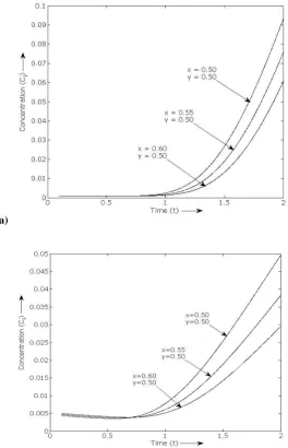
Figure 4(a) plots concentration as a function of time for an exponential decreasing source with different x- positions (x=0.50, 0.55, 0.60) and for a fixed y- position (y=0.50). The concentration increases faster as a point is closer to the origin. At location x= 0.60,
y= 0.50 have leads to a slower solute transport process. The output concentration illustrates in Table 4for both the porous medium. In Figure 4(b) concentration breakthrough at different positions is shown for a heterogeneous aquifer subject to
heterogeneity a=1, b= 2.6. Since heterogeneous aquifer are characterized by a complex heterogeneous spatial structure that strongly affect the dynamics of solute transport and fluid flow. For the heterogeneous aquifer, it is apparent that the concentration initially is larger than for the homogeneous one, and that it slowly decreases till a time of about 0.7 yr. After that, it increases for all shown points, and faster as the points are closer to the origin. The concentration values are provided in Table 4.
(a)
(b)
Fig. 4. (a) Concentration scales for an exponential source input in the homogeneous porous medium with different positions. (b) Concentrations distribution in the heterogeneous porous medium (Sandstone
aquifer with heterogeneity a=1, b= 206) for different positions. The parameters used are
0 0.20, 0 0.10, 0 0.02, 0 0.01
x y xx yy
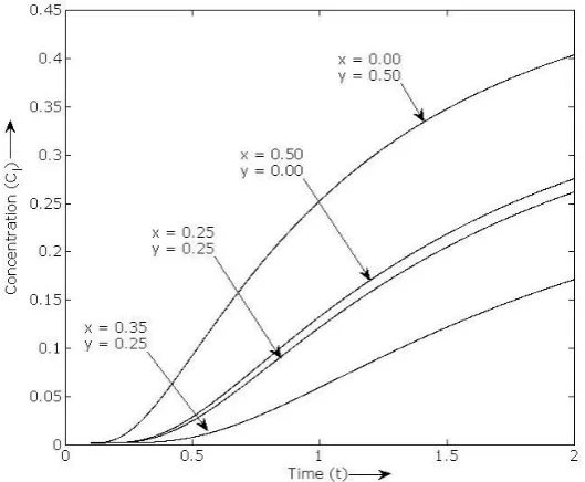
Figure 5 addresses the breakthrough curves (BTC) of concentration pattern subject to a temporally exponential decreasing velocity Eq. (29) for heterogeneous geological porous media. From this figure, the model results show that in aquifer filtration, the contaminant migration increase further in the presence of the organic matter and many bacterial particles. The contaminant zone after t=1yr
of heterogeneous layer is originated from the water flow with a high contaminant concentration level. The concentration level decreases with the increasing value of
x- positions (x=0.25, 0.35) in the case of constant y- position (y= 0.25). Also, the concentration pattern corresponding to the location (x= 0.00, y= 0.50) shows much more variation with increment in time than at the location (x= 0.50, y= 0.00).
Figure 6(a) and 6(b) illustrate the 2D surface plots of the concentration distribution for a homogeneous and a heterogeneous porous medium, respectively at fixed time (t= 4yr) for the sandstone aquifer.
The concentration values initially increase from the source point of the
domain and beyond this, concentration values decrease along principal directions of flow observed for color bar in Figure 6(a). As Figure 6(b) predict, the concentration surface in the heterogeneous porous medium decrease faster than for homogeneous one of Figure 6(a).
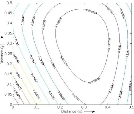
Figure 7 predicted the contour representation of relative solute concentration distribution in heterogeneous medium for sandstone (aquifer) formation. The concentration value attains the same along with the slope of the concentration and the value of concentration increases successively from the origin of the domain at fixed time (t= 4yr).
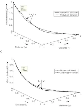
The concentration distribution patterns of both the porous structure are explained with the help of table and figures. The results obtained using analytical methods were compared with numerical one for both the porous media as shown in Figure 8 (a) and (b). It is observed that difference between the concentration values at different locations in homogeneous and heterogeneous porous media is almost negligible.
Fig. 5. Relative solute concentration profile of contaminant in the heterogeneous porous media (Sandstone aquifer = 2.49, = 0.30) for the different position. Parameter estimates are c0= 1.0, ci= 0.001, a= 1 and b=
(a)
(b)
Fig. 6. (a) The predicted concentration distribution surface curve in homogeneous soil columns for sandstone type aquifer at fixed time (t= 4yr). (b) The surface curve of solute concentration distribution in
heterogeneous layer for sandstone type aquifer at fixed time (t= 4yr).
a)
(b)
Fig. 8. (a) Comparison of the proposed analytical solution with the numerical solution at (t= 6yr) for the homogenous porous media using the best-estimated parameters. (b) Comparison of concentration distribution pattern through the analytical approach with the numerical solution at a fixed time (t= 6yr) for the heterogeneous porous media.
The accuracy and efficiency of the numerical solution is discussed with root mean square error (RMSE) defined as:
2 1
1 N i i
RMSE c
N
where, c canalyticalcnumericaland given below in Table5.
Table 5. RMSE for the homogeneous and heterogeneous mediums at t= 6yr duration.
Medium
Location
Homogeneous Heterogeneous
Analytical Values (Canalitical)
Numerical Values (Cnumerical)
Analytical Values (Canalitical)
Numerical Values (Cnumerical)
x=0.1=y 0.6812 0.6408 0.5391 0.5692
x=0.2=y 0.4516 0.4031 0.3110 0.3118
x=0.3=y 0.2645 0.2480 0.1814 0.1546
x=0.4=y 0.1156 0.1484 0.1014 0.0553
x=0.5=y 0.0329 0.0857 0.0524 0.0087
x=0.6=y 0.0068 0.0471 0.0249 0.0004
x=0.7=y 0.0025 0.0240 0.0115 0.0002
x=0.8=y 0.0020 0.0108 0.0063 0.0002
x=0.9=y 0.0019 0.0033 0.0055 0.0002
CONCLUSION
In this present paper, two-dimensional transport of solute is discussed in homogeneous and heterogeneous geological deposits. Analytical solution is developed by using the Laplace transformation technique for the case of spatially dependent initial and flux boundary conditions. For such situations, the concentration decreases rapidly in the direction of flow, but builds up with increasing time. By varying the initial and boundary conditions and velocity field, a set of concentration profile can be generated. The analytical solutions enable the consideration of new benchmark cases for assessing the quality of numerical solutions. Error analysis is also made for homogenous and heterogeneous medium and root mean square error (RMSE) is found i.e., 0.0342 and 0.0728 respectively.
ACKNOWLEDGEMENT
Authors are thankful to Indian Institute of Technology (Indian School of Mines), Dhanbad for providing financial support to doctoral students under the JRF scheme. Also, we are thankful to the editor and learned referee for their valuable suggestions which helped to improve the quality of paper.
REFERENCES
Aral, M. M. and Liao, B. (1996). Analytical solutions for two-dimensional transport equation with time-dependent dispersion coefficients. J. Hydrol. Eng., 1(1); 20-32.
Basha, H. A. and El-Habel, F. S. (1993). Analytical solution of the one-dimensional time-dependent transport equation. Water Resour. Res., 29(9); 3209-3214.
Bear, J. (1972). Dynamics of fluids in porous media. (New York: Elsevier).
Belyaev, A. Y., Dzhamalov, R. G., Medovar, Y. A. and Yushmanov, I. O. (2007). Assessment of groundwater inflow in urban territories. Water Resour., 34(5); 496-500.
Broadbridge, P., Moitsheki, R. J. and Edwards, M. P. (2002). Analytical solutions for two-dimensional solute transport with velocity-dependent dispersion. Environmental mechanics: water, mass
and energy transfer in the biosphere, The Philip Vol., 145-153.
Carnahan, C. L. and Remer, J. S. (1984). Nonequilibrium and equilibrium sorption with a linear sorption isotherm during mass transport through an infinite porous medium: some analytical solutions. J. Hydrol., 73(3-4); 227-258.
Chatterjee, A. and Singh, M. K. (2018). Two-dimensional advection-dispersion equation with depth-dependent variable source concentration. Pollut., 4(1); 1-8.
Chen, J. S., Ni, C. F. and Liang, C. P. (2008). Analytical power series solutions to the two‐ dimensional advection-dispersion equation with distance-dependent dispersivities. Hydrol. Processes., 22(24); 4670-4678.
Chen, J. S., Chen, J. T., Liu, C. W., Liang, C. P. and Lin, C. W. (2011). Analytical solutions to two-dimensional advection-dispersion equation in cylindrical coordinates in finite domain subject to first-and third-type inlet boundary conditions. J. Hydrol., 405; 522-531.
Cremer, C. J., Neuweiler, I., Bechtold, M. and Vanderborght, J. (2016). Solute transport in heterogeneous soil with time-dependent boundary conditions. Vadose Zone J., 15(6); 2-17.
Hayek, M. (2016). Analytical model for contaminant migration with time-dependent transport parameters. J. Hydrol. Eng., 21(5); 04016009.
Kazezyılmaz-Alhan, C. M. (2008). Analytical solutions for contaminant transport in streams. J. Hydrol., 348(3-4); 524-534.
Khebchareon, M. (2012). Crank-Nicolson finite element for 2-D groundwater flow, advection-dispersion and interphase mass transfer: 1. Model development. Int. J. Numer. Anal. Model., Series B, 3(2); 109-125.
Kumar, A., Jaiswal, D. K. and Kumar, N. (2009). Analytical solutions of one-dimensional advection-diffusion equation with variable coefficients in a finite domain. J. Earth Syst. Sci., 118(5); 539-549.
Logan, J. D. (1996). Solute transport in porous media with scale-dependent dispersion and periodic boundary conditions. J. Hydrol., 184(3-4); 261-276.
Maraqa, M. A. (2007). Retardation of nonlinearly sorbed solutes in porous media. J. Environ. Eng., 133(12); 1080-1087.
Pollution is licensed under a "Creative Commons Attribution 4.0 International (CC-BY 4.0)" Sanskrityayn, A. and Kumar, N. (2018). Analytical
solutions of ADE with temporal coefficients for continuous source in infinite and semi-infinite media. J. Hydrol. Eng., 23(3); 06017008. Sanskrityayn, A., Singh, V. P., Bharati, V. K. and Kumar, N. (2018). Analytical solution of two-dimensional advection-dispersion equation with spatio-temporal coefficients for point sources in an infinite medium using Green’s function method. Environ. Fluid Mech., 18(3); 739-757.
Singh, M. K., Begam, S. Thakur, C. K. and Singh, V. P. (2018). Solute transport in a semi-infinite homogeneous aquifer with a fixed-point source concentration. Environ. Fluid Mech., 18(5); 1121-1142.
Singh, M. K., Singh, P. and Singh, V. P. (2010). Analytical solution for two-dimensional solute transport in finite aquifer with time-dependent source concentration. J. Eng. Mech., 136(10); 1309-1315.
Singh, M. K., Singh, V. P., Singh, P. and Shukla, D. (2009). Analytical solution for conservative solute transport in one-dimensional homogeneous porous formations with time-dependent velocity. J. Eng. Mech., 135(9); 1015-1021.
Tadjeran, C. and Meerschaert, M. M. (2007). A second-order accurate numerical method for the two-dimensional fractional diffusion equation. J. Comput. Phys., 220(2); 813-823.
Tang, D. H., Frind, E. O. and Sudicky, E. A. (1981). Contaminant transport in fractured porous media: Analytical solution for a single fracture. Water Resour. Res., 17(3); 555-564.
Van Duijn, C. J. and van der Zee, S. E. A. T. M. (2018). Large time behaviour of oscillatory nonlinear solute transport in porous media. Chem. Eng. Sci., 183; 86-94.
Yates, S. R. (1992). An analytical solution for one-dimensional transport in porous media with an exponential dispersion function. Water Resour. Res., 28(8); 2149-2154.
Wang, K. and Huang, G. (2011). Effect of permeability variations on solute transport in highly heterogeneous porous media. Adv. Water Resour., 34(6); 671-683.
Zhan, H., Wen, Z., Huang, G. and Sun, D. (2009). Analytical solution of two-dimensional solute transport in an aquifer-aquitard system. J. Contam. Hydrol., 107; 162-174.
Zheng, C. and Bennett, G. D. (2002). Applied Contaminant Transport Modeling. Second ed. (Wiley: New York).