A numerical technique for solving a class of 2D variational problems
using Legendre spectral method
Kamal Mamehrashi
Department of Mathematics, Payame Noor University, P. O. BOX 19395-3697, Tehran, Iran.
E-mail: k [email protected] Fahimeh Soltanian∗
Department of Mathematics, Payame Noor University, P. O. BOX 19395-3697, Tehran, Iran.
E-mail: f [email protected]
Abstract An effective numerical method based on Legendre polynomials is proposed for the solution of a class of variational problems with suitable boundary conditions. The Ritz spectral method is used for finding the approximate solution of the problem. By utilizing the Ritz method, the given nonlinear variational problem reduces to the problem of solving a system of algebraic equations. The advantage of the Ritz method is that it provides greater flexibility in which the boundary conditions are imposed at the end points of the interval. Furthermore, compared with the exact and eigenfunction solutions of the presented problems, the satisfactory results are obtained with low terms of basis elements. The convergence of the method is ex-tensively discussed and finally two illustrative examples are included to demonstrate the validity and applicability of the proposed technique.
Keywords. Ritz method, Legendre polynomials, 2D Variational problems, Eigenfunction method.
2010 Mathematics Subject Classification. 65-XX, 65Kxx, 65K15.
1. Introduction
The calculus of variations investigates methods that permit finding maximal and minimal values of a large number of problems arising in analysis, mechanics and ge-ometry. The problems which consist the investigation of extremum for a function are called variational problems [7, 23]. It began to develop in 1696 and became an independent mathematical discipline with its own methods of investigation after the fundamental works of Euler (1707-1783), whom we may justifiably consider the founder of the calculus of variations [7]. Methods of solving variational problems, i.e. problems involving the investigation of functionals for maxima and minima, are extremely similar to the methods of investigating functions for maxima and minima [7,8].
The three problems, brachistochrone, geodesics and isoperimetric have played im-portant roles in the development of calculus of variations [6, 7]. In recent years,
Received: 18 February 2018 ; Accepted: 10 July 2018. ∗Corresponding author.
a growing interest has been appeared toward the application of different methods in various types of variational problems, and many new direct and numerical tech-niques have been introduced in the literature. For more details, we refer readers to [1,3,4, 5,9,10,11,12,17,18,19,22].
In this paper, we introduce an efficient numerical method to solve variational problems for functionals dependent on two independent variables in the following form
min J[z(x, y)] =
∫ b
0
∫ a
0
F(x, y, z,∂z ∂x,
∂z
∂y)dxdy, (1.1)
with the given boundary conditions
z(0, y) =f1(y), z(a, y) =f2(y), z(x,0) =g1(x), z(x, b) =g2(x), (1.2)
where the functionF is a three times differentiable function of its arguments. Let us assume that a function z = z(x, y) is being sought that is continuous together with its derivatives up to order two inclusive in the domainD. Furthermore, assume that the values on the boundary Σ of D are given and yield a minimum of the functional (1.1). The Ritz method is one of the most widely used direct variational methods which we use for approximation of the function z(x, y) to minimize the functional (1.1) [7, 8]. According to the Ritz method, we approximate the function
z(x, y) with the Legendre polynomial basis and the unknown coefficients such that the function z(x, y) satisfies initial and boundary conditions. Then by substituting the approximate function in the given cost functional, we obtain a nonlinear algebraic equation in terms of the unknown coefficients which should be optimized. By taking the necessary conditions for optimality into account, an algebraic system of equations will appear. The obtained system is solved for finding the unknown coefficients. The main advantage of the Ritz method is that the boundary conditions (1.2) are imposed at the end points of the interval. Moreover, only a small number of bases are needed to obtain a satisfactory result.
The organization of the rest of this paper is as follows. In section 2, we introduce some preliminaries required for our subsequent development. The numerical solution of the problem by Ritz method is presented in section 3. The convergence of the presented method is considered in section 4. To present a clear overview of the method, we select two examples in section 5. We compare the numerical results with analytical solution for Example5.1and eigenfunction method for Example5.2. A conclusion is presented in section 6.
2. Preliminaries
In this section, we briefly present some properties of Legendre orthonormal poly-nomials, function approximation and then state the Ritz method.
2.1. Legendre Polynomials. LetLj(r) denotes the Legendre polynomial of order
jon the interval [−1,1]. These polynomials can be derived by the following recessive relation known as Bonnet’s recursion formula
Lj+1(r) = 2j+ 1
j+ 1 rLj(r)−
j
whereL0(r) = 1, L1(r) =r. By change of variablex= 2
ar−1, we can easily obtain
the well-known shifted Legendre polynomials on interval [0, a],
La,j+1(x) =
2j+ 1
(j+ 1)a(2x−a)La,j(x)− j
j+ 1La,j−1(x), j= 1,2,3, ..
La,0(x) = 1, La,1(x) = 2x
a −1.
Now definepj(x) =
√
2j+ 1
a Lx,j, j = 1,2, ... We obtain the orthonormal Legendre
polynomials on the interval [0, a], that is,
∫ a
0
pi(x)pj(x)dx=δi,j,
whereδi,j is the Kronecker delta.
The analytical form of the shifted Legendre polynomials pj(x) of degree j in the
interval [0, a] is defined by [2]
pj(x) = 1 2j
[j2]
∑
l=0 (−1)l
( j l
)(
2j−2l j
)
sj−2l, s= 2
ax−1. (2.1)
2.2. Function Approximation. First, let us introduce a theorem. This theorem exploits the best approximation of a function in an inner product space.
Theorem 2.1. LetGbe an inner product space and L̸= Øbe a convex subset which
is complete (in the metric induced by the inner product). Then for every giveng∈G
there exists a uniqueh∗ ∈Lsuch that
minh∈L∥g−h∥=∥g−h∗∥.
Proof. [13].
Now let ∆ = [0, a]×[0, b]. Suppose that{pi(x)pj(y)}n,mi,j=0is a subset ofL2(∆) out of double product Legendre polynomials. Define
Λn,m= Span{pi(x)pj(y)|0≤i≤m, 0≤j ≤n}, m, n∈N ∪
{0}.
Letf be an arbitrary function inL2(∆). Since Λn,mis closed in the complete space L2(∆) so it is complete. Therefore, according to Theorem (2.1), there is a unique best approximation out of Λn,m likeσn,mwhich satisfies in the theorem’s condition,
that is
∀s(x, y)∈Λn,m, ∥f−σn,m∥2≤ ∥f−s∥2,
where∥f∥2=
√
< f, f >.
Sinceσn,m∈Λn,mso we can find the real coefficientsaij, i= 0,1, ..., n, j= 0,1, ..., m
such that
σn,m(x, y)≃ n ∑
i=0
m ∑
j=0
where the shifted Legendre coefficient matrixA, vectorsPn andPm are given by A=
a00 a01 · · · a0m a10 a11 · · · a1m
..
. ... · · · ...
an0 an1 · · · anm
, Pn=
p0(x) .. . .. .
pn(x)
, Pm=
p0(y) .. . .. .
pm(y)
and the real coefficients can be specified uniquely as follows [13]:
aij =< pi(x)pj(y),σn,m(x, y)>=
∫ a
0
∫ b
0
σn,m(x, y)pi(x)pj(y)dxdy,
i= 0, ..., n, j= 0, ..., m.
2.3. The Ritz Method. The underlying idea of the Ritz method is that the values of a functional
J[y(x)] =
∫ b
a
f(x, y, y′)dx, (2.3)
on the space of all continuously differentiable functions satisfying
y(a) =c0, y(b) =c1, (2.4)
are considered not on arbitrary admissible curves of a given variational problem but only on all possible linear combinations as a finite series with constant coefficients. In Ritz’s method, we seek a solution to the problem of minimization of the functional (2.3), with boundary conditions (2.4), in the form
yn(x)≃ n ∑
i=1
ciχi(x) +χ0(x), (2.5)
such that χ0(x) satisfies (2.4), that is, χ0(a) = c0, χ0(b) = c1. All the remaining functions satisfy the corresponding homogeneous conditions, i.e. in the case at hand,
χi(a) =χi(b) = 0, i= 1, ..., n. Theci are constants. The function y∗n(x) that mini-mizes (2.3) on the set of all functions of the form (2.5) is called thenth approximation of the solution by Ritz’s method [14].
Now letχi(x) =w(x)pi(x) then the formula (2.5) can be expressed as
yn(x)≃ n ∑
i=1
ciw(x)pi(x) +χ0(x), (2.6)
where w(x) satisfies the homogeneous conditions of the problem and pi(x) is the Legendre polynomial function.
Consider the following 2-dimensional functional
J[y(x, t)] =
∫ b
a ∫ d
c
f(x, t, y, yx, yt)dxdt, (2.7)
series
ynm(x, t)≃
n ∑ i=1 m ∑ j=1
cijw(x, t)pi(x)pj(t) +q(x, t), (2.8)
wherepi(x) andpj(t) are Legendre polynomials. Note thatw(x, t) is such that satisfies the homogeneous form of the specified essential boundary conditions. Furthermore
q(x, t) satisfies the initial and boundary conditions. It is easy to consider that the approximate solutionymn(x, t) satisfies the initial and boundary conditions [15,25].
3. Solving Two-Dimensional Variational Problem
Consider the cost functional
min
z J[z(x, y)] = ∫ b
0
∫ a
0
F(x, y, z,∂z ∂x,
∂z ∂y)dxdy,
with the given boundary conditions
z(0, y) =f1(y), z(a, y) =f2(y), z(x,0) =g1(x), z(x, b) =g2(x).
According to (2.8), the approximation of function ˆz(x, y) by considering the boundary conditions (1.2) is as follows
ˆ
z(x, y)≃
n ∑ i=0 m ∑ j=0
cijxy(x−a)(y−b)pi(x)pj(y) +q(x, y), (3.1)
such that
q(0, y) =f1(y), q(a, y) =f2(y), q(x,0) =g1(x), q(x, b) =g2(x).
The first derivatives of the function ˆz(x, y) with respect to x, yare expressed as
∂ˆz(x, y)
∂x ≃ n ∑ i=0 m ∑ j=0
cijy(y−b)pj(y)[(2x−a)pi(x) +x(x−a)p′i(x)] +∂q(x, y)
∂x ,
∂ˆz(x, y)
∂y ≃ n ∑ i=0 m ∑ j=0
cijx(x−a)pi(x)[(2y−b)pi(y) +y(y−b)p′i(y)] +∂q(x, y)
∂y ,
(3.2)
respectively. Substituting (3.2) and (3.1) in (1.1), the cost functionalJ[ˆz(x, y)] can be approximated and it becomes a function asJ∗=J[C] innmreal unknown variables where C=
c00 c01 · · · c0m c10 c11 · · · c1m
..
. ... · · · ...
cn0 cn1 · · · cnm .
Now the necessary conditions for the minimum of the approximated functionalJ∗are
∂J∗ ∂cij
= ∂J[C]
∂cij
The aforementioned algebraic system can be solved forcij, i = 1, .., n, j = 1, .., m
directly. By determining the matrixC, we can obtain the approximate value of ˆz(x, y) from (3.1).
4. Theoretical Analysis
In this section, we will provide theoretical analysis of the proposed method for problem (1.1)-(1.2). We will show that with increase in the number of Legendre polynomials basis m, n in (3.1), the approximate value of the J approaches to its exact value. This fact is shown in Theorem4.3. Here we construct our function space and present some needed lemmas.
Consider the Banach space (E(∆),||.∥) as follows
E(∆) ={h(x, y)|his continuously differentiable on ∆},
||h(x, y)||=||h(x, y)||∞+||∂h(x, y)
∂x ||∞+||
∂h(x, y)
∂y ||∞.
Let Emn be the mn-dimensional linear subspace of the Banach space (E(∆),||.||)
spanned by the first mn of the functions {p0(x)p0(y), ..., pm−1(x)pn−1(y)}, that is, the set of all linear combinations of the form
{ m∑−1
i=0
n−1
∑
j=0
αijpi(x)pj(y)},
where the coefficientsα00, ..., α(m−1)(n−1) are arbitrary real numbers. Then, the re-striction of the functionalJ[z(x, y)] toEmnis a function ofmnvariablesα00, ..., α(m−1)(n−1) as
J[
m∑−1
i=0
n∑−1
j=0
αijpi(x)pj(y)]. (4.1)
We chooseα00, ..., α(m−1)(n−1)in such a way as to minimize (4.1), denoting the min-imum value ofJ byρmn and the element ofEmn which yields the minimum byzmn.
Lemma 4.1. The defined functionalJ :E(∆)→Rin (1.1), is uniformly continuous
on the Banach space(E(∆),||.||).
Proof. ϵ >0 is given. Let z∈E(∆) andδ >0. Now suppose thatz1 ∈E(∆) such
that
||z−z1||=||z−z1||∞+||
∂(z−z1)
∂x ||∞+||
∂(z−z1)
∂y ||∞< δ.
Considering our assumptions for the problem (1.1)-(1.2), the functionz(x, y) is
con-tinuous with its derivatives, hence the functionF(x, y, z,∂z ∂x,
∂z
∂y) is continuous [20]
then there existsδ(ϵ)>0 such that
||F(x, y, z,∂z ∂x,
∂z
∂y)−F(x, y, z1, ∂z1
∂x, ∂z1
provided that||z−z1||< δ=δ(ϵ). Therefore we have
|J[z(x, y)]−J[z1(x, y)]|< ϵ.
The next Lemma is a result from the Stone-Weierstrass Theorem [21].
Lemma 4.2. Suppose thatz(x, y)∈E(∆,||.||). There exists a sequence of polynomial
functions{pi(x)pj(y)}∞i,j=0∈E(∆)in which converges toz(x, y).
The convergence of the proposed method is provided by the following Theorem.
Theorem 4.3. Let ρ be the minimum of the functional J[z] on the Banach space
E(∆,||.||). Then we have
lim
(m,n)→(∞,∞)ρmn=ρ.
Proof. ϵ >0 is given. By the definition of ρfor anyϵ there exists az∗ ∈E(∆,||.||)
such that
J[z∗]< ρ+ϵ.
Now sinceJ[z] is continuous onE(∆,||.||) then we have
|J[z]−J[z∗]|< ϵ, (4.2)
provided that ||z −z∗|| < δ = δ(ϵ). According to Lemma 4.2, there is a linear combinationρmn of the formα00p0(x)p0(y) +...+α(m−1)(n−1)pm−1(x)pn−1(y) such that||ρmn−z∗||< δ for sufficiently largem, n. Therefore, using (4.2), we have
ρ < ρmn=|J[zmn]−J[z∗] +J[z∗]|<|J[zmn−J[z∗]|+|J[z∗]|< ρ+ 2ϵ.
Sinceϵis arbitrary, we can conclude that
lim
(m,n)→(∞,∞)ρmn=(m,n)lim→(∞,∞)J[zmn] =ρ.
5. Illustrative examples
In this section, we apply our scheme in section 3 for solving two test problems and present the results.
Example 5.1. Find the minimal of the functional
min
z J[z(x, y)] = ∫ 1
0
∫ 1
0 ((∂z
∂x)
2−(∂z
∂y)
2)dxdy,
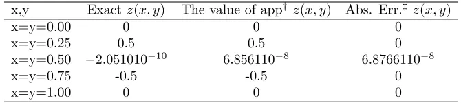
Table 1. Absolute Error ofz(x, y) for different value of x, y.
x,y Exactz(x, y) The value of app† z(x, y) Abs. Err.‡ z(x, y)
x=y=0.00 0 0 0
x=y=0.25 0.5 0.5 0
x=y=0.50 −2.051010−10 6.856110−8 6.8766110−8
x=y=0.75 -0.5 -0.5 0
x=y=1.00 0 0 0
†The value of approximating forz(x, y)
‡Absolute Error forz(x, y)
The exact solution isz(x, y) = sin(πx) cos(πy), so the minimum of the functional is J = 0. According to the proposed method in section 3, we approximate the function z(x, y) in terms of the shifted Legendre polynomial basis with respect to
z(x,0) = sin(πx), z(0, y) =z(1, y) = 0 as following
ˆ
z(x, y)≃
n ∑
i=0
m ∑
j=0
cijxy(x−1)pi(x)pj(y) + sin(πx).
Following those mentioned in section 3, the arbitrary approximation of the function
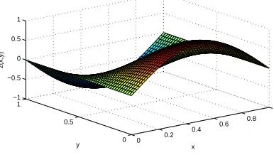
z(x, y) can be found. The validity of this numerical scheme has been analyzed by comparison with the exact solution of the problem. In Figure1, the obtained approx-imate functionz(x, y) by presented method is plotted for n=m = 6. In Figure 2, the approximate solution ofz(x, y) withx= 0.5 and exact solution of the variational problem are plotted together. It is obvious that with increase in the number of the Legendre basis, the approximate values of z(x, y) converge to the exact solution at pointx= 0.5. Furthermore, Table1 reports the approximate value of the function
z(x, y) for different values ofx, y. In this table, the absolute error of the function is reported too. Finally, Table2 presents the value of performance index J at various value ofn, m. We can see that with increase of the number ofn, m, the approximate value ofJ approaches to the exact value of functional, i.e,J = 0.
Table 2. Approximate value of functionalJ∗ for Example5.1.
p.o† n=m=2 n=m=3 n=m=4 n=m=5 n=m=6
J∗ -0.00125768 -0.00125771 −6.256210−7 −6.256210−7 −1.891510−10
†polynomial order
Example 5.2. Consider the following 2D functional
min
z J[z(x, t)] = ∫ 1
0
∫ 1
0
x
2[z
2(x, t) + (∂z(x, t)
∂t )
2]dxdt,
Figure 1. Approximate solution ofz(x, y) forn=m= 6 (Example5.1).
0 0.2
0.4 0.6
0.8 1
0 0.5
1 −1 −0.5 0 0.5 1
x y
z(x,y)
Figure 2. Exact and approximate solution of z(x, y) at x = 0.5
(Example5.1).
0 0.2 0.4 0.6 0.8 1
−1 −0.8 −0.6 −0.4 −0.2 0 0.2 0.4 0.6 0.8 1
y
z(x=0.5,y)
Approximation solution Exact solution
Table 3. Approximate value of functionalJ∗ for Example5.2.
p.o† n=m=2 n=m=3 n=m=4 n=m=5,6
J∗ 0.063466638936 0.063466180052 0.063466179667 0.063466179662
†polynomial order
Applying the Rizt method, the approximate solution of the state functionz(x, t) in terms of the shifted Legendre polynomial basis with respect to z(x,0) = 1−
x2, z(1, t) = 0 is written as
ˆ
z(x, t)≃t.(x−1)
n ∑
i=0
m ∑
j=0
kijpi(x)pj(t) + 1−x2. (5.1)
Figure 3. Approximate solution ofz(x, t) forn=m= 6 (Example5.2).
0 0.2 0.4
0.6 0.8 1 0
0.5 1
0 0.2 0.4 0.6 0.8 1
x t
z(x,t)
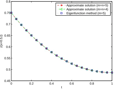
Figure 4. Approximate solution of state functionz(x, t) forx= 0.5 and different value ofm, n(.∗.:m=n= 5,−▹−:m=n= 4) and
..: state function with the eigenfunction method (Example 5.2).
0 0.2 0.4 0.6 0.8 1
0.45 0.5 0.55 0.6 0.65 0.7 0.75 0.8
t
z(x=0.5,t)
Approximate solution (m=n=5) Approximate solution (m=n=4) Eigenfunction method (m=5)
can be considered that the analytical and numerical solutions overlap. We only need a few terms of polynomials to obtain these satisfactory results.
6. Conclusion
In this paper, a numerical solution for a class of variational problems based on Le-gendre polynomials is established. The suggested method reduces the two variables optimization problem to solving an algebraic system of equations. The approximate polynomial function is of good flexibility in the sense of satisfying the initial and boundary conditions in the proposed method. Theoretical analysis was given to sup-port the suggested method. In addition, only a small number of polynomials order are required to obtain a satisfactory result which the given illustrative examples support this claim.
Acknowledgment
The authors are very grateful to two reviewers for their useful comments which improved the quality of the paper.
References
[1] Q. Abdulaziz, I. Hashim and M. S. H. Chowdhury,Solving variational problems by homotopy-perturbation method, Int. J. Numer. Methods Eng.,175(2008), 709-721.
[2] C. Canuto, M. Y. Hussaini, A. Quarteroni and T. A. Zang,Spectral Methods, Fundamentals in Single Domains, Springer- Verlag: Berlin Heidelberg, 2006.
[3] M. Dehghan and M. Tatari,The use of Adomian decomposition method for solving problems in calculus of variation, Math. Prob. Eng.,2006(2006), 1-12.
[4] R. Y. Chang and M. L. Wang, Shifted Legendre direct method for variational problems, J. Optimi. Theory Appl.,39(1983), 299-307.
[5] C. F. Chen and C. H. Hsiao,A Walsh series direct method for solving variational problem, J. Franklin Instit.,300(1975),265-280.
[6] l. E. Elgolic,Calculus of Variations, Pergamon press, Oxford, 1962.
[7] L. Elsgolts,Differential Equations and the Calculus of Variations, translated from the Russian by G. Yankovsky, Mir Publisher, Moscow. 1977.
[8] I. M. Gelfand and S. V. Fomin, Calculus of Variations, Prentice-Hall, Englewood Cliffs, NJ. 1963.
[9] W. Glabisz,Direct Walsh-wavelet packet method for variational problems, Appl. Math. Com-put.,159(2004), 769-781.
[10] I. R. Horng and J. H. Chou,Shifted Chebyshev direct method for solving variational problems, Int. J. Syst. Sci.,16(1985), 855-861.
[11] C. H. Hsiao,Haar wavelet direct method for solving variational problems, Math. Comput. Simul.,
64(2004), 569-585.
[12] C. Hwang and Y. P. Shih, Laguerre series direct method for variational problems, J. Optim. Theory Appl.,39(1983), 143-149.
[13] E. Kreyszig,Introductory Functional Aanalysis with Applications, John Wiley and Sons Inc., 1978.
[14] L. P. Lebedev and M. J. Cloud, The Calculus of Variations and Functional Analysis With Optimal Control and Applications in Mechanics, World Scientific Publishing Co. Pte. Ltd., 2003.
[16] N. ¨Ozdemir, O. P. Agrawal, D. Karadeniz, and B. B. Iskender, Fractional optimal control problem of an axis-symmetric diffusion-wave propagation, Physica Scripta,T136(2009), 014024. [17] M. Razzaghi and Y. Ordokhani,An application of rationalized Haar functions for variational
problems, Appl. Math. Comput.,122(2001), 353-364.
[18] M. Razzaghi and M. Razzaghi,Fourier series direct method for variational problems, Int. J. Control,48(1988), 887-895.
[19] M. Razzaghi and S. A. Yousefi,Legendre wavelets direct method for variational problems, Math. Comput. Simul.,53(2000), 185-192.
[20] H. L. Royden,Real Analysis, 3rd Ed, Macmillan Publishing Company, U.S.A. 1988.
[21] M. Stone,The Generalized Weierstrass Approximation Theorem, Mathematics Magazine,21, N.21(1948), 167-184 and21, N.5(1948), 237-254.
[22] M. Tatari and M. Dehghan,Solution of problems in calculus of variations via He’s variational iteration method, Phys. Lett. A,362(2007), 401-406.
[23] V. M. Tikhomirov,Store about Maxima and Minima, American Mathematica Society, Provi-dence, RI, 1990.
[24] S. A. Yousefi and M. Dehghan,The use of He’s variational iteration method for solving varia-tional problems, International Journal of Computer Mathematics,87(2010), 1299-1314. [25] S. A. Yousefi, D. Lesnic and Z. Barikbin,Satisfier function in Ritz-Galerkin method for the