Estuarine Dynamics as a Function of Barrier Island Transgression and Wetland Loss: Understanding the Transport and Exchange Processes

(1)

University of New Orleans University of New Orleans

ScholarWorks@UNO

University of New Orleans Theses and

Dissertations Dissertations and Theses

12-17-2010

Estuarine Dynamics as a Function of Barrier Island Transgression

and Wetland Loss: Understanding the Transport and Exchange

Processes

Jennifer Schindler University of New Orleans

Follow this and additional works at: https://scholarworks.uno.edu/td

Recommended Citation Recommended Citation

Schindler, Jennifer, "Estuarine Dynamics as a Function of Barrier Island Transgression and Wetland Loss: Understanding the Transport and Exchange Processes" (2010). University of New Orleans Theses and Dissertations. 1260.

https://scholarworks.uno.edu/td/1260

This Thesis is protected by copyright and/or related rights. It has been brought to you by ScholarWorks@UNO with permission from the rights-holder(s). You are free to use this Thesis in any way that is permitted by the copyright and related rights legislation that applies to your use. For other uses you need to obtain permission from the rights-holder(s) directly, unless additional rights are indicated by a Creative Commons license in the record and/or on the work itself.

(2)

Estuarine Dynamics as a Function of Barrier Island Transgression and Wetland Loss: Understanding the Transport and Exchange Processes

A Thesis

Submitted to the Graduate Faculty of the University of New Orleans

in partial fulfillment of the requirements for the degree of

Master of Science in

Earth and Environmental Science Coastal Sciences

by

Jennifer Schindler

B.S. University of New Orleans, 2008

(3)

ii

(4)

iii

ACKNOWLEDGMENTS

I consider this master’s thesis to be a major accomplishment in my life. Therefore, I owe my deepest gratitude to all those who have made this thesis a possibility. First, I would like to thank my major professor, Dr. Ioannis Georgiou, who has taught me most of what I know about numerical modeling while working for him over the last 4 years. This research would not have been possible if it were not for his guidance and support. On a similar note, I would like to thank my committee members, Dr. Mark Kulp and Dr. Alex McCorquodale for their expertise and advice not just during this research, but throughout my undergraduate and graduate career as well. The field data used in this research would not exist if it were not for the people responsible for the field deployments and retrievals: Mike Brown, Chris Esposito, Dr. Ioannis Georgiou, Phil McCarty, Kevin Trosclair, and Dallon Weathers. Funding provided by the USGS Northern Gulf of Mexico (NGOM) Ecosystem Change and Hazard Susceptibility Project made field efforts and research work possible. Therefore, I would like to thank this organization for its generosity and support. To my friends, family,

(5)

iv

LIST OF FIGURES

Figure 1 – The inset shows a map of the states surrounding the northern Gulf of Mexico, while the red box outlines the area shown in the large image. The large image is a relief map of the region surrounding the northern Gulf of Mexico (the study area) with water

bodies and rivers labeled. ... 1

Figure 2 - The Penland Model of transgressive depositional systems describes three stages of geomorphology including Stage 1 with erosional flanking barriers, Stage 2 with a transgressive barrier island arc, and Stage 3 with a transformation to inner-shelf shoals (Penland, Boyd, and Suter, 1988). ... 3

Figure 3 - A map of the six delta complexes within the Holocene MDP. The two active complexes are the Atchafalaya and Modern (Balize) complex (Frazier, 1967). ... 6

Figure 4 - Map of the upper and central Pontchartrain Estuary. River names are shown in italics. (Figure adapted from Georgiou et al., 2009.) ... 7

Figure 5 - Principal hydrodynamic features within Barataria Basin (Georgiou et al., 2010). ... 8

Figure 6 - Estuarine salinity gradients as a function of longitude; error bars represent one standard deviation (Georgiou et al., 2009). ... 9

Figure 7 - The inset shows a map of the states surrounding the northern Gulf of Mexico, while the box outlines the area shown in the large image. The large image is a map of southeast Louisiana showing the regional bathymetry (meters) and coastline features as well as the location of the Chandeleur Islands (Georgiou and Schindler, 2009). Red circles indicate deployment locations (D1 and D2). ... 12

Figure 8 - Map of tidal exchange transects. Contours show the wet/dry parameter for the base-case scenario. (Zero represents subaerial elements, gray represents water elements.)... 16

Figure 9 - Schematic diagram of variables used in the definition of the energy equation. ... 17

Figure 10 -Entire computational grid domain mesh from southeast Louisiana to the Florida/Alabama state line (coordinates in UTM 15, meters). ... 20

Figure 11 - Entire computational grid domain from southeast Louisiana to the Florida/Alabama state line (coordinates in UTM 15, meters). Bathymetric contours are shown with depth in meters. ... 21

Figure 12 - Northwestern area of domain including Lakes Pontchartrain, Maurepas, and Borgne as well as connecting channels such as the IHNC, Rigolets, MRGO, and ICWW: (Top) Domain mesh and (Bottom) Base-case bathymetric contours with depth shown in meters. ... 22

Figure 13 - Southeastern area of domain including the Biloxi Marsh, Chandeleur Islands and Sound, Mississippi barrier islands and Sound, MRGO, and Lake Borgne: (Top) Domain mesh and (Bottom) Base-case bathymetric contours with depth shown in meters. ... 23

Figure 14 - Base-case contour plot of water depth in meters. ... 25

Figure 15 – H1 contour plot of water depth in meters. ... 25

(8)

vii

Figure 17 - The inset shows a map of the states surrounding the northern Gulf of Mexico, while the red box outlines the area shown in the large image. The large image is a map of the calibration stations within the domain. Table 3 describes these stations in more

detail. ... 29 Figure 18 - Meteorological conditions at the NOAA NOS Gulfport Outer Range station

(Station GPOM6 – 8744707) for the period of 3/31/10 to 5/7/10. ... 30 Figure 19 – Comparison of base-case scenario tides (meters) and observed tide data for the

calibration period (3/31/10 to 4/22/10). Calibration efforts focused on good correlation during the period of 4/16/10 to 4/22/10 (inside the green box) at the following locations (from top to bottom): Lake Pontchartrain at LUMCON, Rigolets near Lake Pontchartrain, and Mississippi Sound at St. Joseph Island Light. An adjustment

was applied to observed data to account for vertical datum differences... 31 Figure 20 - Comparison of base-case scenario tides (meters) and observed tide data for the

calibration period (3/31/10 to 4/22/10). Calibration efforts focused on good correlation during the period of 4/16/10 to 4/22/10 (inside the green box) at the locations (from top to bottom): D2, NE Bay Gardene near Point à la Hache and Barataria Pass at Grand Isle. An adjustment was applied to observed data to account

for vertical datum differences. ... 32 Figure 21 - Comparison of base-case scenario salinities (ppt) and observed salinity data for

the calibration period (3/31/10 to 4/22/10). Calibration efforts focused on good correlation during the period of 4/16/10 to 4/22/10 (inside the green box) at the locations (from top to bottom) Rigolets near Lake Pontchartrain, Mississippi Sound at St. Joseph Light, and NE Bay Gardene near Point à la Hache. An adjustment was applied

to observed data to account for sensor height differences. ... 33 Figure 22 – A comparison of the tidal elevations (in meters) across the model scenarios

(Base-case, H1, and H2) at Lake Pontchartrain LUMCON(top) and Rigolets (bottom) for the entire simulation period. The winter storm period of 4/22/10 through 5/7/10 is

bounded by the purple box. ... 36 Figure 23 - A comparison of the tidal elevations (in meters) across the model scenarios

(base-case, H1, and H2) at the Mississippi Sound at St. Joseph Island Light (top) and D2 (bottom) stations for the entire simulation period. The winter storm period of

4/22/10 through 5/7/10 is bounded by the purple box. ... 37 Figure 24 - A comparison of the tidal elevations (in meters) across the model scenarios

(base-case, H1, and H2) at the NE Bay Gardene station for the entire simulation period.

The winter storm period of 4/22/10 through 5/7/10 is bounded by the purple box. ... 38 Figure 25 - A comparison of the tidal elevations (in meters) across the model scenarios

(base-case, H1, and H2) at the Grand Isle station for the entire simulation period. The

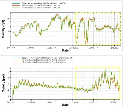
winter storm period of 4/22/10 through 5/7/10 is bounded by the purple box. ... 38 Figure 26 - A comparison of the salinity fluctuations (in ppt) across the model scenarios

(base-case, H1, and H2) at Lake Pontchartrain LUMCON (top) and Rigolets (bottom) for the entire simulation period. The winter storm period of 4/22/10 through 5/7/10 is

bounded by the yellow box. ... 39 Figure 27 - A comparison of the salinity fluctuations (in ppt) across the model scenarios

(9)

viii

the entire simulation period. The winter storm period of 4/22/10 through 5/7/10 is

bounded by the yellow box. ... 40 Figure 28 - A comparison of the salinity fluctuations (in ppt) across the model scenarios

(base-case, H1, and H2) at the D2 for the entire simulation period. The winter storm

period of 4/22/10 through 5/7/10 is bounded by the yellow box. ... 40 Figure 29 - A comparison of the salinity fluctuations (in ppt) across the model scenarios

(base-case, H1, and H2) at the NE Bay Gardene station for the entire simulation period.

The winter storm period of 4/22/10 through 5/7/10 is bounded by the yellow box. ... 41 Figure 30 - A comparison of the salinity fluctuations (in ppt) across the model scenarios

(base-case, H1, and H2) at the Grand Isle station for the entire simulation period. The

winter storm period of 4/22/10 through 5/7/10 is bounded by the yellow box. ... 41 Figure 31 – Contour plot (time and space variant) of Bayou La Loutre cross-shore flux in

m3_{/s during the three simulation scenarios: (a) Base-case, (b) H1, and (c) H2. Distance}

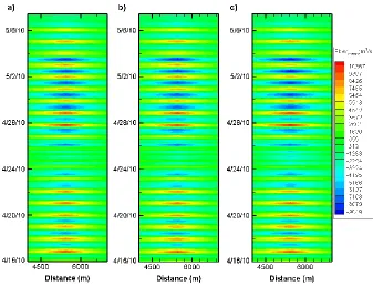
is from north to south. ... 44 Figure 32 - Contour plot (time and space variant) of the Rigolets transect’s cross-shore flux

in m3_{/s during the three simulation scenarios: (a) Base-case, (b) H1, and (c) H2.}

Distance is from north to south. ... 44 Figure 33 - Contour plot (time and space variant) of Cat Island cross-shore flux in m3_/s

during the three simulation scenarios: (a) Base-case, (b) H1, and (c) H2. Distance is

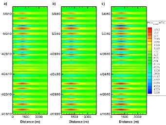
from north to south. ... 45 Figure 34 - Contour plot (time and space variant) of the primary Cat Island channel

cross-shore flux in m3_{/s from distance 4,000 to 7,000 m from north to south during the three}

simulation scenarios: (a) Base-case, (b) H1, and (c) H2. Distance is from north to south. ... 45 Figure 35 - Contour plot (time and space variant) of Half Moon Island cross-shore flux in

m3_{/s during the three simulation scenarios: (a) Base-case, (b) H1, and (c) H2. Distance}

is from north to south. ... 46 Figure 36 - Contour plot (time and space variant) of the primary Half Moon Island channel

cross-shore flux in m3_{/s from distance 0 to 4,000 m from north to south during the} three simulation scenarios: (a) Base-case, (b) H1, and (c) H2. Distance is from north to

south. ... 46 Figure 37 - Contour plot (time and space variant) of the Chandeleur Island transect’s

cross-shore flux in m3_{/s during the three simulation scenarios: (a) Base-case, (b) H1, and (c)}

H2. Distance is from north to south. ... 47 Figure 38 - Contour plot (time and space variant) of the primary Chandeleur Island

transect’s cross-shore flux in m3_{/s from distance 66,000 to 96,000 m from north to} south during the three simulation scenarios: (a) Base-case, (b) H1, and (c) H2. Distance

is from north to south. ... 47 Figure 39 - Contour plot (time and space variant) of the Ship Island to Hewes Point

transect’s cross-shore flux in m3_{/s during the three simulation scenarios: (a) Base-case,}

(b) H1, and (c) H2. Distance is from north to south. ... 48 Figure 40 – Instantaneous flow (m3_{/s) across the Chef Menteur transect during the three}

(10)

ix

Figure 41 - Instantaneous flow (m3_{/s) across the ICWW transect during the three}

simulation scenarios: Base-case, H1, and H2. ... 49 Figure 42 – H1 instantaneous flow (m3_{/s) across the domain during the normal period. The}

domain was divided into sections referred to as the upper, middle, lower-middle, and

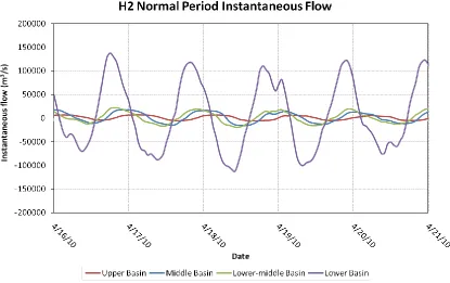
lower basin. ... 50 Figure 43 – H2 instantaneous flow (m3_{/s) across the domain during the normal period. The}

domain was divided into sections referred to as the upper, middle, lower-middle, and

lower basin. ... 50 Figure 44 – H1 instantaneous flow (m3_{/s) across the domain during the winter storm}

period. The domain was divided into sections referred to as the upper, middle,

lower-middle, and lower basin. ... 51 Figure 45 – H2 instantaneous flow (m3_{/s) across the domain during the winter storm}

period. The domain was divided into sections referred to as the upper, middle,

lower-middle, and lower basin. ... 51 Figure 46 - Average difference in tides (m) between the base-case and H1 scenarios. Tides

were averaged over the entire simulation period. ... 52 Figure 47 - Average difference in tides (m) between the base-case and H2 scenarios. Tides

were averaged over the entire simulation period. ... 52 Figure 48 - Average difference in salinity between the base-case and H1 scenarios (salinity

in ppt). Salinity was averaged over the entire simulation period. ... 53 Figure 49- Average difference in salinity between the base-case and H2 scenarios (salinity

in ppt). Salinity was averaged over the entire simulation period. ... 53 Figure 50 – Base-case water elevation as well as depth-averaged current velocity and

magnitude on 4/25/10; winds are 15 m/s from the west/southwest. The velocity vectors orientation indicates the direction the current is moving. The length of the vector indicates the current magnitude (see upper right corner of figure for reference

vector). Color contours represent water elevation above mean sea level. ... 54 Figure 51 – H2 water elevation as well as depth-averaged current velocity and magnitude

on April 25, 2010; winds are 15 m/s from the west/southwest. The velocity vectors orientation indicates the direction the current is moving. The length of the vector indicates the current magnitude (see upper right corner of figure for reference vector).

Color contours represent water elevation above mean sea level. ... 55 Figure 52 - Circulation patterns based on flow dominance specified in Table 6 and Table 7.

The left panel shows circulation patterns for the normal period while the right panel shows winter storm circulation patterns. The base-case, H1, and H2 circulation

patterns are shown in top, middle, and bottom panels, respectively. Contours show the wet/dry parameter for the base-case scenario (zero represents subaerial elements, gray represents water elements). An arrow to the right represents ebb-dominant flow

conditions. ... 56 Figure 53 – Bathymetric contours of the Barataria Basin and Mississippi River delta. (UTM

15 coordinates and bathymetries in meters) ... 64 Figure 54 – Mesh of the Barataria Basin and Mississippi River delta (UTM 15 coordinates in

(11)

x

Figure 55– Detailed view of the Barataria Basin mesh. (UTM 15 coordinates in meters) ... 65 Figure 56– Detailed view of the Bay St. Louis mesh and bathymetric contours. (UTM 15

coordinates and bathymetries in meters) ... 65 Figure 57 – Mesh of Biloxi Bay including Ship Island and Horn Island. (UTM 15 coordinates

in meters) ... 66 Figure 58 – Mesh of the Mississippi Sound including Biloxi Bay, Cat Island, Ship Island, and

Horn Island. (UTM 15 coordinates in meters) ... 66 Figure 59 - Detailed view of the Chandeleur and Breton Sound mesh including the

Chandeleur Islands, Biloxi Marsh, Bayou La Loutre, and Breton Island. (UTM 15

coordinates in meters) ... 67 Figure 60- Detailed view of the Chandeleur and Breton Sound mesh, including the

Chandeleur Islands, Biloxi Marsh, Bayou La Loutre, and Breton Island, with

bathymetric contours. (UTM 15 coordinates and bathymetries in meters) ... 67 Figure 61– Bathymetric contours of the eastern Pontchartrain Estuary including Lake

Pontchartrain, Lake Borgne, and major channels such as the Rigolets, IHNC, ICWW, and

MRGO. (UTM 15 coordinates and bathymetries in meters) ... 68 Figure 62 – Mesh of the eastern Pontchartrain Estuary including Lake Pontchartrain, Lake

Borgne, and major channels such as the Rigolets, IHNC, ICWW, and MRGO. (UTM 15

coordinates and bathymetries in meters) ... 68 Figure 63 – Bathymetric contours of the Mobile Bay including Dauphin Island and the

Mobile Bay Ship Channel. (UTM 15 coordinates and bathymetries in meters) ... 69 Figure 64– Detailed view of the mesh and bathymetric contours of the Mobile Bay including

Dauphin Island and the Mobile Bay Ship Channel. (UTM 15 coordinates and

bathymetries in meters) ... 69 Figure 65 – Bathymetric contours of the Mississippi River Delta. (UTM 15 coordinates and

bathymetries in meters) ... 70 Figure 66 – Mesh of the Mississippi River Delta. (UTM 15 coordinates in meters) ... 70 Figure 67 - Comparison of base-case scenario tides (meters) and observed tide data for the

calibration period (3/31/10 to 4/22/2010). Calibration efforts focused on good correlation during the period of 4/16/10 to 4/22/10 at the Bay Waveland Yacht Club station. An adjustment was applied to observed data to account for vertical datum

differences. ... 71 Figure 68 - Comparison of base-case scenario tides (meters) and observed tide data for the

calibration period (3/31/10 to 4/22/2010). Calibration efforts focused on good correlation during the period of 4/16/10 to 4/22/10 at the Chef Menteur Pass near Lake Borgne station. An adjustment was applied to observed data to account for

vertical datum differences. ... 71 Figure 69 - Comparison of base-case scenario tides (meters) and observed tide data for the

calibration period (3/31/10 to 4/22/2010). Calibration efforts focused on good correlation during the period of 4/16/10 to 4/22/10 at the D1 location. An adjustment

was applied to observed data to account for vertical datum differences... 71 Figure 70 - Comparison of base-case scenario tides (meters) and observed tide data for the

(12)

xi

correlation during the period of 4/16/10 to 4/22/10 at the IHNC, New Orleans station.

An adjustment was applied to observed data to account for vertical datum differences. ... 72 Figure 71 - Comparison of base-case scenario tides (meters) and observed tide data for the

calibration period (3/31/10 to 4/22/2010). Calibration efforts focused on good correlation during the period of 4/16/10 to 4/22/10 at the Mississippi Sound at Grand Pass station. An adjustment was applied to observed data to account for vertical datum

calibration period (3/31/10 to 4/22/2010). Calibration efforts focused on good correlation during the period of 4/16/10 to 4/22/10 at the Pass Manchac station. An

adjustment was applied to observed data to account for vertical datum differences. ... 72 Figure 73 - Comparison of base-case scenario tides (meters) and observed tide data for the

calibration period (3/31/10 to 4/22/2010). Calibration efforts focused on good correlation during the period of 4/16/10 to 4/22/10 at the Shell Beach, Louisiana, station. An adjustment was applied to observed data to account for vertical datum

calibration period (3/31/10 to 4/22/2010). Calibration efforts focused on good correlation during the period of 4/16/10 to 4/22/10 at the Pilots Station East, SW Pass, Louisiana, station. An adjustment was applied to observed data to account for

vertical datum differences. ... 73 Figure 75 - Comparison of base-case scenario salinities (ppt) and observed salinity data for

the calibration period (3/31/10 to 4/22/2010). Calibration efforts focused on good correlation during the period of 4/16/10 to 4/22/10 at the D1 station. An adjustment

was applied to observed data to account for sensor height differences. ... 73 Figure 76 - Comparison of base-case scenario salinities (ppt) and observed salinity data for

the calibration period (3/31/10 to 4/22/2010). Calibration efforts focused on good correlation during the period of 4/16/10 to 4/22/10 at the D2 station. An adjustment

was applied to observed data to account for sensor height differences. ... 74 Figure 77 - Comparison of base-case scenario salinities (ppt) and observed salinity data for

the calibration period (3/31/10 to 4/22/2010). Calibration efforts focused on good correlation during the period of 4/16/10 to 4/22/10 at the Mississippi Sound at Grand Pass station. An adjustment was applied to observed data to account for sensor height

differences. ... 74 Figure 78 - Comparison of base-case scenario salinities (ppt) and observed salinity data for

the calibration period (3/31/10 to 4/22/2010). Calibration efforts focused on good correlation during the period of 4/16/10 to 4/22/10 at the Lake Pontchartrain LUMCON station. An adjustment was applied to observed data to account for sensor

height differences. ... 74 Figure 79 - A comparison of the tidal elevations (in meters) across the model scenarios

(base-case, H1, and H2) at the SW Pass station for the entire simulation period. The

winter storm period of 4/22/10 through 5/7/10 is bounded by the purple box. ... 75 Figure 80 - A comparison of the tidal elevations (in meters) across the model scenarios

(13)

xii

simulation period. The winter storm period of 4/22/10 through 5/7/10 is bounded by

the purple box. ... 75 Figure 81- A comparison of the tidal elevations (in meters) across the model scenarios

(base-case, H1, and H2) at the Chef Menteur Pass station for the entire simulation period. The winter storm period of 4/22/10 through 5/7/10 is bounded by the purple

box. ... 75 Figure 82- A comparison of the tidal elevations (in meters) across the model scenarios

(base-case, H1, and H2) at the D1 station for the entire simulation period. The winter

storm period of 4/22/10 through 5/7/10 is bounded by the purple box. ... 76 Figure 83- A comparison of the tidal elevations (in meters) across the model scenarios

(base-case, H1, and H2) at the Mississippi Sound at Grand Pass station for the entire simulation period. The winter storm period of 4/22/10 through 5/7/10 is bounded by

the purple box. ... 76 Figure 84- A comparison of the tidal elevations (in meters) across the model scenarios

(base-case, H1, and H2) at the Pass Manchac station for the entire simulation period.

The winter storm period of 4/22/10 through 5/7/10 is bounded by the purple box. ... 76 Figure 85 - A comparison of the salinity fluctuations (in ppt) across the model scenarios

(base-case, H1, and H2) at the SW Pass station for the entire simulation period. The

winter storm period of 4/22/10 through 5/7/10 is bounded by the yellow box. ... 77 Figure 86 - A comparison of the salinity fluctuations (in ppt) across the model scenarios

(base-case, H1, and H2) at the Bay Waveland Yacht Club station for the entire

simulation period. The winter storm period of 4/22/10 through 5/7/10 is bounded by

the yellow box. ... 77 Figure 87 - A comparison of the salinity fluctuations (in ppt) across the model scenarios

(base-case, H1, and H2) at the Chef Menteur Pass station for the entire simulation period. The winter storm period of 4/22/10 through 5/7/10 is bounded by the yellow

box. ... 77 Figure 88 - A comparison of the salinity fluctuations (in ppt) across the model scenarios

(base-case, H1, and H2) at the D1 station for the entire simulation period. The winter

storm period of 4/22/10 through 5/7/10 is bounded by the yellow box. ... 78 Figure 89 - A comparison of the salinity fluctuations (in ppt) across the model scenarios

(base-case, H1, and H2) at the IHNC station for the entire simulation period. The

winter storm period of 4/22/10 through 5/7/10 is bounded by the yellow box. ... 78 Figure 90 - A comparison of the salinity fluctuations (in ppt) across the model scenarios

(base-case, H1, and H2) at the Mississippi Sound at Grand Pass station for the entire simulation period. The winter storm period of 4/22/10 through 5/7/10 is bounded by

the yellow box. ... 78 Figure 91 - A comparison of the salinity fluctuations (in ppt) across the model scenarios

(base-case, H1, and H2) at the Pass Manchac station for the entire simulation period.

The winter storm period of 4/22/10 through 5/7/10 is bounded by the yellow box. ... 79 Figure 92 - A comparison of the salinity fluctuations (in ppt) across the model scenarios

(base-case, H1, and H2) at the Shell Beach station for the entire simulation period. The

(14)

xiii

LIST OF TABLES

Table 1 - Simulation table describing the simulation name, objective, computational grid

details, and analysis methods used. ... 15 Table 2 - Transect number, name, and number of equidistant points corresponding with

Figure 8. ... 16 Table 3 - Stations used for model calibration. Station name, number, and operating agency,

as well as calibration parameter are provided. Station numbers are in parentheses

after station name... 29 Table 4 – MAE and RMSE values (in meters) at each tidal calibration station during the

period of 4/16/10 to 4/22/10. Stations are shown in ascending order of error. ... 34 Table 5 - MAE and RMSE values (in ppt) at each salinity calibration station during the

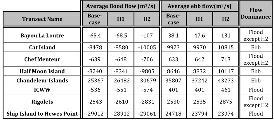
period of 4/16/10 to 4/22/10. Stations are shown in ascending order of error. ... 35 Table 6 - Average flood and ebb flows (m3_{/s) through each transect during normal}

conditions (April 16 through April 21)... 42 Table 7 - Average flood and ebb flows (m3_{/s) through each transect during winter storm}

conditions (April 22 through May 7). ... 42 Table 8 – Comparison of the normal period and the winter storm period (Table 6 and Table

7) in terms of percent change in flow through each transect. Negative percentages

(15)

xiv

ABSTRACT

The Northern Gulf of Mexico and coastal Louisiana are experiencing accelerated relative sea level rise rates; therefore, the region is ideal for modeling the global affects of sea level rise (SLR) on estuarine dynamics in a transgressive barrier island setting. The field methods and numerical modeling in this study show that as barrier islands are converted to inner shoals, tidal exchange increases between the estuary and coastal ocean. If marshes are unable to accrete at a pace comparable to SLR, wetlands will deteriorate and the tidal exchange and tidal prism will further increase. Secondary to hurricanes, winter storms are a primary driver in coastal morphology in this region, and this study shows that wind direction and magnitude, as well as atmospheric pressure change greatly affect estuarine exchange. Significant wetland loss and winter storm events produce changes in local and regional circulation patterns, thereby affecting the hydrodynamic exchange and resulting transport.

(16)

1

CHAPTER 1

Introduction

On low gradient continental shelves around the world, including the northern Gulf of Mexico (Figure 1), the abandonment of an active delta lobe due to upstream avulsion and reduced sediment supply leads to barrier island development across interdistributary bays (Penland, Boyd, and Suter, 1988; Roberts, 1997). These processes follow a conceptual model described by Penland, Boyd, and Suter (1988). This three-stage model explains how deltaic headlands submerge and sediment is reworked by marine processes, eventually forming barrier islands. As these processes continue, eroding headlands produce spit systems and breaching events generate inlets. Tidal inlets control the exchange between the coastal ocean and interior bays and sounds; therefore, they strongly influence the evolution of barrier islands. An increase in the size of tidal inlets causes an increase in the tidal prism, or volume of water passing through the tidal inlet (O'Brien, 1969; Jarrett, 1976; Hughes, 2002). After continued transgression due to longshore and cross-shore transport and with effects from rising sea levels, only inner-shelf shoals will remain. Marine processes cause these subaqueous sand bodies to slowly migrate landward (Penland, Boyd, and Suter, 1988; Roberts, 1997).

Figure 1 – The inset shows a map of the states surrounding the northern Gulf of Mexico, while the red box outlines the area shown in the large image. The large image is a relief map of the region

surrounding the northern Gulf of Mexico (the study area) with water bodies and rivers labeled.

(17)

2

2005). These factors directly determine wetland loss or gain, tidal exchange, and the bay tidal prism (Georgiou et al., 2010; FitzGerald et al., 2008). Presently, the Chandeleur Island arc, created when the Mississippi River abandoned the St. Bernard Delta complex, is fragmented with

subaqueous shoals at both ends of the barrier island arc. The impact of major storms and the asymmetry in longshore transport along the islands (Georgiou and Schindler, 2009) will likely accelerate this process until, in the absence of an active littoral zone, cross-shore transport begins to dominate (Miner et al., 2009; Twichell et al., 2009).

Therefore, the Chandeleur Islands serve as a model for transgressive barrier islands having a limited supply of sand along storm-dominated coasts. Recent studies (Sallenger et al., 2009) show that the Chandeleur Islands have lost 86% of their subaerial exposure during Hurricane Katrina in 2005, and an additional 20% during winter, extra-tropical, and tropical storms in the three years following hurricane Katrina. Therefore, this system provides a unique opportunity to study the estuarine dynamics during this transitional stage from barrier arc to segmented sandy shoals in a regime of accelerated sea-level-rise (SLR) and increased storminess(Goldenberg et al., 2001; Emanuel, 2005; Blum and Roberts, 2009).

Two key objectives of this research were to obtain physical measurements from the interior bay or sound landward of the Chandeleur Islands and to investigate (through numerical modeling) exchange processes during moderate-energy conditions, such as those produced by winter storms. These storms are important to the region’s morphology, as they have a higher frequency of

occurrence than tropical storms and hurricanes. There are at least 20 to 40 winter storms each year in this area (Georgiou, FitzGerald, and Stone, 2005).

The key research questions included the following: (1) During barrier fragmentation, to what degree will the exchange between the coastal ocean and back-barrier basins influence the transport and mixing processes of conservative and dissolved substances; (2) Does an increase in the tidal exchange along barrier systems increase marine conditions in interior bays; (3) How does the astronomical forcing and spring neap variation influence tidal transport in back basins; and (4) How do estuarine dynamics in the bays respond to north/northwesterly wind direction, longer wind duration, and higher wind intensity during winter storms?

Background and Significance

Roberts (1997) describes the delta cycle as consisting of two phases: a regressive phase and a transgressive phase. Delta lobes are formed as streams capture sediment from runoff and well-defined river channels deliver sediment to wetlands and bays. Since the river has many

distributaries and avulsions that vary with time, there can be many delta lobes per delta complex. Eventually the river will switch course and begin a new delta complex, starving the first delta complex of sediment input. The abandoned delta complex will subside due to compaction and deteriorate due to marine processes. This transgressive reworking forms beaches, spits, barrier islands, and, finally, subaqueous shoals. In this way, the Mississippi River has built the wetlands, bayous, barrier islands, natural levees, and tidal channels of the Mississippi Delta Plain.

(18)

3

The Chandeleur Island chain, as the oldest subaerial transgressive barrier island arc in the Mississippi River delta plain, has been an important feature in the southeastern Louisiana topography. Barrier islands form the first line of defense in protecting coastal wetlands and

shorelines from the direct effects of wind, waves, and storm surge, especially during tropical events (Stone and McBride, 1998; Stone, Zhang, and Sheremet, 2005). Additionally, barrier islands aid in the establishment of estuarine gradients (Reyes et al., 2005). Therefore, these features create a transition zone between marine and freshwater environments, as well as offer subaerial nesting habitat for shorebirds, shallow habitat nurseries for marine life, and spawning grounds for fisheries (Reyes et al., 2005; van Heerden and DeRouen, 1997).

Figure 2 - The Penland Model of transgressive depositional systems describes three stages of geomorphology including Stage 1 with erosional flanking barriers, Stage 2 with a transgressive barrier island arc, and Stage 3 with a transformation to inner-shelf shoals (Penland, Boyd, and Suter, 1988).

(19)

4

Understanding the relationship between barrier island fragmentation and tidal prism, therefore, is imperative in predicting changes to the interior wetlands and coastline.

Miner et al. (2009) state that the drastic and unpredictable nature of changes in tidal inlets results from “complex bathymetry and resulting wave refraction patterns, as well as increased wave-generated and tidal current-induced sediment transport.” While there has been little research previously conducted to study the effect of barrier island fragmentation (and therefore tidal inlet formation) on estuarine exchange (FitzGerald et al., 2007; FitzGerald et al., 2008; Feng, 2009; Feng and Li, 2010), there have been numerous studies that attempt to define a relationship between an area’s tidal prism and tidal inlet cross-sectional area (O'Brien, 1969; Jarrett, 1976; Hughes, 2002).

Most recently, D' Alpaos et al. (2010) tested the applicability of such an empirical relationship for sheltered inlets:

(Eqn. 1)

where Ω is the cross-sectional area of the tidal inlet in m2_{, P is the tidal prism in m}3_{, and α typically} ranges from 0.85 to 1.10 (O'Brien, 1969; Jarrett, 1976; Hughes, 2002). Using one-dimensional numerical modeling, D' Alpaos et al. (2010) found that a value of k = 1.3 x 10-3_m2-3α _{and α = 0.67 (as} originally derived empirically by O’Brien (1969) and theoretically by Marchi (1990)) produced results concurrent with observational data. Deemed accurate by D' Alpaos et al. (2010), the Marchi Law (Marchi, 1990) relates k to the channel width:

_{(Eqn. 2)}

where B is the channel width in meters. These theoretical relationships, however, may not apply to inlets on open coasts (D' Alpaos et al., 2010), due in part to the effects of longshore transport , sediment transport due to direct and intense wave attack, and wetting and drying of neighboring marshes. Additionally, D' Alpaos et al. (2010) proved that for larger tidal inlets and prisms, α = 0.67 is more appropriate in Equation 1. For tidal inlet cross-sectional areas less than 50 m2 _and/or_tidal prisms less than 106 m3, the tidal prism changes at a much faster rate than the tidal inlet cross-sectional area.

In a report by Jarrett (1976), data were used to establish a regression equation for Gulf of Mexico tidal inlets with and without jetties. The data used displayed more scatter than in other regions such as the east coast (Jarrett, 1976), and therefore the regression equation may not be entirely accurate. Jarrett (1976) proposes that this scatter is the result of the Gulf of Mexico’s microtidal environment, which varies from diurnal to semi-diurnal depending on geographic location and declination of the moon. To reduce uncertainty, tidal inlet cross-sectional areas used to establish this equation were measured during diurnal tide conditions, since the inlet cross-sectional areas in the Gulf coast region are largely influenced by prior astronomical and/or

meteorological effects (Jarrett, 1976). For unjettied or single-jettied inlets along the Gulf Coast, this relationship is:

_{(Eqn. 3)}

where A is the minimum cross-section of the entrance channel measured below mean sea level (ft2₎ and V is the tidal prism corresponding to the diurnal or spring range of tide (ft3_).

(20)

5

intensify landward of the islands per unit length along a cross-shore profile, increases (Georgiou and Schindler, 2009). Both astronomical and meteorological effects influence this exchange. Studies show that winds along the long axis of the Chandeleur/Breton Sound cause extensive setup (~0.2 m with 9 m/s wind speeds) along the downwind coast, but currents and water levels rapidly normalize within three hours when the wind stops (Hart and Murray, 1978). During cold front conditions, waves are fetch-limited within the sounds and depth-limited over shoals and near islands (Keen, 2002). These dynamic conditions can provide additional controls and ultimately further increase the exchange between the coastal ocean and interior bays and sounds.

Relationships that describe the morphological changes anticipated with variations in tidal prism or tidal inlet cross-sectional area can be applied to better understand the effects of sea level rise on barrier islands, interior wetlands, and back-basins (FitzGerald et al., 2008). If marshes are unable to accrete at the same rate as SLR, wetlands will convert to open water under the effects of SLR. This transition will increase the tidal exchange, thereby increasing tidal prism (FitzGerald et al., 2008). Moreover, shoreline change analysis as a function of recent tropical storm activity predicts (through extrapolation) that if the current storm activity persists, the shoreline along the barrier arc would intercept the edge of the back-barrier marsh of the Chandeleur Islands, and could vanish as soon as 2013 (Fearnley et al., 2009). This back-barrier stabilizes the islands by

promoting sediment accumulation and reducing wave energy (FitzGerald et al., 2008; Lavoie et al., 2009). Therefore, the Chandeleur Islands in the northern Gulf of Mexico (NGOM) will serve as an ideal model for areas experiencing transgressive processes under the effects of SLR and increased storm activity (Goldenberg et al., 2001; Emanuel, 2005).

Key Hypotheses

Hypothesis 1: A threshold crossing of barrier islands to inner shoals will not increase the tidal prism if the interior marsh’s accretion rate is equal to or exceeds the relative sea level rise (RSLR) rate.

Hypothesis 2: If the interior marsh is not able to accrete at the same rate as RSLR, then the bay area will increase thereby causing an increase in the tidal prism. This process may be accelerated during barrier island fragmentation and increase the exchange between interior bays and the coastal ocean.

Research Questions

 During barrier island fragmentation and transgression, to what degree will the exchange between the coastal ocean and back-barrier basins influence the transport and mixing processes of conservative and dissolved substances?

 Does an increase in the tidal exchange along barrier systems increase marine conditions in interior bays?

 How does the astronomical forcing and spring neap variation influence tidal transport in back-basins? How does this variability affect circulation and transport trends in the estuary?

(21)

6

CHAPTER 2

Study Area

Mississippi Delta Plain

The Mississippi River collects sediment from approximately 70% of the continental United States and parts of two Canadian provinces, a drainage basin totaling 3,344,560 km2_(Coleman, 1988). The Holocene MDP includes over one-third of southern Louisiana (more than 30,000 km2), its coastline spanning from Vermillion Bay in the west to the Chandeleur Islands in the east

(Georgiou et al., 2010). The Mississippi River has been depositing sediment since the Late Jurassic epoch (over 7000 years BP), occupying many delta complexes in this time (Georgiou et al., 2010; Frazier, 1967; Coleman, 1988; Penland, Boyd, and Suter, 1988). As changes in upstream river avulsions and distributaries occur, the river takes a new course and deposits sediment to form a new delta complex in the process (Roberts, 1997). Overall, the Holocene MDP has occupied six delta complexes: the Maringouin (7,500 - 5,000 yrs BP), Teche (5,500 – 3,800 yrs BP), St. Bernard (4,000 – 2,000 yrs BP), Lafourche (2,500 – 400 yrs BP), Balize (1,000 yrs BP – present), and Atchafalaya (400 yrs BP – present) (Figure 3) (Frazier, 1967; Coleman, 1988; Penland, Boyd, and Suter, 1988; Roberts, 1997). Much of the MDP has a foundation of 10 to 15 km thick Mesozoic and Cenozoic sediment overlying a highly attenuated crystalline basement that was formed during Late Paleozoic fragmentation of the Pangaea landmass (Georgiou et al., 2010).

Figure 3 - A map of the six delta complexes within the Holocene MDP. The two active complexes are the Atchafalaya and Modern (Balize) complex (Frazier, 1967).

It is estimated that the main channel of the Mississippi River transports approximately 150 million metric tons of sediment to the Gulf of Mexico annually (Meade and Moody, 2008; Thorne et al., 2008; Horowitz, 2010). However, the Mississippi River’s discharge has been reduced

significantly (from ~ 400 million metric tons/yr) over the last century due to the construction of artificial levees and dams, changes in soil conservation practices, and other anthropogenic

(22)

7

Barras et al., 2003). Other physical processes such as wave-generated longshore sediment

transport, storm-driven sediment transport, bay and estuarine tidal exchange and circulation, inlet hydraulics, and bay-wetland interaction play a role in coastal morphology; however, these

processes generally remain constant with time (Georgiou et al., 2010).

Pontchartrain Estuary

The Pontchartrain Estuary stretches over the Florida Parishes of Louisiana in the Gulf Coast Plain and the entire MDP (Figure 4). As one of the largest estuaries in the NGOM, the Pontchartrain Estuary includes more than 12,000 km2_{of southeast Louisiana (Georgiou}_{et al.}_{, 2009). The upper} Pontchartrain Estuary is composed of three lakes (from west to east - Maurepas, Pontchartrain, and Borgne). Natural tidal channels and artificial navigation complexes connect these lakes. The estuary occupies a shallow depression between the alluvial ridge of the Mississippi River to the west, the sloping uplands to the north, the Pearl River basin to the east, and the Mississippi Sound to the southeast (U.S. Army Corps of Engineers New Orleans District, 1982; Kindinger, 1988). Two natural tidal passes connect these lakes to the Breton, Chandeleur, and Mississippi Sounds: the Rigolets (opening into Lake Borgne/Western Mississippi Sound) and the Chef Menteur (opening into Lake Borgne).

Figure 4 - Map of the upper and central Pontchartrain Estuary. River names are shown in italics. (Figure adapted from Georgiou et al., 2009.)

(23)

8

spring tides (IHNC, Chef Menteur, and the Rigolets) was approximately 6%, 30%, and 64% respectively (Haralampides, 2000).

Barataria Basin

The Barataria Basin is bordered by Bayou Lafourche on the west and the Plaquemines delta lobe to the east (Figure 5). The sediment transported through these distributary headlands formed the barrier islands between Barataria Bay and the Gulf of Mexico as well as the area’s beach

ridge/Chenier systems (FitzGerald et al., 2007; Georgiou et al., 2010). Caminada Pass, Barataria Pass, Pass Abel, and Quatre Bayou are the principal tidal inlets that control the flux of water and nutrients between Barataria Bay and the Gulf of Mexico. Additionally, tidal channels connect Barataria Bay to a series of oligohaline lakes by way of tidal channels known as bayous. The region is comprised of extensive wetlands that transition from saltwater to freshwater marsh along the modern salinity gradient.

Figure 5 - Principal hydrodynamic features within Barataria Basin (Georgiou et al., 2010).

Regional trends

Salinity

(24)

9

Figure 6 - Estuarine salinity gradients as a function of longitude; error bars represent one standard deviation (Georgiou et al., 2009).

Salinity in Barataria Basin varies between the Upper, Middle, and Lower Barataria Basin. The Upper Barataria Basin, comprised of the area north of Lake Salvador, is a freshwater

environment (less than 1 ppt). The Middle Barataria Basin, the region from Little Lake to Lake Salvador, is a transition zone with low to moderate salinities (approximately 6 ppt), while the Lower Barataria region, south of Little Lake, has marine salinities averaging between 14 and 18 ppt (Georgiou et al., 2010).

Salinity along the Mississippi to Florida coast reduces to freshwater levels in estuaries near river discharges; this causes episodic stratification depending on the magnitude of river discharge (Shroeder, Dinnel, and Wiseman, 1990). Otherwise, the salinities along sandy coasts and barrier islands reflect Gulf of Mexico salinities (Shroeder, Dinnel, and Wiseman, 1990).

Waves and Tidal Signature

Mean annual significant wave height along the Louisiana coast varies from 0.95m to 0.5m for Barataria Bay and the Chandeleur Islands, respectively (Georgiou et al., 2010; Georgiou,

FitzGerald, and Stone, 2005). Meanwhile, the mean annual tidal range across the Louisiana coast is 0.3m (Georgiou et al., 2010). The tidal range and signature along the coast decreases and changes from mixed with a strong diurnal component to strongly diurnal as one moves from the western edge of the coast toward the Chandeleur Islands (Georgiou, FitzGerald, and Stone, 2005). The tidal range in the region varies from 15 cm during the neap tidal cycle to 100 cm during the spring tidal cycle (Georgiou, FitzGerald, and Stone, 2005). The tropic tidal range in the Pontchartrain Estuary varies along the estuarine axis with a typical range in the central portion of the estuary (in Lake Pontchartrain) of approximately 0.15 m. Total exchange flow through the tidal passes during tropic ebb/flood tides is approximately 7,800 m3_{/s, with approximately 1,000 m}3_{/s going through Pass} Manchac (Haralampides, 2000). Tides near the Alabama and Florida coast are principally diurnal with an average range of 0.4 m, a maximum tropic tide range of 0.8 m, and a minimum equatorial tide range of 0.0m (Shroeder, Dinnel, and Wiseman, 1990; Marmar, 1954)

(25)

10

largely wind driven and vary in direction and magnitude (Georgiou and McCorquodale, 2002; Haralampides, 2000; Signell and List, 1997). During the winter cold front season, winds predominately come from the southeast and northwest before and after the frontal passage, respectively (Georgiou and Schindler, 2009). Frontal winds are approximately 15.3 m/s while postfrontal winds range from 18 to 24 m/s (Rosati and Stone, 2009). The region experiences one cold front per week (20 to 40 per year) on average, and waves generated offshore during these fronts can reach two to four meters (Stone, Zhang, and Sheremet, 2005; Georgiou, FitzGerald, and Stone, 2005; Georgiou et al., 2010). Meteorological tides also have a significant effect on water levels in the region. With the passing of a cold front, water levels are elevated 0.3 to 0.9 m and can persist for days after the frontal passage (Boyd and Penland, 1981; Keen, 2002). It is the high frequency and spatial extent of cold fronts that make these storms such important factors in coastal geomorphology in the region (Keen, 2002; Georgiou, FitzGerald, and Stone, 2005; Rosati and Stone, 2009).

Tropical cyclones frequently affect the Gulf Coast region, causing high winds (and therefore increased wave heights) and storm surge for multiple hours. Ritchie and Penland (1988) indicate that the NGOM experiences one tropical storm or weak hurricane (Category 1 or 2) every 1.6 years and one moderate to severe hurricane (Category 3 and above) every 10 to 30 years. These tropical cyclones can produce storm surges of 1.0 to 5.0 m and deepwater wave heights of 5.0 to 20.0 m (Ritchie and Penland, 1985; Georgiou and Schindler, 2009)

Sea-level Rise

Eustatic (or global) sea-level rise (SLR) and subsidence play a major role in determining the deterioration of marshes. These factors, when combined, are referred to as relative sea level rise (RSLR). Subsidence is caused by natural processes such sediment compaction, faulting, and isostatic adjustments to regional crustal loading (Georgiou, FitzGerald, and Stone, 2005; Yuill, Lavoie, and Reed, 2009; Törnqvist et al., 2006). Additional anthropogenic factors such as the withdrawal of gas, oil, and water from the earth by the petroleum industry contribute to subsidence (Morton et al., 2005; Allison and Meselhe, 2010). Subsidence and RSLR across the Louisiana coastal zone affect coastal wetlands by increasing water levels relative to the marsh’s surface elevation and slowly increasing salinities (Day et al., 2000; Howes et al., 2010; Reed, de Luca, and Foote, 1997). As plant species die due to increased salinity levels, the subsurface root structures disappear (Howes et al., 2010). Without the reinforcing matrix of roots, the coastal wetlands are more vulnerable to wave attack and erosion (Howes et al., 2010). It is very difficult to prove, however, that the conversion of marsh to open water has been caused by salt-water intrusion (Day et al., 2000). Therefore, it will be described here as a factor in wetland loss. To survive, coastal marshes must respond to increases in relative sea level and prevent submergence through marsh accretion

(Day et al., 2007; Reed, de Luca, and Foote, 1997). If mineral sediments and organic material

accumulates on or within the marsh soil at a rate equal to RSLR, then the relative position of the marsh surface will remain constant in relation to tidal flooding and drainage (Reed, de Luca, and Foote, 1997; Day et al., 2007; Reed and Cahoon, 1993). When marsh accretion rates cannot match the rate of RSLR, the marsh is increasingly inundated by water until it eventually becomes

submerged (Baumann, Day, and Miller, 1984; Reed, de Luca, and Foote, 1997)

(26)

11

(27)

12

CHAPTER 3

Methods/Testing of Hypotheses

Both field methods and numerical modeling efforts were used to test research hypotheses. Field methods included moored deployments, which provided wave data and current profiles as well as near bottom salinity, temperature, pressure, and turbidity measurements at pre-determined locations (Figure 7). In an effort to determine transport pathways and magnitude at representative locations, current profiles and waves were determined at two locations: in the back-barrier of the barrier islands and in a deep-water tidal inlet.

(28)

13

Data collected during the deployment period provided important current profiles and wave characteristics during winter storms, calm weather events (tidal conditions), and during intertidal conditions (March through May 2010). This data were used in conjunction with current, tidal, and meteorological stations to drive unsteady hydrodynamic models. These simulations provided local and regional hydrodynamics that were later used in model calibration and validation, estimation of flood and ebb volumes during normal conditions and during storms, and general circulation and transport trends throughout the basin. A numerical model was implemented to study the general effects of barrier island transgression in idealized basins. This allowed for conclusions and predictions to be made on a wider scale and in more generalized conditions. The goal of this generalized model was to formulate universal predictions for areas undergoing SLR and barrier island transgression.

Field Methods

Moored Deployments

The deep-water tidal channel deployment (D1) measured deep-water wave/velocity fields and collected continuous salinity-temperature data near a primary channel of hydrodynamic exchange between the Chandeleur/Mississippi Sound and the middle and upper Pontchartrain Estuary. The platform, deployed at location (30.18° N, 89.12° W) was located in a microtidal environment at a depth of approximately 11.2 m at mean tide level. The following instruments were mounted on an Oceanscience Barnacle platform from 3/1/2010 – 6/7/2010: a Sentinel Workhorse Monitor Acoustic Doppler Current Profiler (ADCP) (Burchard, 2002), a YSI 6600 multiparameter sonde, a RBR non-directional wave gauge rated for 50 m depths, and a Fiobuoy acoustic, submersible marine marker buoy. Details pertaining to each instrument’s configuration can be found later in this section. The data from D1 were used to study the transient flow field and wave climate in the area. Additionally, the flow and waves observed were correlated to

meteorological and astronomical events such as tides, wind events, etc.

The barrier deployment (D2) measured wave and velocity fields in a shallow back-barrier environment. Additionally, salinity, temperature, and turbidity were collected at this location (29.95° N, 88.84° W) using a Nortek Aquadopp Profiler, a YSI 6600 multiparameter sonde, and a non-directional wave gauge rated for 20 m depths. Mounted on a tripod deployment system, these units formed the back-barrier deployment system and collected data from 3/11/2010 to 5/6/2010.

The 1,200 kHz, upward facing ADCP was located approximately 0.5 m above the bed on the D1 deployment system. It used 2,159 total bursts (each burst containing 1,200 samples collected at 2.0 Hz), with one burst every 60 minutes. Additionally, the unit had 42 depth cells (or bins) of 0.50 m depth, starting 1.05 m above the transducer. Current profiles were determined using 50 pings averaged every 15 minutes. Directional wave data were collected every 20 minutes using a maximum cutoff frequency of 0.50 Hz and a minimum included wave period of 2.0 seconds. The height and directional spectrum have 128 frequency bands from zero to 1.0 Hz.

(29)

14

up the system, the upper half of the tripod (containing the Aquadopp Profiler and YSI 6600) came free while the lower half (containing the RBR wave gauge) was left buried. Therefore, no wave gauge data from D2 were recovered.

Two YSI 6600 multiparameter sondes were used to collect salinity, temperature, pressure, and turbidity measurements every 15 minutes. One YSI 6600 was attached to the Barnacle’s exterior with sensors approximately 0.4m above the bed in the D1 system and one YSI 6600 was mounted with sensors approximately 0.6 m above the bed in the D2 system. The YSI 6600 has an optical turbidity sensor with 90-degree scatter and automated mechanical wiping before every reading. The turbidity sensor has an accuracy of ± 2% of the reading or 0.3 NTU (whichever is greater) and a resolution of 0.1 NTU. The salinity is calculated from conductivity and temperature probes: the conductivity probe is a four-electrode cell with auto ranging and the temperature probe is a thermistor. The salinity sensor is accurate up to ± 1.0% of the reading or 0.1 ppt, whichever is greater, and the resolution is 0.01 ppt. Depth readings are taken using a stainless steel strain gauge.

A Nortek Aquadopp Current Profiler was positioned with sensors approximately 1.05 m above the bed on the D2 deployment system. The current profiler used 20 cells of 0.10 m depth, starting 0.10 m beyond the transducer. Current profiles were determined using pings averaged for 60 seconds every 30 minutes. The horizontal velocity range detected with this unit is ±10 m/s with an accuracy of 1% of the measured value ±0.5 cm/s. Directional wave data were determined using 1,024 total wave samples (with a sample taken at 2.0 Hz every two hours), with one burst every 60 minutes. The wave cell size was 0.5 m. The unit was configured for an east, north, up coordinate system with the profiler looking up. A salinity of 28 ppt was assumed during device configuration.

The Fiobuoy acoustic, submersible marine marker buoy was used to ensure that the D1 deployment system was undetectable to passers-by. This unit is designed to release when an acoustic signal is fired under water. Upon recovery of the D1 deployment system, the Fiobuoy line was seen without the marker buoy. It is believed that a trawling vessel caught the Fiobuoy mooring line and drug the deployment system until the rope broke, releasing the buoy. The Barnacle and attached instruments were recovered, but a sudden change in depth, heading, and pitch

measurements indicates that the incident happened around 4/16/10 and the measurements taken after that time were omitted.

The continuous data from D1 and D2 were correlated with both meteorological and astronomical forcing from several continuous monitoring stations throughout the basin. Continuous monitoring stations used include National Data Buoy Center (NDBC), National Oceanographic and Atmospheric Association (NOAA), U.S. Army Corps of Engineers (USACE) Rivergages, Louisiana Universities Marine Consortium (LUMCON), NOAA National Ocean Service (NOS), and NOAA Physical Oceanographic Real-Time System (PORTS) stations. These stations are discussed in detail in Chapter 4.

Numerical Modeling

To test Hypotheses 1 and 2, hydrodynamic modeling was conducted using a computational grid or domain that included a portion of the Northern Gulf of Mexico and all major geographic features, including interior wetlands, barrier islands, and tidal channels. This domain covers the entire Breton/Chandeleur Sound, Barataria Basin, and Pontchartrain Estuary, as well as part of the Mississippi Sound. The model was driven by meteorological and tidal forcing during the time of the field deployments. Table 1 summarizes the model simulations and the objective of each simulation. Specifics regarding the model are discussed in Chapter 4. Model results were calibrated and

(30)

15

Table 1 - Simulation table describing the simulation name, objective, computational grid details, and analysis methods used.

Simulation

Name Objective Grid details Methods

Base-case Test Hypothesis 1. Will the tidal prism increase if barrier islands are converted to inner shoals?

Original barrier island and interior shoreline grid. (No RSLR or shoaling)

Tidal prism calculations H1 Barrier islands converted to inner shoals _{with 10 years of RSLR.}

Base-case Test Hypothesis 2. Will the tidal prism increase if the bay area increases?

Original barrier island and interior shoreline grid. (No RSLR or shoaling)

Tidal prism calculations H2 Barrier islands converted to inner shoals. Retreated interior shoreline. 100 years of

RSLR.

For the H1 and H2 scenarios, the grid was altered according to generalized RSLR and subsidence equations. The RSLR equation is applied to subaerial nodes and is as follows: (Eqn. 4)

where is the depth of the node after RSLR impact, is the depth of the node before RSLR impact (or the base-case scenario), is the relative sea level rise rate, is the accretion rate, and is the number of years over which the RSLR/ accretion occurs. The subsidence equation is applied to submerged nodes and is as follows:

(Eqn. 5)

where is the depth at a node after subsidence, is the depth of the node before subsidence (or the base-case scenario), is the subsidence rate, is the sedimentation rate, and is the number of years over which the subsidence/sedimentation occurs.

(31)

16

Table 2 - Transect number, name, and number of equidistant points corresponding with Figure 8.

Transect number Transect name Number of points

1 Chef Menteur 2

2 Rigolets 3

3 ICWW 2

4 Bayou La Loutre 4

5 Half Moon Island 14

6 Cat Island 15

7 Ship Island to Hewes Point 15

8 Chandeleur Islands 100

Figure 8 - Map of tidal exchange transects. Contours show the wet/dry parameter for the base-case scenario. (Zero value represents subaerial elements; gray color represents water elements.)

The following formula (Taylor, 1920) is used to find the rate of energy input into the

(32)

17

(Eqn. 6)

(Eqn. 7)

(Eqn. 8)

(Eqn. 9)

where ρ is the water density; g is the acceleration due to gravity; η is the water elevation above mean sea level (sea surface anomaly); S is the absolute current speed (the magnitude of the

u

along

and

u

acrosscomponents); h is the water depth below mean sea level; and θ is the angle between an

element in the water column and the direction of the current. Figure 9 gives a graphical description of these variables. Eqn. 4, Eqn. 5, and Eqn. 6 were used successfully for computational purposes in Hart and Murray (1978). Eqn. 7 is used to calculate the kinetic to potential energy ratio across a transect.

(33)

18

Instantaneous tidal prism calculations were calculated through the equations described in Hart and Murray (1978) and Jarrett (1976). The instantaneous flow crossing each tidal exchange transect was calculated by using the equation:

(Eqn. 10)

where is the instantaneous flow rate through the inlet and is the depth-averaged velocity perpendicular to the transect orientation. Negative velocities indicate flood currents while positive velocities indicate ebb currents (Figure 9). Subsequently, the tidal volume V passing through the transect can be calculated by integrating Eqn. 7 over the desired time period using:

(34)

19

CHAPTER 4

Model Description

The Finite-Volume Coastal Ocean Model (FVCOM) was selected for this study because it is a prognostic, unstructured-grid, finite-volume, free surface, three-dimensional primitive equation coastal ocean circulation model developed by Chen, Liu, and Beardsley (2003). The model consists of momentum, continuity, temperature, salinity, and density equations and is closed physically and mathematically using turbulence closure submodels (Burchard, 2002; Mellor and Yamada, 1982). The horizontal grid is composed of unstructured triangular cells, and the irregular bottom is represented using generalized terrain-following coordinates (otherwise known as sigma

coordinates). The general ocean turbulent model (GOTM) developed by Burchard (2002) has been added to FVCOM to provide optional vertical turbulent closure schemes. FVCOM is solved

numerically by a second-order accurate discrete flux calculation in the integral form of the governing equations over an unstructured triangular grid. This approach combines the best features of finite-element methods (grid flexibility) and finite-difference methods (numerical efficiency and code simplicity) and provides a better numerical representation of both local and global momentum, mass, salt, heat, and tracer conservation. The equations for momentum, continuity, temperature, salinity, and density are as follows:

(Eqn. 12) (Eqn. 13) (Eqn. 14) (Eqn. 15) (Eqn. 16) (Eqn. 17) (Eqn. 18)

where x, y, and z are the east, north, and vertical axes of the Cartesian coordinate system; u, v, and w are the x, y, and z velocity components; θ is the potential temperature; s is the salinity; ρ is the density; P is the pressure; f is the Coriolis parameter; g is the gravitational acceleration; Km is the vertical eddy viscosity coefficient; and Khis the thermal vertical eddy diffusion coefficient. Here Fu, Fv, and Fs represent the horizontal momentum, thermal, and salt diffusion terms.

(35)

20

the freely available source code for FVCOM does not readily offer salinity transport under the two-dimensional mode without code modifications.

Model Implementation

The model computational domain includes the NGOM from Port Fourchon, Louisiana, to Santa Rosa Island, Florida. This domain includes key features such as the Pontchartrain Estuary (including Lakes Maurepas, Pontchartrain, and Borgne as well as the Biloxi Marshes); the

Mississippi River Delta; the Barataria Basin; and the Mississippi, Breton, and Chandeleur Sounds. The computational domain consists of 43,768 computational nodes and 79,596 elements (Figure 10 and Figure 11). Figure 12 and Figure 13 show the areas of primary interest in this study, the northwestern and southeastern areas of the grid, in more detail. Additional detailed maps of the model domain can be found in Appendix A. The horizontal grid resolution varies spatially from 80 m in navigation channels and tidal passes to more than 10 km near the open boundary. The vertical resolution of the model includes eleven vertical sigma layers equally distributed over the water column. To prevent the use of a very small time step and afford reasonable simulation times, the maximum bathymetric depth was limited to 200 m. This change affects about 2% of the model domain.

(36)

21

Figure 11 - Entire computational grid domain from southeast Louisiana to the Florida/Alabama state line (coordinates in UTM 15, meters). Bathymetric contours are shown with depth in meters.

The FVCOM grid was created using the grid-generation module developed for the finite-element Surface-water Modeling System (SMS) program. Coastline and bathymetry files were imported into SMS to create the grid. For this study, grids from previous projects were combined to form the domain boundaries. These projects were the Barataria diversion study (Georgiou et al., 2010) and the Pontchartrain Estuary diversion study (Georgiou et al., 2009). The Barataria grid was used as a guide for the domain west of the Mississippi River including the interior of the Barataria Basin. The shoreline was created using a combination of satellite imagery and DOQQ images. Both datasets obtained were from post-Katrina images; the Landsat Thematic Mapper 5 satellite image was acquired on October 9, 2005, while the DOQQ images were captured October-November 2005. Based on the initial investigation using satellite imagery, a vector shoreline was digitized from the 2005 DOQQ’s map of the Basin using ESRI ArcMap. The high-resolution (sub-100 meter) Barataria shoreline file was imported to SMS 9.2. The Barataria project used an ADCIRC grid SL15v06r09 composite LIDAR/bathymetry dataset. Because of quality issues with the

(37)

22

(38)

23