Galley
Pro
of
Vol. 9, No. 2, (2019), pp 103–121 DOI:10.22067/ijnao.v9i2.70045
————————————————————————————————————
Research Article
Capturing outlines of generic shapes
with cubic B´
ezier curves using the
Nelder–Mead simplex method
A. Ebrahimi, G. B. Loghmani∗ and M. Sarfraz
Abstract
We design a fast technique for fitting cubic B´ezier curves to the boundary of 2D shapes. The technique is implemented by means of the Nelder–Mead simplex procedure to optimize the control points. The natural attributes of the B´ezier curve are utilized to discover the initial vertex points of the Nelder–Mead procedure. The proposed technique is faster than traditional methods and helps to obtain a better fit with a desirable precision. The comparative analysis of our results describes that the introduced approach has a high compression ratio and a low fitting error.
AMS(2010): 65D17; 65D10.
Keywords: Interpolation; Splines; Curve fitting; Nelder–Mead simplex method; Computer aided design; Computer graphics.
1 Introduction
Capturing the outlines of 2D objects is a substantial topic in computer aided geometric designs (CAGD), computer graphics, as well as vision and imaging; see [1,2,6,7,9–12,15,20–25,32,38,39]. Curve fitting with B´ezier curves is a traditional problem in this process. The goal of a curve fitting method is to
∗Corresponding author
Received 8 January 2018; revised 12 January 2019; accepted 8 March 2019 Alireza Ebrahimi
Computer Geometry and Dynamical Systems Laboratory, Faculty of Mathematical Sci-ences, Yazd University,Yazd, Iran. e-mail: [email protected]
Ghasem Barid Loghmani
Computer Geometry and Dynamical Systems Laboratory, Faculty of Mathematical Sci-ences, Yazd University,Yazd, Iran. e-mail: [email protected]
Muhammad Sarfraz
Department of Information Science, College of Computing Sciences & Engineering, Kuwait University, Kuwait. e-mail: [email protected], [email protected]
Galley
Pro
of
detect a collection of the control points that can precisely indicate the given target shape.In the literature, many methods have been suggested to represent out-line objects [3,11,21,29,34]. A vast majority of these methods pertain to an optimization problem that finds an appropriate curve for the data gen-erated by the outlines of 2D shapes. Most common algorithms for solving this model are not suitable optimization algorithms. Since they involve com-plex computations, they cannot be used for real time applications. Itoh and Ohno [11] exerted the least square fitting to approximate cubic B´ezier curves without fixing the end points of the curves. Plass and Stone [21] proposed an iterative procedure for fitting a parametric piecewise cubic polynomial curve with an selective endpoint and tangent vector specifications. Srafraz and Khan [28] employed the least square method to certify an appropriate fit. Their method contains several phases, such as extraction of boundaries, ex-ploration corner points and break points, and fitting curves. In another study, the same authors added reparameterization steps to ameliorate the efficiency of the fit [29]. Sarfraz and Razzak [34] employed a generalized Hermite cubic spline to capture the outline of digital character images using characteristic points and the least squares method. The enhanced B´ezier curve scheme pro-posed by Sohel et al. [36] reduces the distance among the B´ezier curve and its control polygon without extra computational complexity. An object cod-ing technique uscod-ing B´ezier curves was introduced by Masood and Haq [16]. They determined the control points by searching along the endpoint tangents. Sarfraz and Masood [30] determined the appropriate position of the control points by using the natural attributes of cubic B´ezier curves. Masood and Sarfraz [18] presented an outline capturing scheme using B´ezier cubic approx-imation. Their method operates in two phases to find intermediate control points. In Phase 1, the location of the detected control points gets closer to that of the original control points. Phase 2 is exerted to hit the target location very exactly. Masood and Sarfraz [17] used the properties of cubic B´ezier curves and analysed the control points spread (CPspread) to subdi-vide complex segments into two or more segments. Some other techniques based on the search algorithm include evolutionary algorithm [35], simulated annealing approach [26,27], genetic algorithm [32,33], and wavelets [37].
In the above mentioned methods, the control points are specified by the least square algorithm or using the properties of cubic B´ezier curves. These processes are computationally expensive and not appropriate for practical applications. Our contribution in this study is to introduce a scheme to avoid these time consuming operations and to guarantee a desirable equivalence between compression ratios and fitting errors. We perform the Nelder–Mead algorithm to find the intermediate control points of the cubic B´ezier curve. The initial situation of the control points is specified using extracting some effective virtues of the B´ezier curve.
Galley
Pro
of
Mead algorithm. The process of determining the control points for the cubic B´ezier curve approximation using the Nelder–Mead simplex method is de-scribed in section 4. Section 5 illustrates the experimental observations and compares them with those of other methods. Finally, the paper is closed up with a conclusion in Section 6.2 Outline segmentation
Outline segmentation is used to divide the shape outline into small part and simplify the curve fitting procedure. We use the corner points to partition the outline into disparate segments from the natural break points. Authors have suggested various corner detection algorithms in the literatures [3,4,31]. These algorithms do curvature analysis with numerical techniques. In this paper, the algorithm designed by Sarfraz et al. [31] is used for the corner detection, because this algorithm is accurate, effective, and robust to noise. The method is concisely explained in this section (readers are referred to [31] for details). The algorithm detects corner points in two steps. Candidate corner points are discovered from the outline data points in the first step. If all the boundary points are Qi,1 ≤i≤n, then the boundary point Qk can be given as
if (i+L)≤n, thenQk =Qi+L, elseQk =Q(i+L)−n,
where Lrepresents the length parameter and preserves of the shape scaling and resolution. The default value ofL is 14. The perpendicular distancedj from pointQj(x, y) to the direct line joining the pointsQi(x, y) andQk(x, y), can be given as follows:
ifmx= 0,
thendj=|Qj,x−Qi,x|, elsedj =
|Qj,y−mQ√j,x+mQi,x−Qi,y|
m2+ 1 ,
wherem=my
mx
= Qk,y−Qi,y
Qk,x−Qi,x .
Galley
Pro
of
corner points. In the second step, the superfluous corner points are deter-mined. A superfluous corner point is one of that any other volunteer with a higher value ofdj is in the domainR. In the other words, a candidate corner point will stay if it has the greatest value of dj between the R number of points on its both sides. The default value ofRis equal to length parameter. In the present study, we utilize this method at its default values for corner detection. All steps of this corner detection method is shown in Algorithm 1.Algorithm 1 The corner detection algorithm
Set values ofL,D,andR;
Detect boundary points{Qi}ni=0 of 2D object using the Canny edge de-tector;
First step: detect candidate corner points; for i= 1tondo
if (i+L)≤nthen
Qk =Qi+L,
else
Qk =Q(i+L)−n;
end if
forj=itokdo
Calculate dj the perpendicular distance from pointQj to the straight line joining pointsQi andQk;
if dj> D then
AddQj to candidate corner point;
end if end for end for
Second step: detect superfluous corner points;
A candidate corner point will stay if it has the greatest value ofdjbetween theR number of points on its both sides;
3 The Nelder–Mead simplex method (NMSM)
Galley
Pro
of
The problem discussed in this study is the following unconstrained opti-mization problemminf(x) x∈Rn,
wheref is a nonlinear function fromRnintoRandx∈Rn. For the function
f(x), the Nelder–Mead method begins withn+ 1 vertices asy1, y2, . . . , yn+1 and then evaluates the objective function value of each vertices. We assign to y1 as the best vertex where f(x) is the lowest and to yn+1 as the worst point wheref(x) is the highest. The most common Nelder–Mead iterations perform a succession of primary geometric transformations including reflec-tion, expansion, contracreflec-tion, and shrinkage to find a better point and make it replace the worst point. Geometric transformations are controlled by four parameters including coefficients of reflection ρ, expansionχ, contractionγ, and shrinkage σ. The introduced parameters should assure the following consternations:
ρ >0, χ >1, 0< γ <1, and 0< σ <1.
The common values, exerted in this paper, are
ρ= 1, χ= 2, γ= 1
2, and σ= 1 2.
We set ϵ= 10−10for the termination criterion in the Nelder–Mead method. The principal foundation of the Nelder–Mead method is described in Algo-rithm2. Readers are referred to [8,19] for a detailed study of the Nelder–Mead method.
4 Curve approximation
We partition the outline of a 2D shape into curve segments based on its corner points. It means that all the outline points between two consecutive corner points constitute one curve segment. In this literature, cubic B´ezier curves have been used to fit each segment separately using the Nelder–Mead algorithm.
4.1 B´
ezier curve
Galley
Pro
of
Algorithm 2 The Nelder–Mead algorithm [8]
1. Choose an initial n+ 1 vertex points{y1, y2, . . . , yn+1} and choose a stopping criterionϵ;
2. Order. Order and re-label the n+ 1 vertices to assure f(y1) ≤
f(y2)≤ · · · ≤f(yn+1);
3. Reflect. calculate the reflection pointyrbyyr= ¯y+ρ(¯y−yn+1), where ¯y=∑ni=1(yi
n) is the centroid of thenbest points;
if f(y1)≤f(yr)< f(yn) then
replaceyn+1 with the reflected pointyr and go to Step 7;
end if
4. Expand.
if f(yr)< f(y1)then
calculate the expansion pointyebyye= ¯y+χ(yr−y¯);
end if
if f(ye)< f(yr)then
exchangeyn+1with yeand go to Step 7;
else
exchangeyn+1with yrand go to Step 7;
end if 5. Contract.
if f(yr)≥f(yn)then
a contraction is performed among ¯yand the better of yn+1 andyr; end if
a. Outside.
if f(yn)≤f(yr)< f(yn+1)then
apply an outside contraction: computeyoc= ¯y+γ(yr−y¯);
end if
if f(yoc)≤f(yr)then
exchangeyn+1with yoc and go to Step 7;
else
go to Step 6 (perform a shrink);
end if b. Inside.
if f(yr)≥f(yn+1)then
apply an inside contraction: computeyic= ¯y+γ(yn+1−y¯); end if
if f(yic)≥f(yn+1)then
exchangeyn+1with yicand go to Step 7;
else
go to Step 6 (perform a shrink);
end if
6. Shrink. Measure thennew vertices
y′ =y1+σ(yi−y1), i= 2, . . . , n+ 1.
exchange the verticesy2, . . . , yn+1 with the new verticesy2′, . . . , yn′+1; 7. Termination Criterion. Arrange and re-label the vertices of the new simplex asy1, y2, . . . , yn+1 such thatf(y1)≤f(y2)≤ · · · ≤f(yn+1); if f(yn+1)−f(y1)< ϵthen
stop;
else
go to Step 3.
Galley
Pro
of
C(t) = n
∑
i=0
PiBi,n(t), 0≤t≤1,
wherePi refers to the control points andBi,n(t) is the Bernstein basis poly-nomials of indexiand degreenexpressed as
Bi,n(t) =
( n
i )
ti(1−t)n−i, i= 0, . . . , n.
From the defining equation of the B´ezier curve, it can be seen that the prop-erties of Bernstein polynomials are passed on to the B´ezier curve; see [20]. These properties are as follows:
• Partition of unity.
• Affine invariance.
• Convex hull property.
• Endpoint interpolation.
• Value of Bernstein polynomials, for all 0≤t ≤1, does not appertain to the location of any control point(s); see [17].
• If the location of any control point is specified, its efficacy all over the curve can be deprived; see [17].
4.2 Curve fitting with the cubic B´
ezier curve
Let{Xi}Ni=1⊂R
2denote an ordered set of contour points of a segment. Our
goal is to find control pointsPi (i= 0,1,2,3) so that the cubic B´ezier curve
C3(t) =P0B0,3(t) +P1B1,3(t) +P2B2,3(t) +P3B3,3(t), 0≤t≤1,
can be a good representation of{Xi}Ni=1.For this purpose, we minimize the linear least squares fitting error,E, specified as the sum of the squares of the deviations:
E= N
∑
k=1
||C3(tk)−Xk||2= N
∑
k=1
3
∑
i=0
PiBi,3(tk)−Xk 2
,
Galley
Pro
of
points of the segment. So, the effect of P0 and P3 is removed from a given cubic B´ezier curve asE= N
∑
k=1
||C3′(tk)−Xk′||
2, (1)
where
C3′(t) =P1B1,3(t) +P2B2,3(t)
and
Xk′ =Xk−(P0B0,3(tk) +P3B3,3(tk)), k= 1,2, ..., N.
Therefore, we have to find the control points P1 andP2 by minimizing the problem defined in (1).
LetPi= (Pxi, Pyi), i= 1,2,and write all the intermediate control points in one vector:
x=
Px1 Py1 Px2 Py2 .
With this vector, the fitting problem is formulated as
min x
N
∑
k=1
||C3′(tk)−Xk′||2. (2)
That is, there are four parameters to estimate. We employ the Nelder–Mead method to solve the least square fitting problem defined in (2) and find these parameters.
4.3 Initialization
Before Algorithm 2 is implemented, a starting point should be selected for the intermediate control points. The initial vertex points can be chosen arbitrarily, but using the appropriate initial situation of the control points increases the speed of convergence and quality of solutions. Duo tox∈R4 in the objective function (2), five vertices have to be chosen. The details on the selection of the initial vertex points are explained as follows.
Let
Galley
Pro
of
whereC3(t) =C3(t)−P0B0,3(t)−P3B3,3(t).
Based on the properties of the cubic B´ezier curves, we get
B=B1,3(0.5) =B2,3(0.5). (4)
From equations (3) and (4), we have
P1+P2=Ce3, (5)
where
e C3=
C3(0.5)
B .
By solving equations (3) and (5), we have
P1=
C3(t)−B2,3(t)Ce3
B1,3(t)−B2,3(t)
,
P2=Ce3−P1.
Suppose P1i and P2i are the computed intermediate control points at (0≤ti≤1, ti= 0̸ ,0.5,1,), and
P1i=
C3(ti)−B2,3(ti)Ce3
B1,3(ti)−B2,3(ti)
,
P2i=Ce3−P1i.
wherei= 1,2, . . . ,5.
LetPi
1= (Pxi1, P
i
y1) andP
i
2 = (Pxi2, P
i
y2). The vectorxi can be identified
Galley
Pro
of
xi =
Pi x1 Pi
y1 Pi
x2 Pi
y2
, i= 1,2, . . . ,5.
Hence, these vectors can be used for the initial vertex points of the Nelder– Mead method.
In order to illustrate the curve fitting using the Nelder–Mead algorithm, we consider a curve as shown in Figure 1(a). Figure 1(b) shows the fitting of a given curve (black) using a cubic B´ezier curve (red). The initial vertex points are marked by•, and the intermediate control points computed by the Nelder–Mead algorithm are marked by∗. The fitting error versus the number of iterations for this curve with different initial vertex points is demonstrated in Figure 2. As shown in Figure 2, the Nelder–Mead method based on the proposed initial vertex points converges faster than the one based on random initial vertex points.
(a) Given curve. (b) Cubic B´ezier approximation.
Figure 1: Fitting a given curve (black) using a cubic B´ezier curve (red) with the proposed algorithm (NMSM).
4.4 Segment subdivision
Galley
Pro
of
Figure 2: Error vs iteration.Figure 3. Figure3(a) is the curve fitting without segment subdivision and Figure 3(b) is curve fitting after segment subdivision. The black and red lines display the original and the approximated curves, respectively. The subdivided points are marked by ■. All the steps of the outline capturing system are shown in Algorithm3.
(a) Without subdivision. (b) After subdivision.
Galley
Pro
of
Algorithm 3 The outline capturing system
Get a digitized image and choose an error threshold limit (ETL) ; Extract an outline;
Detect the corner points and divide the outline into segments;
for each segment do
Compute the initial vertex points;
Perform curve fitting over the segments using the Nelder–Mead algo-rithm;
Compute the maximum deviation error (MDE);
if MDE≤ETL then break
else
Find the subdivision point and partition into two segments;
end if end for
5 Experimental results and comparative study
The proposed algorithm explained in the Section 4 has been used to some explanatory examples corresponding to generic shapes. Then, the outputs have been compared with those of algorithms [17,29,34]. In order to allow a fair comparison, we have tested the same shapes of the criterion as in other papers. In this study, the results are measured based on the following parameters:
• Number of segments: The outline of the shape is partitioned into a number of segments using a corner detection algorithm and subdivision points. An increase in the number of segments, leads to an increase in the number of control points. Therefore, the number of segments must be decreased.
• Compression ratio (CR): This is a significant criterion in the evaluation of the amount of compression accomplished by the method. A large compression ratio is favorable. This criterion indicates the ratio of the number of data points in an actual outline (n) to the obtained data points in curve fitting (nDP). It can be computed as:
CR= n
Galley
Pro
of
• Average error: This parameter refers to all the errors generated in the fitted outline of the shape and is given as:
Average error = 1
n
n
∑
i=1
ei,
whereei is the Euclidean distance between theith point of the outline and the corresponding point of the parametric curve.
• Maximum deviation: This parameter calculates the maximum devia-tion of the fitted outline from the original shape. It is calculated by the following equation:
Maximum deviation =maxn i=1{ei}
• Computation time: This parameter indicates the amount of time taken by the algorithm for capturing the outline of the shape. It appertains to the performance approach and the processor used.
The algorithm has been performed and compared for Figures 4 and 5, which are Arabic words “Sabr”, and “Kanji” characters, respectively. Figure 4(a)shows the image of the Arabic word “Sabr” and its boundary is given in Figure4(b). Figure4(c)shows the boundary along with the corner points marked with a square (■). Figure 4(d) shows the captured outline based on our approach, and the subdivision points are denoted with a circle (•). The outline computed by means of the method presented by Masood and Sarfraz [17] is shown in Figure 4(e). Figures 4(f) and 4(g), respectively, represent the outline evaluated by Sarfraz and Razzak [34] at a threshold of 3 and 2. The quantitative comparison of the different methods in Figure 4 can be observed in Table1.
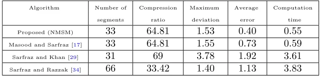
The results obtained for the “Kanji” character are presented in Figure5 and tabulated in Table2. The image of “Kanji” character and its boundary are shown in Figures 5(a) and 5(b), respectively. Figure 5(c) shows the boundary along with the corner points which are marked with a square (■). The results of the presented method for this shape are given in Figure5(d). The outline captured with algorithm [17] is shown in Figure5(e). The result obtained by Sarfraz and Khan [29] can be seen in Figure 5(f). The outline generated by means of method [34] is given in Figure5(g). It should be noted that the results of Tables1and2 are achieved by different systems.
Galley
Pro
of
Table 1: Quantitative comparison for the Arabic word “Sabr”.Algorithm Number of Compression Maximum Average Computation
segments ratio deviation error time
Proposed (NMSM) 28 46.43 1.92 0.44 0.79
Masood and Sarfraz [17] 27 48.15 2.21 1.38 0.83
Sarfraz and Razzak [34] atτ= 3 66 19.70 1.71 1.07 3.79 Sarfraz and Razzak [34] atτ= 2 98 13.27 1.39 0.91 2.58
Table 2: Quantitative comparison for the “Kanji” character.
Algorithm Number of Compression Maximum Average Computation
segments ratio deviation error time
Proposed (NMSM) 33 64.81 1.53 0.40 0.55
Masood and Sarfraz [17] 33 64.81 1.55 0.73 0.59
Sarfraz and Khan [29] 31 69 3.78 1.92 3.61
Sarfraz and Razzak [34] 66 33.42 1.40 1.13 3.83
• The method proposed in this study protects an appropriate equilibrium among the compression ratio and the fitting error.
• The proposed method avoids time consuming procedures, such as least square fitting, and uses one of the popular derivative-free free operations (i.e., the NelderMead simplex method ) that is simple and fast.
• The average error, maximum deviation, and the computation time are lesser than the results obtained by other methods in the current liter-ature [17,29,34].
• The number of segments generated by method [34] is very high because the corner detection and the subdivision algorithms are suboptimal. The suboptimal corner points are indicated by arrows in Figures4(f), 4(g), and5(g). This method also suffers from a long computation time. This is due to the use of least squares fitting and control parameters.
• Computation of the outline by means of method [29] takes too long and has errors. The least squares curve fitting and the noise filtering procedure are the main causes for these disadvantages. It is shown with an arrow in Figure5(f).
Galley
Pro
of
(a) Original image. (b) Boundary of original image.
(c) Boundary with cor-ner points.
(d) Proposed method (NMSM). (e) Masood and Sarfraz [17].
(f) Sarfraz and Razzak [34] atτ= 3. (g) Sarfraz and Razzak [34] atτ= 2.
Galley
Pro
of
(a) Original image. (b) Outline of original image.
(c) Boundary with cor-ner points.
(d) Proposed method (NMSM). (e) Masood and Sarfraz [17].
(f) Sarfraz and Khan [29]. (g) Sarfraz and Razzak [34].
Figure 5: Captured shape of the Kanji character with different methods.
6 Conclusion
Galley
Pro
of
the cubic B´ezier curve. It increases the speed of convergence and the quality of curve fitting. As a result, the introduced approximation scheme is much faster than traditional approaches and helps to capture a better fit with a desirable precision. Through a comparison of our method with previous ap-proaches and considering the simulation results, it emerges that the method has such advantages as appropriate equivalency between the compression ra-tio and the fitting error, low deviara-tion error, and low computara-tion time.References
1. B´ezier, P.Numerical control; mathematics and applications, John Wiley & Sons, 1972.
2. Biswas, S. and Lovell, B.C.B´ezier and splines in image processing and machine vision, Springer Science & Business Media, 2007.
3. Cabrelli, C.A. and Molter, U.M. Automatic representation of binary images,IEEE Trans. Pattern. Anal. Mach. Intell., 12 (1990), 1190–1196.
4. Chetverikov, D. and Szabo, Z.A simple and efficient algorithm for de-tection of high curvature points in planar curves,proc. of 23rd workshop of Australian Pattern Recognition Group, Steyr, (1999), 175–184.
5. Conn, A.R., Scheinberg, K. and Vicente, L.N.Introduction to derivative-free optimization, MOS-SIAM Series on Optimization, 2009.
6. Farin, G. Curves and surfaces for computer-aided geometric design: a practical guide, Academic Press, 1997.
7. Freeman, H. On the encoding of arbitrary geometric configurations,
IEEE Trans. Comput., 2 (1961), 260–268.
8. Hassanien, A.E., Grosan, C. and Tolba, M.F.Applications of intelligent optimization in biology and medicine: Current trends and open prob-lems, Springer, 2015.
9. Hussain, M., Hussain, M.Z., and Sarfraz, M. Shape-preserving polyno-mial interpolation scheme,Iran. J. Sci. Technol. Trans. A Sci., 40 (2016), no. 1, 9–18.
10. Hussain, M.Z., Hussain, F. and Sarfraz, M. Shape-preserving positive trigonometric spline curves, Iran. J. Sci. Technol. Trans. A Sci. 42 (2018), no. 2, 1–13.
11. Itoh, K. and Ohno, Y.A curve fitting algorithm for character fonts,
Galley
Pro
of
12. Khan, M.S., Ayob, A. F.M., Isaacs, A. and Ray, T.A novel evolution-ary approach for 2d shape matching based on B-spline modeling, Proc. Congr. Evol. Comput., (2011), 655–661.13. Klein, K. and Neira, J.Nelder–Mead simplex optimization routine for large-scale problems: A distributed memory implementation, Comput. Econ., 4 (2014), 447–461.
14. Lagarias, J.C., Reeds, J.A., Wright, M.H. and Wright, P.E.Convergence properties of the nelder–mead simplex method in low dimensions,SIAM. J. Optim. , 9 (1998), no. 1, 112–147.
15. Marji, M. and Siy, P.A new algorithm for dominant points detection and polygonization of digital curves, Pattern. Recognit., 10 (2003), 2239– 2251.
16. Masood, A. and Haq, S.A.Object coding for real time image processing applications, Pattern Recognition and Image Analysis. ICAPR 2005. Lecture Notes in Computer Science, vol 3687. Springer, Berlin, Heidel-berg.
17. Masood, A. and Sarfraz, M. An efficient technique for capturing 2d objects,Comput. Graph., 32 (2008), no 1, 93–104.
18. Masood, A. and Sarfraz, M.Capturing outlines of 2d objects with b´ezier cubic approximation,Image Vis. Comput., 6 (2009), 704–712.
19. Nelder, J. A., and Mead, R.A simplex method for function minimiza-tion,Comput. J., 7 (1965), no. 4, 308–313.
20. Piegl, L. and Tiller, W.The NURBS book. Springer Science & Business Media, 2012.
21. Plass, M. and Stone, M.Curve-fitting with piecewise parametric cubics, Comput. Graph., 17 (1983), no 3, 229–239.
22. Powell, S. Applications and enhancements of aircraft design optimiza-tion techniques, PhD thesis, University of Southampton, 2012.
23. Salomon, D.Curves and surfaces for computer graphics, Springer Sci-ence & Business Media, 2007.
24. Sarfraz, M. Some algorithms for curve design and automatic outline capturing of images, Int. J. Image. Graph., 2 (2004), 301–324.
25. Sarfraz, M. Computer-aided intelligent recognition techniques and ap-plications, Wiley Online Library, 2005.
Galley
Pro
of
27. Sarfraz, M. Capturing image outlines using simulated annealing ap-proach with conic splines, The Proceedings of the International Con-ference on Information and Intelligent Computing, (2011), 152–157.28. Sarfraz, M. and Khan, M. Automatic outline capture of arabic fonts,
Inf. Sci., 3 (2002), 269–281.
29. Sarfraz, M. and Khan, M. An automatic algorithm for approximating boundary of bitmap characters,Future. Gener. Comput. Syst., 8 (2004), 1327–1336.
30. Sarfraz, M. and Masood, A.Capturing outlines of planar images using b´ezier cubics,Comput. Graph., 5 (2007), 719–729.
31. Sarfraz, M., Masood, A. and Asim, M.R. A new approach to corner detection,Computer Vision and Graphics 32 (2006), 528533
32. Sarfraz, M. and Raza, A.Visualization of data with spline fitting: a tool with a genetic approach,CISST, 97(2002), 99–105.
33. Sarfraz, M. and Raza, S.A. Capturing outline of fonts using genetic algorithm and splines, Proceedings of IEEE International Conference on Information Visualization-IV’2001-UK, USA:IEEE Computer Soci-ety Press, (2001), 738–743.
34. Sarfraz, M. and Razzak, M. An algorithm for automatic capturing of the font outlines,Comput. Graph., 5 (2002), 795–804.
35. Sarfraz, M., Riyazuddin, M. and Baig, M.Capturing planar shapes by approximating their outlines, J. Comput. Appl. Math., 1 (2006), 494– 512.
36. Sohel, F.A., Karmakar, G.C., Dooley, L.S. and Arkinstall, J.Enhanced bezier curve models incorporating local information, Proc. IEEE. Int. Conf. Acoust. Speech. Signal. Process., 4 (2005), 253–256.
37. Tang, Y. Y., Yang, F., and Liu, J.Basic processes of chinese character based on cubic b-spline wavelet transform,IEEE. Trans. Pattern. Anal. Mach. Intell., 12 (2001), 1443–1448.
38. Zheng, W., Bo, P., Liu, Y., and Wang, W. Fast B-spline curve fitting by L-BFGS,Comput. Aided. Geom. Des., 7 (2012), 448–462.