in the population sciences published by the Max Planck Institute for Demographic Research Doberaner Strasse 114 · D-18057 Rostock · GERMANY www.demographic-research.org
DEMOGRAPHIC RESEARCH
VOLUME 4, ARTICLE 7, PAGES 185-202
PUBLISHED 17 MAY 2001
www.demographic-research.org/Volumes/Vol4/7/
DOI: 10.4054/DemRes.2001.4.7
Manhood trials and the law of mortality
Harald Hannerz
1. Introduction 186
2. Some gender comparisons 189
3. Traffic casualties 190
4. A mathematical treatment of the accident hump 191
Manhood trials and the law of mortality
Harald Hannerz 1
Abstract
The present paper introduces a continuous eight-parameter survival function intended to model mortality in modern male populations.
1. Introduction
“Mathematically a statistical model is essentially a specified family of admissible probability distributions. [...] A statistical model should give a correct and as far as possible an explanatory description of the actual data structure. It must also be statistically analysable, in practice as well as in theory. [...] Faced with the complex physical reality, with imprecise knowledge as to causes and mechanisms behind the variation in data, and equipped with limited mathematical and numerical resources, one often has to settle with a model that describes data in rough outlines. [...] A good model can thereby be compared with a good caricature: A strongly simplified picture, that bears in mind and often exaggerates some distinctive features, but still clearly resembles reality.” (Sundberg, 1981. See Note 1)
In accordance with the above definition of a statistical model, several mathematical expressions to describe human mortality at all ages simultaneously have been devised. With degrees of simplification as criteria these models can roughly be divided into two types. The first type states that mortality is decreasing rapidly with age during infancy, thereafter it levels out and starts to increase slowly until the age of senescence where the increase becomes more and more rapid with age. The second type is more complex in that it, apart from the above features, also allows for an added mortality risk associated with the passage into adulthood. The laws of Wittstein (1883), Petrioli (1981) and Siler (1983) are examples of the first type, while the laws of Thiele (1872) and Heligman & Pollard (1980) are examples of the second type. An increased mortality among people in early adulthood is often referred to as an accident hump (Heligman and Pollard, 1980; Hartmann, 1987; Kostaki, 1992) believed to be caused mainly by accidents among males and accidents and maternal mortality among women (Heligman and Pollard, 1980).
In a recent thesis (Hannerz 1999), the following formula, which belongs to the first type of models, was proposed:
where F(x) denotes the probability that a new-born person will be dead within x years, G(x) is the corresponding logodds, log(F/(1-F)), and c and the ai’s are parameters. The
parameter a0 may be negative but the rest of the parameters should be positive.
By transforming equation (1) we also obtain analytical expressions for the survival function
[
( )]
11
)
(
1
)
(
x
=
−
F
x
=
+
e
G x −l
(2)the probability density function
[
( )]
2 ) (1
)
(
x G x Ge
e
dx
dG
dx
dF
x
f
+
=
=
(3)and the hazard function (the force of mortality)
) ( ) (
1
)
(
1
)
(
)
(
Gxx G
e
e
dx
dG
x
F
x
f
x
+
=
−
=
µ
.
(4)Graphic representations of equation (1)-(4) are given in figure 1, where the formula has been fitted to mortality among Swedish females in 1986.
Figure 1: The functions f, µ, l and G, fitted to mortality in the female population of Sweden 1986. The grey bars in the top left picture constitute the un-graduated frequency function.
Reports about gang wars in the big cities of USA, where young men kill each other, and in Sweden where different motorcycle bands meet in mortal combat, as well as debates on the maturity of young males in regard to driver licences etc., seem to indicate a generally raised mortality risk for young men.
In a book edited by Cohen (1991) the topic of rites of passage into manhood, is discussed. One of many global examples is teenage ”surfistas” riding atop speeding trains swerving through the hills above Rio de Janeiro: ”If they touch the electric lines or fail to duck at the right moment, they risk serious injury or death.” This particular discussion ends with the following quotation: ”As mythologist Joseph Campbell
0.0 0.2 0.4 0.6 0.8 1.0
0 20 40 60 80 100
Age
l
-6 -4 -2 0 2 4 6
0 20 40 60 80 100
Age
G
0.0001 0.001 0.01 0.1 1
0 20 40 60 80 100
Age
pointed out, boys everywhere have a need for rituals marking their passage to manhood. If society does not provide them they will inevitably invent their own.” (Cohen 1991).
The first aim of the present work was to find out if, among Swedish males, there is still a statistically important added risk associated with the passage into manhood. If this is the case then a second aim would be to find out if the term accident hump gives an appropriate description of such a risk elevation, and a third aim would be to develop a continuous and analytically expressible survival function that describes mortality reasonably well among men.
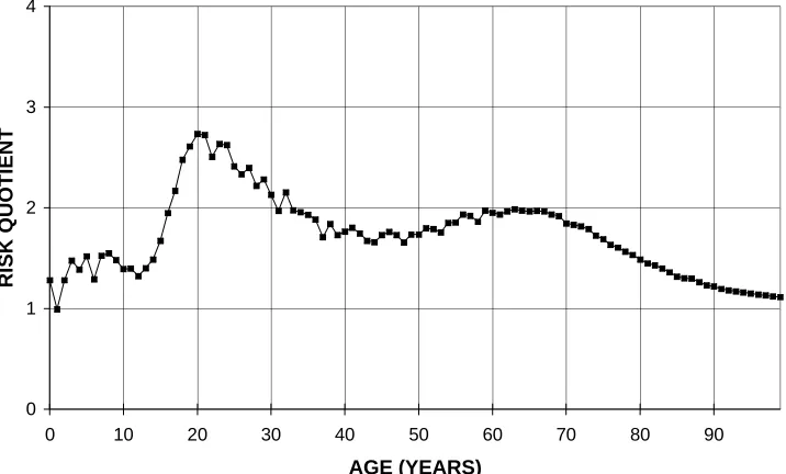
2. Some gender comparisons
Figure 2: The average empirical mortality risk for Swedish males divided by that for Swedish females 1968-1992, plotted against age.
3. Traffic casualties
A possible explanation of the bulge in the risk-ratio between men and women during the passage into adulthood is that reckless driving could be regarded as a manhood trial so that the traffic casualties would cause a non-negligible bulge in the density function of the men but not in that of the women. The deaths in 1982 caused by traffic were therefore removed from the data and new goodness-of-fit tests, of the model described by equation (1), were performed. Now, without the traffic casualties, the chi-square sum was 138 for males and 140 for females. From this test we may conclude that the only reason why equation (1) does not fit a Swedish male mortality experience would be an accident hump in the beginning of adulthood.
0 1 2 3 4
0 10 20 30 40 50 60 70 80 90
AGE (YEARS)
Figure 3: The proportion of deaths among Swedish males 1982, caused by traffic accidents.
4. A mathematical treatment of the accident hump
Pearson (1895) suggested that all different causes of death could be divided into five types of mortality. Each type would follow its own frequency function, and by conditioning on type of mortality a frequency function for the total mortality would be obtained by a weighted sum of the five conditional functions. He also proposed specific families of frequency functions for each of the five types of mortality, and subsequently wound up with a model for all-cause mortality that involved 14 parameters to be determined from the sample. Although the mortality model of Pearson might be considered too complex to be useful in actuarial and demographic work (Brass, 1974), the approach to the problem — the application of a mixture distribution to handle multimodality—has been broadly embraced by statisticians (e.g. Moore and Gray 1993; McLaren et al. 1991; Boos and Brownie 1991; Mendell, Thode and Finch 1991; Hall and Titterington 1984; Larson 1985; Basford and McLachlan 1985; Davenport, Bezdek
0% 10% 20% 30% 40%
0-4 5-9
10-14 15-19 20-24 25-29 30-34 35-39 40-44 45-49 50-54 55-59 60-64 65-69 70-74 75-79 80-84 85-89 90+
AGE (YEARS)
If we assume that there is such a thing as a manhood trial —an added hazard intentionally or unintentionally imposed on males, either by themselves or by the environment, which is associated mainly with the passage into manhood— and that some males would die as a direct consequence of such a trial, then mortality among males could be divided into two types: mortality from manhood trials and mortality from other causes. A function that fits a male mortality experience would thus be obtained by the following scheme: Let F1(x) be the death distribution given that the subject will die a ”natural” death and F2(x) be the distribution given that the death is caused by a ”manhood trial”. Let α be the probability that a death will be natural; then F(x) = αF1(x) + (1-α)F2(x).
The following model was tried on the Swedish males of 1982:
(
)
(
)
+
+
−
=
+
+
−
=
+
−
+
+
=
−
+
=
c
e
a
x
a
x
a
a
x
G
c
e
a
x
a
x
a
a
x
G
e
e
e
e
x
F
x
F
x
F
cx cx x G x G x G x G 3 2 2 5 4 2 3 2 2 1 0 1 ) ( ) ( ) ( ) ( 2 12
)
(
2
)
(
1
1
1
)
(
1
)
(
)
(
2 2 1 1α
α
α
α
(5)Table 1: Parameter estimates for Equation (2) fitted to mortality in the Swedish male population 1982.
a0 a1 a2 a3 a4 a5 c α
-4.627 0.208 1.541*10-3 4.715*10-7 6.034 154.9 0.1379 0.9945
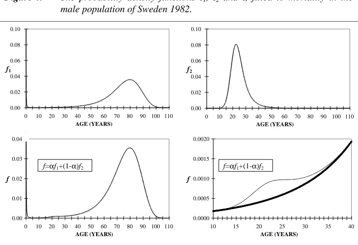
Figure 4: The probability density functions f1, f2 and f, fitted to mortality in the male population of Sweden 1982.
As seen in equation (5), G2(x) contains 5 parameters, but (for the sake of parsimony) only two of those, a4 and a5, are unique to that function while the other three are shared with G1(x). The reader might wonder if those two parameters are sufficient to render f2 plastic enough to attain the different shapes that one might associate with a death distribution for people who die from “manhood trials”. Experiments have shown that they are. The effect on f2 when a4 is varied, while the other parameters retain the values
0.00 0.02 0.04 0.06 0.08 0.10
0 10 20 30 40 50 60 70 80 90 100 110
AGE (YEARS)
f1
0.00 0.02 0.04 0.06 0.08 0.10
0 10 20 30 40 50 60 70 80 90 100 110
AGE (YEARS)
f2
0.00 0.01 0.02 0.03 0.04
0 10 20 30 40 50 60 70 80 90 100 110
AGE (YEARS)
f
f=αf1+(1-α)f2
0.0000 0.0005 0.0010 0.0015 0.0020
10 15 20 25 30 35 40
AGE (YEARS)
f
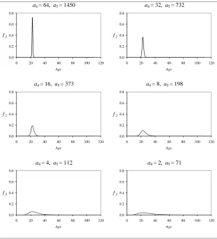
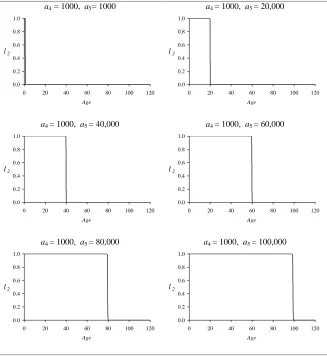
of f2 at the same place, is shown in figure 7. The ultimate test would of course be if a completely rectangular survival function could be obtained, i.e. if we could describe the mortality distribution even if all manhood trials were to occur only at one specific age. In figure 8 it is shown that such distributions can be obtained without having to vary any other parameters but a4 and a5.
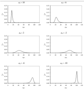
Figure 5: The effect on f2 when a4 is varied, while the other parameters retain the values given in table 1.
a4 = 10 a4 = 6
a4 = 2 a4 = -2
a4 = -6 a4 = -10
0.00 0.05 0.10 0.15 0.20 0.25
0 20 40 60 80 100 120
Age f2
0.00 0.05 0.10 0.15 0.20 0.25
0 20 40 60 80 100 120
Age f2
0.00 0.05 0.10 0.15 0.20 0.25
0 20 40 60 80 100 120
Age f2
0.00 0.05 0.10 0.15 0.20 0.25
0 20 40 60 80 100 120
Age f2
0.00 0.05 0.10 0.15 0.20 0.25
0 20 40 60 80 100 120
Age f2
0.00 0.05 0.10 0.15 0.20 0.25
0 20 40 60 80 100 120
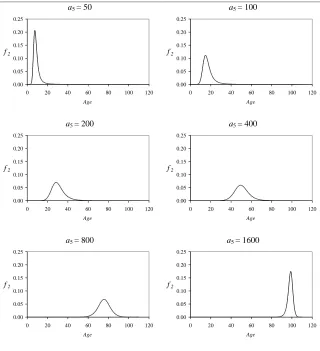
Figure 6: The effect on f2 when a5 is varied, while the other parameters retain the values given in table 1.
a5 = 50 a5 = 100
a5 = 200 a5 = 400
a5 = 800 a5 = 1600
0.00 0.05 0.10 0.15 0.20 0.25
0 20 40 60 80 100 120
Age
f2
0.00 0.05 0.10 0.15 0.20 0.25
0 20 40 60 80 100 120
Age
f2
0.00 0.05 0.10 0.15 0.20 0.25
0 20 40 60 80 100 120
Age
f2
0.00 0.05 0.10 0.15 0.20 0.25
0 20 40 60 80 100 120
Age
f2
0.00 0.05 0.10 0.15 0.20 0.25
0 20 40 60 80 100 120
Age
f2
0.00 0.05 0.10 0.15 0.20 0.25
0 20 40 60 80 100 120
Age
Figure 7: The effect on f2 when a4 and a5 are varied, while the other parameters retain the values given in table 1.
a4 = 64, a5 = 1450 a4 = 32, a5 = 732
a4 = 16, a5 = 373 a4 = 8, a5 = 198
a4 = 4, a5 = 112 a4 = 2, a5 = 71 0.0
0.2 0.4 0.6 0.8
0 20 40 60 80 100 120
Age
f2
0.0 0.2 0.4 0.6 0.8
0 20 40 60 80 100 120
Age
f2
0.0 0.2 0.4 0.6 0.8
0 20 40 60 80 100 120
Age
f2
0.0 0.2 0.4 0.6 0.8
0 20 40 60 80 100 120
Age
f2
0.0 0.2 0.4 0.6 0.8
0 20 40 60 80 100 120
Age
f2
0.0 0.2 0.4 0.6 0.8
0 20 40 60 80 100 120
Age
Figure 8: The effect on the survival function, l2, when a4 and a5 are varied, while the other parameters retain the values given in table 1.
a4 = 1000, a5= 1000 a4 = 1000, a5 = 20,000
a4 = 1000, a5 = 40,000 a4 = 1000, a5 = 60,000
a4 = 1000, a5 = 80,000 a4 = 1000, a5 = 100,000 0.0
0.2 0.4 0.6 0.8 1.0
0 20 40 60 80 100 120
Age
l2
0.0 0.2 0.4 0.6 0.8 1.0
0 20 40 60 80 100 120
Age
l2
0.0 0.2 0.4 0.6 0.8 1.0
0 20 40 60 80 100 120
Age
l2
0.0 0.2 0.4 0.6 0.8 1.0
0 20 40 60 80 100 120
Age
l2
0.0 0.2 0.4 0.6 0.8 1.0
0 20 40 60 80 100 120
Age
l2
0.0 0.2 0.4 0.6 0.8 1.0
0 20 40 60 80 100 120
Age
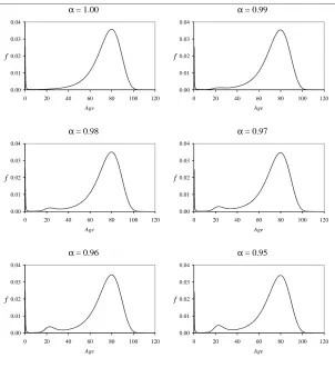
Figure 9: The effect on f2 when α is varied, while the other parameters retain the values given in table 1
α= 1.00 α= 0.99
α= 0.98 α= 0.97
α= 0.96 α= 0.95
0.00 0.01 0.02 0.03 0.04
0 20 40 60 80 100 120
Age f
0.00 0.01 0.02 0.03 0.04
0 20 40 60 80 100 120
Age f
0.00 0.01 0.02 0.03 0.04
0 20 40 60 80 100 120
Age f
0.00 0.01 0.02 0.03 0.04
0 20 40 60 80 100 120
Age f
0.00 0.01 0.02 0.03 0.04
0 20 40 60 80 100 120
Age f
0.00 0.01 0.02 0.03 0.04
0 20 40 60 80 100 120
To summarise, many different shapes and locations of the accident hump can be obtained by varying the parameters a4 and a5. The only reason for not dropping the parameters a2, a3 and c in G2 is to make sure that the mean expectation of life, for the people dying from “manhood trials”,
[ ]
=
∫
∞ 02
(
x
)
dx
xf
X
E
(6)exists and is finite. According to a theorem (Hannerz 2001) the above expectation will always exist and will be finite if at least one of the last two terms in G2 is kept in the model.
5. Discussion
Notes
1. The original wording is in Swedish. This is a free translation.
References
Åstrand PO, Rodahl K. (1986). Textbook of work physiology. Physiological bases of exercise. Third edition. New York: McGraw-Hill Inc. p. 343.
Basford KE, McLachlan GJ. (1985). “Likelihood estimation with normal mixture models.“ Applied Statistics, 34:282-289.
Bickel PJ, Doksum KA. (1977). Mathematical statistics — basic ideas and selected topics. New Jersey: Prentice Hall.
Boos DD, Brownie C. (1991). “Mixture models for continuous data in dose-response studies when some animals are unaffected by treatment.” Biometrics, 47:1489-1504.
Brass W. (1974). “Mortality models and their use in demography.” Transactions of the Faculty of Actuaries, 33:122-133.
Cohen D [Editor]. (1991). The circle of life — rituals from the human family album. London: The Aquarian Press.
Davenport JW, Bezdek JC, Hathaway RJ. (1988). “Parameter estimation for finite mixture distributions.” Comput Math Applic, 15:819-828.
Hall P, Titterington DM. (1984). “Efficient nonparametric estimation of mixture proportions.“ Journal of the Royal Statistical Society, 46:465-473.
Hannerz H. (1999). Methodology and applications of a new law of mortality. Lund: Department of Statistics. University of Lund, Sweden.
Hannerz H. (2001). “Presentation and derivation of a five-parameter survival function
intended to model mortality in modern female populations.” Scandinavian
Actuarial Journal, (In Press).
Heligman M, Pollard JH. (1980). “The age pattern of mortality.” Journal of the Institute of Actuaries, 107:49-80.
Kostaki A. (1992). Methodology and applications of the Heligman-Pollard formula. Lund: Department of Statistics. University of Lund, Sweden.
Larson MG. (1985). “A mixture model for the regression analysis of competing risks data.” Applied statistics, 34:201-211.
McLaren CE, Wagstaff M, Brittenham GM, Jacobs A. (1991). “Detection of two-component mixtures of lognormal distributions in grouped doubly truncated data — analysis of red blood cell volume distributions.” Biometrics, 47:607-622.
Mendell NR, Thode HC, Finch SJ. (1991). “The likelihood ratio test for the two-component normal mixture problem — power and sample size analysis.” Biometrics, 47:1143-1148.
More DH, Gray JW. (1993). “Derivative domain fitting — a new method for resolving a mixture of normal distributions in the presence of a contaminating background.” Cytometry, 14:510-518.
Mortensen EL. (1997). “Aldring og intelligens.” Gerontologi og samfund, 13:76-78.
Pearson K. (1895). “Contributions to the mathematical theory of evolution. II. Skew variation in homogenous material.” Philosophical Transactions of the Royal Society of London, 186:343-414.
Pearson K. (1900). “On the Criterion that a given System of Deviations from the Probable in the case of a Correlated System of Variables is such that it can be
reasonably supposed to have arisen from Random Sampling.” The London,
Edinburgh and Dublin Philosophical Magazine and Journal of Science, 50:157-175.
Petrioli L. (1981). A new set of models of mortality. Paper presented at IUSSP seminar on methodology and data collection, Dakar, Senegal, reprinted by Universita degli Studi di Siena, Italy.
Siler W. (1983). “Parameters of mortality in human populations with widely varying life spans.” Statistics in Medicine, 2:373-380.
Sinclair D. (1985.) Human growth after birth. Fourth edition. Oxford: Oxford University Press. p. 229.
Thiele TN. (1872). “On a mathematical formula to express the rate of mortality throughout life.” Journal of the Institute of Actuaries, 16:313-329.