Studies on the effects of parameters on the convergence of local radial point interpolation method (LRPIM)

________________

*_{Corresponding author}

Received March 2, 2016

922

Available online at http://scik.org

J. Math. Comput. Sci. 6 (2016), No. 5, 922-933

ISSN: 1927-5307

STUDIES ON THE EFFECTS OF PARAMETERS ON THE CONVERGENCE OF

LOCAL RADIAL POINT INTERPOLATION METHOD (LRPIM) AHMED MOUSSAOUI* _{AND TOURIA BOUZIANE}

Department of physics, Faculty of Sciences, Moulay Ismail University, B.P.11201 Meknes, Morocco

Copyright © 2016 Ahmed Moussaoui and Touria Bouziane. This is an open access article distributed under the Creative Commons Attribution License, which permits unrestricted use, distribution, and reproduction in any medium, provided the original work is properly cited.

Abstract: Numerical solutions in physical engineering problems need appropriate numerical approximation methods. Meshless methods have attracted increasing attention in recent years for seeking of approximate solutions of initial boundary value problem governed by partial differential equations. In this paper, we will present a study of a 2D problem of an elastic homogenous rectangular plate by using the local radial point interpolation method (LRPIM). We investigate the convergence and accuracy of method LRPIM and numerical values are presented to specifying the convergence domain by precising maximum and minimum values as a function of distribution nodes number and by using the radial basis function: Gaussian (EXP). It also presents a comparison with numerical results for different materials and the radial basis functions (RBF). Finally, a comparative study of numerical results with analytical solutions is presented.

Keywords: Linear Elasticity; Rectangular Plate; Meshless Method LRPIM; Support Domain; Radial Basis Function.

2010 AMS Subject Classification: 65L60.

1 Introduction

data.

So a class of meshfree methods has developed and become a very attractive alternative for computer modelling and simulation of problems in engineering and science. These methods such as meshless [4-8] do not require a mesh to discretize the problem domain (in a specific area) and the approximation functions are constructed using only with a set of scattered nodes, and no element or connectivity between nodes is needed.

Recently Meshless method has attracted more attention from researchers and it is regarded as a potential numerical method in computational mechanics. Several meshless methods, such as smooth particle hydrodynamics (SPH) method [4-6], element free Galerkin (EFG) method [7], meshless local Petrov-Galerkin (MLPG) method [8-9], the point interpolation methods (PIM)[10-11] and local radial point interpolation method (LRPIM) proposed by Liu et al. [11]. In LRPIM, the point interpolation developed by the radial function basis is used to construct shape functions with delta function property. The widely used radial basis functions (RBFs) are multi-quadric (MQ), Gaussian (EXP) [12] and thin plate spline (TPS) function [13]. In this paper, the local weak forms are developed using weighted residual method locally from the partial differential equation of elastostatic linear 2D solids. We discus the effects of some parameters for radial basis function, and also the effects of size parameter of support and quadrature domains on the performance of the local radial point interpolation method LRPIM. Numerical results are presented to describe the convergence and accuracy, validity and efficiency of the present methods.

The aims of this paper are to study the effect on convergence and accuracy of LRPIM methods of different size parameters by varying



s (the size of the support domain) and

2

Q 



(quadrature domain) was fixed. In LRPIM methods, the support domain is equal to

influence domain. For fixed values of



_s and



_Q 2, the effect of nodes distributions field

2.Radial point interpolation shape functions

) x (

uh is composed of two part:Pj(x)Polynomial basis functions and Ri(x)the radial basis

functions RBFs [10-11]:





    n 1 i m 1 j j j i i h b (x) P a (x) R (x)

u (1)

n is the number of field nodes in the local support domain and m is the number of polynomial terms.

Radial basis is a function of distance r: i 2

2

i) (y y )

x (x

r     (2) The above equation (1) can be expressed in the matrix form [10]

b P a R

U₁     (3) Where U₁The vector of function values:U₁ 



u₁, u₂, u₃,..., u_n



T

R The moment matrix of RBFs, P the moment matrix of Polynomial basis function and a, b the values of unknowns coefficients (Radial and Polynomial)

We note that, to obtain the unique solutions of Eq. (2), the constraint conditions should be

applied as follows [14]:



   n 1 i i

ij(x)a 0 j 1, 2, ...,m

P (4)

By combining Eqs. (3) and (4) yields a set of equations in the matrix form:

_T Ga₀ b a P P R U

U _

                   0 0 1

1 (5)

The unknowns vector can be obtained by inversion of the matrix _

      0 T P P R G

Substitution of the vector obtained by inversion of matrixGinto Eq. (1) leads to:



   n 1 i i i h u (x)

u 1 

T

U (x)

Φ (6)

3. Local weak form method LRPIM



_ij,j

(

x

)



b

_i

(

x

)



0

(7)



ij

n

j



t

0i on t (8)

u

_i



u

0_i on



_u (9)

Where in : [ xx, yy, xy]

T    

σ is the stress vector, [bx,by]

T 

b the body force vector.

) n , n ( 1 2 

n denotes the vector of unit outward normal at a point on the natural boundaries

0

t is the prescribed effort, [u₁,u₂]the displacement components in the plan and [u₁0,u0₂] on the essential boundaries.

In the local Petrov-Galerkin approaches [7], one may write a weak form over Q a local

quadrature domain (for node I), which may have an arbitrary shape, and contain the point xQ in

question, see Fig. 1. The generalized local weak form of the differential Eq. (7) is obtained by:

( (x) b (x)) d 0 Q

I i j

,

ij  











(10) Where _Q is the local domain of quadrature for node I and _I is the weight or test function,

) ( CK

I 

  [8].

Figure 1. The local sub-domains around point x_Q and boundaries Using the divergence theorem [8] in Eq. (10), we obtain:

n d d b d 0

Q Q

Q ij j I ij I,j i I

 



_

_



           (11)

Where Q QiQu Qt

Qi

 : The internal boundary of the quadrature domain

Qt

 : The part of the natural boundary that intersects with the quadrature domain

Qu

 : The part of the essential boundary that intersects with the quadrature domain

We can then change the expression of équ(11):

0 d b d d n d n d n Q Q

Qi ij j I Qu ij j I Qt ij j I ij I,j i I

 

 



_

_



   



   



           (12)

Using the RPIM shape functions (see sub-section 2), we can approximate the trial function for the displacement at a point x (xS ) as eq.(6)

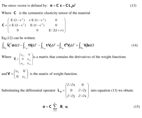
The stress vector is defined by: σC εCLduh (13)

Where C is the symmetric elasticity tensor of the material

                ) 1 ( 2 / E 0 0 0 ) 1 /( E ) 1 /( E 0 ) 1 /( E ) 1 /( E 2 2 2 2        C

Eq.(12) can be written:











    Q Qi Qu Qi Q d d d d d T    

 V σ  tV  tV  t VI  VIb 

0 I

I

I (14)

Where            x , I y , I y , I x , I I 0 0    

V is a matrix that contains the derivatives of the weight functions

and _       I I 0 0  

V is the matrix of weight function.

Substituting the differential operator

                   x / y / y / 0 0 x / d

L into equation (13) we obtain:





 nt

1 I I I u B C

Where            x , I y , I y , I x , I 0 0     I

B . By using the matrix

           1 2 2 1 n n n 0 0 n n

L , the tractions of a point x can be

written as: tLT_nσ (16) Substituting Eqs. (15, 16) into Eq. (14), we obtain the discrete systems of linear equations for the node I.





















 Qt Q

t Qu Qi Q d d t ] d d d

[ _{I I}

n 1 I I I T

I _{   }

 V CB  L CB V  L CB V  u V  Vb 

0 I T n I T n

I I (17)

The matrix form of Eq. (17) can be written as in matrix form:



  t n 1 I I I

Iu f

K (18)

Where expression of nodal matrix K_Iis













Qu Qi Q d d

d _{I I}

T

I _{ }

 V CB  L CB V  L CB V 

K T _I

n I

T n I

I (19)

And nodal force vector with contributions from body forces applied in the problem domains:









Qt Q

d d

t _{I I}

 V   V b 

f 0

I (20)

Wheren0 denote the set of the nodes in the support domain S of pointxQ.

Two independent linear equations can be obtained for each node in the entire problem domain and by assembling all these 2*n equations to obtain the final global system equations:

k

2n*2n

u

2n *1



f

2n*1 (21)

To solve the precedent system, the standard Gauss quadrature formula is applied with 16 Gauss points [7, 15] for calculating integrals in Eqs (19, 20) on both boundary and domain.

The size of quadrature domain is specified by setting _Q 2 and a regular distribution of nodes on the mid-surface of plate in (x, y) plane is employed.

4. Numerical 2D elastostatic example

34 . 0



 _; 6 2

m / N 10 . 17

E _, 0.33 _{) respectively} Dimension of the plate are denoted: height}

m 12

D , length L48m, the thickness: unit and finally for Loading: P103N 

Figure 2. Cantilever plate subjected to distributed traction at the free end.

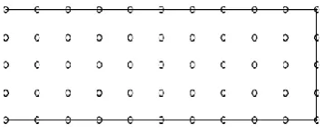
Figure 3. Regular field nodes distribution on the problem domain and boundaries

In our numerical calculations, were considered many regular distributions of nodes nt: 18,

55, 91, 175 and 189. To calculate the error energy, a background cells are required; then, for

each value of n_t the number of cell was varied. To obtain numerical values, the distribution of

the deflection through the plates, size of support domain is varied and _Q 2 size of the

quadrature domain.

The sizes of support domain _s(quadrature domain_Qresp.) are defined by: d_s _sd_c

(r_Q _Qd_cIresp.) whered_c( d_cI resp) is the nodal spacing near node I (Fig. 3) and _s(_Q

resp) is the size of the support domain_s( local quadrature domains resp) for node I. The sizes

of support domain _s( quadrature domains resp) will be respectively determined in x and y

directions. For simplicity Sx Sy S(Qx Qy Qresp) is used for s(Q resp).

5. Results and Discussions

the test functions in the LRPIM local weak-form.

Throughout this section and for all calculations, Qwas fixed and the value 2 (Q 2).

5.1Results numerical of the radial basis functions RFB-EXP

We studied the effect of the parameter the radial basis functions RBF-EXP on convergence of the LRPIM method.

1,5 2,0 2,5 3,0 3,5 4,0 4,5 5,0 5,5 0,0

0,2 0,4 0,6 0,8 1,0

En

e

rg

y

e

rr

o

r

Steel Copper, 55 nodes Steel Copper, 91 nodes Steel Copper, 175 nodes

_S

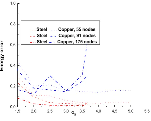
Figure 4 Variation of the energy error as a function of _Sfor two materials and different values of n_t

Figure 4 shows the variation of the error energy as a function of _S for two studied materials: steel and copper (different values of E and  ) and for different values of the number of nodesn_t 55, 91, 175 of the radial basis function RBF-EXP.

We found that all of the curves of the two materials have identical shapes to a fixed value of _S,

the curves of steel are more stable for all values of n_t, the steel has a good convergence.

For copper, the method converges for nt= 55 and 91, but nt= 175 from S= 3.5, the method

is divergent.

We used only two materials for LRPIM method with the radial basis function RBF-EXP. The ends of the domain of convergence are similar as those found by the MLPG method [17]

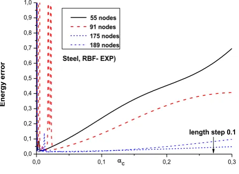
In figure 5-6 shows the variation of the error energy as a function of C of the radial basis

LRPIM method is not convergent, but only that of steel, the method has a good convergence, the

domain of convergence of the steel is wide (0.001C 0.3) with respect to other materials.

But for the other materials, the domain of convergent is 0.006C 0.3.

Finally, we can also say that the domain of the convergence is broader than that given in the

references [11, 18] which gave the interval 0.003_C 0.03for a single material. The method is convergent when the number n_t is very large on a larger domain (for steel Figure 6).

0,000 0,005 0,010 0,015 0,020 0,025 0,030 0,1

0,2 0,3 0,4 0,5 0,6 0,7 0,8 0,9 1,0

En

e

rg

y

e

rr

o

r

RBF-EXP), Steel RBF-EXP), Zinc RBF-EXP), Copper RBF-EXP), Aluminium

_c

Figure 5 Variation of the energy error as a function of _Cfor different materials for n_t 55

0,0 0,1 0,2 0,3

0,0 0,1 0,2 0,3 0,4 0,5 0,6 0,7 0,8 0,9 1,0

length step 0.1

En

e

rg

y

e

rr

o

r

55 nodes 91 nodes 175 nodes 189 nodes

_C

Steel, RBF- EXP)

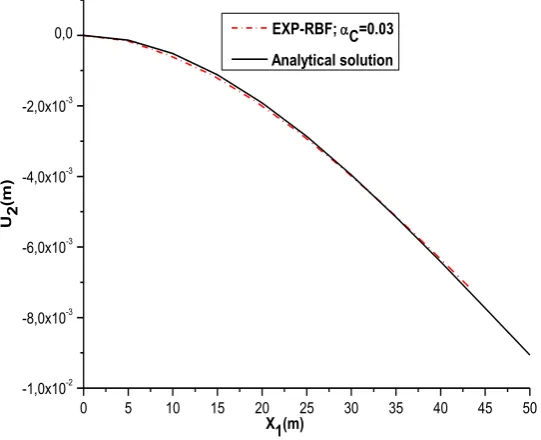
Figure 7 shows the deflection results are plotted as function ofx at₁ x2 0,

for the radial basis RBF-EXP, the number of nodes nt= 55 and the size of the support domain

(_S 5) with the cubic spline function and shape parameters: _c  0.03 to RBF-EXP.

We considered n_t= 55 for which the method is convergent and the value of energy error is low. There is a coincidence between the curves representing the radial basis RBF-EXP of the LRPIM method and the curve of the analytical solution which corresponds to the upper end of the domain of convergence i.e. S between 1.80 and 5.

0 5 10 15 20 25 30 35 40 45 50

-1,0x10-2

-8,0x10-3

-6,0x10-3

-4,0x10-3

-2,0x10-3

0,0

U2

(m

)

X1(m)

EXP-RBF;_C=0.03 Analytical solution

Figure7 Deflections as a function of x₁ at x20 for the radial basis RBF-EXP (nt 55for C 0.03 ) and the analytical solution

Figure 8 Shear stress (₁₂) as function of x at 2 x1 L/2 for the radial basis RBF-EXP and

175

 t

-6 -4 -2 0 2 4 6 -140

-120 -100 -80 -60 -40 -20 0

 



pa

)

RBF-EXP) Analytical solution

x₂(m)

175 nodes

Figure8 ₁₂ as a function of x₂ at x₁ L/2 for the radial RBF-EXP, (n_t 175for _C 0.03 ) and the analytical solution.

5 Conclusion

In this paper the meshless LRPIM method is employed for solving a 2D elastostatic problem. The governing equations depend on the weak form and the partitions of domain. The LRPIM method and its dependency on sizing parameter of S are associated to different

parameters coming out of weak form formulation. We have investigated for _Q 2 the nature

of convergence domain as a function ofS; the effect of number nodes n , by varying nature of t

material and the radial basis functions RBFs, we conclude that for small values of n_t(55)lead to the upper extremity of convergence domain which is limited to _S 5.

For greater value of n (91, 175, 189) we found that the maximal value for convergence domain t

the maximum extremity decreases when n increases, We found _t _S 3.66. No dependency is noted of the maximum extremity value: _S of convergence domain, and the elastic nature of materials.

Conflict of Interests

REFERENCES

[1] O. C. Zienkiewicz, and R. L. Taylor, the Finite Element Method, 5th edition, Butterworth Heinemann, Oxford, UK, 2000.

[2] B. Nayroles, G. Touzot and P. Villon, Generalizing the finite element method:diffuse approximation and diffuse elements, Computational Mechanics, 10 (1992), 307-318.

[3] N. Moës, J. Dolbow and T. Belytschko, A finite element method for crack growth without remeshing, International Journal for Numerical Methods in Engineering, 46 (1999), 131–150.

[4] L. Lucy, A numerical approach to testing the fission hypothesis, Astron. J., 82 (1977), 1013–1024. [5] J. J. Monaghan, An introduction to SPH. Computer Physics Communications, 48 (1988), 89–96.

[6] Liu GR, Liu MB, Smoothed particle hydrodynamics – A meshfree practical method, World Scientific, Singapore, 2003.

[7] T. Belyschko, Y.Y. Lu and L. Gu, Element-free Galerkin methods, Int. J. Numerical Methods, 37 (1994), 229–256.

[8] S. N. Atluri, T. Zhu, A new meshless local Petrov–Galerkin (MLPG) approachs in computational mechanics, Comput Mech, 22 (1998), 117–127.

[9] M. Dehghan, R. Salehi, A meshless local Petrov–Galerkin method for the time-dependent Maxwell equations, Journal of Computational and Applied Mathematics 268 (2014) 93–110.

[10] J.G. Wang and G.R. Liu, on the optimal shape parameters of radial basis functions used for 2-D meshless methods, Comput Methods Appl, Mech. Engrg. 191 (2006) 2611–2630

[11] Liu GR, Yan L, Wang JG, Gu YT, Point interpolation method based on local residual formulation using radial basis functions. Struct Eng Mech 14(6) (2002) 713–732

[12] R.L. Hardy,Theory and applications of the multiquadrics–biharmonic method, Computers and Mathematics with Applications 19 (1990) 163–208.

[13] M.J.D. Powell, The uniform convergence of thin plate splines in two dimensions, Numerical Mathematic 68 (1) (1994) 107–128.

[14] M.A. Golberg, C.S. Chen, H. Bowman, (1999), Some recent results and proposals for the use of radial basis functions in the BEM, Engineering Analysis with Boundary Elements 23 (1999), 285–296.

[15] A. Quarteroni, R. Sacco, F. Saleri, Méthodes Numériques, Algorithmes, analyse et applications, Springer, 2007.

[16] S. P. Timoshenko and J. N. Goodier, Theory of Elasticity,3rdedition, McGraw Hill, 1970.

[17] A. Moussaoui and T. Bouziane, Convergence of MLPG Method for Various Materials of a 2D Problem, Applied Mathematical Sciences, 8 (2014), 3405 - 3418.