in the population sciences published by the Max Planck Institute for Demographic Research Konrad-Zuse Str. 1, D-18057 Rostock · GERMANY www.demographic-research.org
DEMOGRAPHIC RESEARCH
VOLUME 20, ARTICLE 21, PAGES 503-540
PUBLISHED 05 MAY 2009
http://www.demographic-research.org/Volumes/Vol20/21/ DOI: 10.4054/DemRes.2009.20.21
Research Article
The Malawi Diffusion and Ideational Change
Project 2004–06: Data collection, data quality,
and analysis of attrition
Philip Anglewicz, jimi adams, Francis Obare,
Hans-Peter Kohler, and Susan Watkins
This publication is part of the proposed Special Collection “HIV/AIDS in sub-Saharan Africa”, edited by Susan Watkins, Jere Behrman, Hans-Peter Kohler, and Simona Bignami-Van Assche.
© 2009 Philip Anglewicz et al.
This open-access work is published under the terms of the Creative Commons Attribution NonCommercial License 2.0 Germany, which permits use, reproduction & distribution in any medium for non-commercial purposes, provided the original author(s) and source are given credit.
1 Introduction 504
2 Data 504
3 Sample representativeness 506
4 Interviewer effects 507
4.1 Interviewer recruitment and training 508 4.2 Role-restricted interviewer effects 508 4.3 Role-independent interviewer effects 509
5 Response reliability 519
6 Attrition 521
7 Conclusion 530
8 Acknowledgments 531
References 533
The Malawi Diffusion and Ideational Change Project 2004–06:
Data collection, data quality, and analysis of attrition
Philip Anglewicz1 jimi adams2 Francis Obare3 Hans-Peter Kohler4
Susan Watkins5
Abstract
In this paper we evaluate the quality of survey data collected by the Malawi Diffusion and Ideational Change Project by investigating four potential sources of bias: sample representativeness, interviewer effects, response unreliability, and sample attrition. We discuss the results of our analysis and implications of our findings for the collection of data in similar contexts.
1 (PhD) Population Studies Center, University of Pennsylvania, 239 McNeil Building, 3718 Locust Walk,
Philadelphia, PA 19104-6298. Phone: (215) 898-6441. Fax: (215) 898-2124. E-mail: [email protected].
2 (PhD) Robert Wood Johnson Foundation Health and Society Scholars Program, Columbia University.
E-mail: [email protected].
3 (PhD) Population Council, Nairobi, Kenya. E-mail: [email protected].
4 (PhD) Department of Sociology, University of Pennsylvania. E-mail: [email protected]. 5 (PhD) California Center for Population Research, University of California Los Angeles.
1. Introduction
Empirical analysis in demographic publications typically involves hypothesis testing about the determinants and correlates of demographically relevant outcomes. Although high-quality data are essential for these analyses, published articles rarely address important characteristics of the data, such as interviewer effects or, in longitudinal data, the implications of attrition for the results. This paper examines the data quality of the Malawi Diffusion and Ideational Change Project (MDICP), a data set that is widely used for analysis of social networks, HIV/AIDS and family planning in sub-Saharan Africa. We investigate several sources of potential bias in a longitudinal dataset: sample representativeness, interviewer effects, response unreliability, and sample attrition.
The analysis in this paper builds on an earlier evaluation conducted by Bignami et al. (2003). We extend this previous research for several reasons. First, as the MDICP has completed three additional waves since 2003 and now encompasses five waves of data collection (1998, 2001, 2004, 2006, and 2008), some aspects of data quality have become more important. For instance, potential attrition biases may have increased as attrition of the initial cohorts has accumulated across each survey wave, or the addition of new samples of respondents – most importantly a new adolescent sample in 2004 – may have changed the sample properties and representativeness of the survey. To address these issues, we conduct a series of data quality analyses for the MDICP data, including comparisons of the data with the Malawi Demographic and Health Surveys (MDHS) and analyses of interviewer effects, response reliability, and sample attrition. The analyses for this paper are similar to those of Bignami et al. (2003), thus permitting a comparison of data quality issues within the first four waves of the project. We do not include the 2008 data, since they are not yet fully ready for analysis.
2. Data
The MDICP is a longitudinal research project with the overall goals of investigating the multiple processes and influences that contribute to variation in HIV risks in a sub-Saharan African context, identifying prevention strategies for managing risks and assessing the potential effect of HIV risk reduction programs on infection risks and disease dynamics. An unusual feature of the data is information on social networks, which permits examination of the role of social interactions on attitudes related to contraceptive use and family planning, as well as AIDS knowledge and risk behavior.
aged 15–49 years and their husbands. Interviews were completed with 1,541 women (out of a possible 1,790) and 1,065 of their husbands (out of a possible 1,520). In 2001, the first follow-up wave, information was collected from (1) the same respondents, (2) sample members who were not found in 1998, and (3) new spouses of respondents who married again between 1998 and 2001.6
In 2004, the third wave of MDICP data collection, interviews were conducted with the same respondents as in 1998 and 2001, as well as all new spouses of respondents. In addition two new samples were added. First, a sample of approximately 1,500 married and never-married adolescents aged 15–28 years was added in each site,7 for two reasons: to adjust for aging of the 1998 sample over time, which led to under-representation of the adolescent population by 2004; and to introduce never-married adolescents into the MDICP sample (the 1998 sample was restricted to ever-married men and women). These adjustments made the 2004 sample generally representative of the rural population in each sample district. The 2004 adolescent sample yielded completed interviews with 718 female (256 married) and 767 male (409 never-married) respondents.8
Second, in 2004 the MDICP collected biomarkers for HIV, gonorrhea, chlamydia and trichomonas from all consenting respondents.9 Because the administration of such tests required personnel trained in biomarker specimen collection and HIV/STI counseling, the project recruited a team of nurses to provide counseling, collect the biomarkers, and administer a short questionnaire. The additional personnel and time required to complete both the main survey and the biomarker collection necessitated two separate visits to each respondent. As a result there were two data collection teams: the “main survey” and the “biomarker collection” teams. The survey team first administered the main questionnaire. This was followed by the biomarker collection team, which typically visited respondents two or three days after the main survey interview. Also, because HIV and STI tests were conducted in a laboratory in Malawi (as opposed to using rapid results HIV test kits, as MDICP did in 2006 and 2008), test results were given to respondents between two and four months after testing at each fieldwork site.
The 2006 sample comprised the same respondents as in 2004 (main sample of ever-married men and women from 1998, plus the 2004 adolescent sample and all new
6 For more details on the 1998 and 2001 sampling strategy, see Watkins et al. 2003. 7 A description of sampling strategy for the 2004 adolescents can be found at:
http://www.malawi.pop.upenn.edu/Level%203/Malawi/docs/Sampling3.pdf.
8 In the age group 15–24 a smaller proportion of men are married than women because of the higher age at
which men in rural Malawi marry.
9 Protocol for 2004 MDICP biomarker collection by Bignami Van-Assche et al. (2004) can be found on the
spouses in 2006), plus the spouses of the 2004 adolescent sample. Several changes were made to the survey instrument and the composition of the data collection teams in 2006. The team was expanded to include three teams: the “family listing team,” the “main survey team”, and the “biomarker team”. The family listing team first collected detailed information on the family history, transfers among family members, and family mortality for each respondent. This was followed by the main survey team and finally by the biomarker team. As in 2004, the 2006 biomarker team administered a small survey, but due to the relatively low prevalence of gonorrhea, chlamydia and trichomonas found in 2004,10 the project conducted testing for HIV only.11 Respondents in 2006 were given the opportunity to receive their HIV test results immediately after testing.
3. Sample representativeness
One important purpose of population surveys is to make inferences about the larger population from which the survey samples are drawn (Groves and Couper 1998; Levy and Lemeshow 1999). The validity and reliability of the inferences depend on (1) the manner in which the (initial) sample was chosen and, in the case of a longitudinal study, how individuals were followed over time; (2) the participation rate in the survey; and (3) the procedures involved in data collection (Levy and Lemeshow 1999). These factors in turn determine how representative the sample is of a larger population and how valid the summary measures. Although the MDICP was not designed to be representative of the rural population of Malawi (Watkins et al. 2003), we compare the sample characteristics with those of the rural population of Malawi obtained from the nationally representative MDHS. We focus below on basic socio-demographic characteristics (age, educational attainment, and current marital status), fertility and family planning, and knowledge, behavior, and perceptions about HIV/AIDS among the ever-married sample from the 2004 and 2006 survey rounds.
A comparison of the MDICP sample characteristics with those of the rural population of Malawi obtained from the MDHS shows that, with a few exceptions, characteristics of the MDICP sample differ significantly from those obtained from the MDHS (presented in Appendix 1, Tables 1.1–1.3). There are two possible explanations for this pattern. First, these differences could simply be due to sampling variability: that
10 The 2004 MDICP prevalence for chlamydia was 0.3%, 3.1% for gonorrhea, and 2.3% for trichomonas. See
Obare et al. (2008) for additional details regarding 2004 HIV and STI testing and results dissemination.
11 A more detailed description of the 2004 and 2006 MDICP sampling strategies can be found at
is, the fact that the MDICP and the MDHS sampled different subsets of the rural population of Malawi. In particular, the MDHS includes most rural townships as “rural”12, whereas the entire MDICP sample lives in villages. The characteristics of rural townships and villages are likely to differ: for example, a comparison of MDICP prevalence among the adolescent sample in Balaka District with HIV prevalence of adolescents in townships covered in a study by Mensch et al. (2008) shows that prevalence is considerably higher in the townships.13 Alternatively, the difference between the 1998 MDICP and the 2000 MDHS estimates could also be due to temporal changes in the indicators, given that the two surveys were conducted two years apart.
4. Interviewer effects
In this section we use data from MDICP waves 3 and 4 to evaluate two distinct types of interviewer effects: role-restricted and role-independent. Role-restricted interviewer effects refer to the possible influence of an interviewer’s behavior and conduct on survey responses. For example, some interviewers may be more comfortable during interviews and therefore better at obtaining responses to some of the questions considered by many MDICP respondents to be sensitive, such as marital infidelity and suspected spousal infidelity. The background characteristics of each interviewer, which
are role-independent, may also influence survey responses. We therefore test for the
presence of independent effects on MDICP survey responses. We also test for role-independent effects on HIV biomarker collection, by examining whether the gender of the nurse responsible for biomarker collection is associated with accepting HIV testing and receiving test results. Since the gender of the interviewer is a frequent topic of research on interviewer effects (for example, Becker et al. 1995; Blanc and Croft 1992; Verrall 1987; Weinreb 2006), we pay particular attention to the role of interviewers’ and respondents’ gender.
12 Personal communication, Christopher Manyamba, National Statistics Office, Malawi.
13 We are grateful to Paul Hewett of the Population Council for providing us with unpublished tabulations
4.1 Interviewer recruitment and training
In the survey literature, it is typically taken for granted that interviewers from outside the area and of the same gender as the respondent are likely to get more reliable and valid responses on sensitive questions than are local interviewers or cross-gender pairs of interviewer and respondent. The MDICP recruits interviewers from each of the three fieldwork sites, all of whom are secondary school graduates and fluent in English; in addition, for budgetary reasons, the MDICP permits cross-gender interviewing. An analysis of data from the MDICP sister project in Kenya found that “insider” interviewers – defined as interviewers who knew the respondent or his/her family – tend to get more consistent responses from respondents (Weinreb 2006). In the MDICP, for each respondent, the interviewer is asked to report if, and how well, he/she knows the respondent, in addition to a number of other considerations, such as the interviewer’s own concern about the risk of becoming infected with HIV. Unlike our experience in Kenya, very few interviewers in Malawi knew any of the respondents in the MDICP sample.14 Therefore the analysis of insider–outsider interviewer effects is not replicated here. We do, however, examine cross-gender interviewing. All interviewers are given several days of training prior to the start of fieldwork. This training was given by locally hired supervisors who were university graduates with experience with prior waves of the project.
4.2 Role-restricted interviewer effects
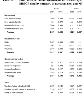
To estimate interviewer effects, we use the interclass correlation coefficient (ρ), the same measure used by Bignami et al. (2003). The interclass correlation coefficient measures the percentage of the total variance for a particular question that is attributable to the interviewer. A zero value for the interclass correlation coefficient would represent no interviewer effect for a particular question. Because there is usually some variance attributable to the interviewer, the survey literature considers acceptable values for the interclass correlation coefficient that are in the range of 0.01–0.07.15
In testing for role-restricted interviewer effects, we examine background characteristics (schooling, economic status), gender norms, and HIV/AIDS perceptions
14 Of men and women interviewed in 2004, less than 5% of interviewers reported knowing respondents “very
well” or “quite well,” the two categories used by Weinreb (2006) to identify “insiders.”
15 As noted in Bignami et al. (2003), a key assumption in calculating the inter-class correlation coefficient is
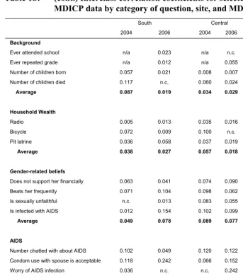
and behaviors. We calculate the ρ separately for men and women, 2004 and 2006, and for each of the three fieldwork sites. The results are presented in Tables 1a and 1b.
Our results show that role-restricted interviewer effects are more evident for questions that our qualitative data suggest are sensitive than for background characteristics. Whereas most ρ values for background characteristics are within the range of 0.01–0.07, many of the ρ values for AIDS and gender-related beliefs questions exceed the 0.07 level. Several of the background variables (for example, presence of a radio) do not exceed the 0.07 level for any site or MDICP wave, and for none of the background questions considered does the percentage of variance attributable to the interviewer’s role exceed 12%. In contrast, several AIDS and gender questions are consistently greater than the 0.07 level, and many of the questions expected to be more sensitive – such as the acceptability of divorcing a spouse with AIDS or using a condom with a spouse – exceed the 0.12 level across gender, site, and MDICP wave, suggesting that these questions are indeed more sensitive. There does not, however, appear to be any systematic variation in role-restricted interviewer effect by site or gender, or across MDICP waves. While the regional average is higher for men from all three MDICP sites in 2006, this is not the case for women.
In summary, we find role-restricted interviewer effects in 2004 and 2006 that are similar to those in 1998 and 2001. Most are in the conventionally acceptable range of 0.01–0.07 for both men and women, although they are markedly higher for questions that, in the Malawian context, appear to be more sensitive.
4.3 Role-independent interviewer effects
Role-independent interviewer effects identify characteristics of the interviewer that may lead to response bias. In this section we examine several characteristics of interviewers for their effect on the same set of background, gender, and AIDS questions from the 2004–06 surveys.
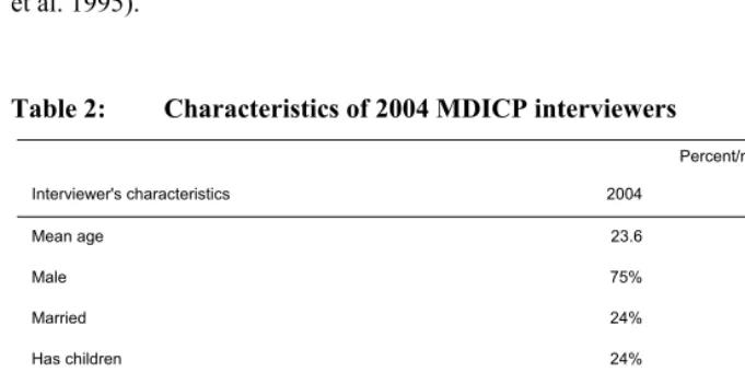
In both waves interviewers responded to a questionnaire that solicited information on their background characteristics. To measure role-independent effects we regress the set of variables used in the previous section on several of the interviewer’s characteristics: age, marital status, gender, having children, home of the interviewer’s mother and father, and perceived likelihood of current HIV infection (summary statistics for MDICP interviewers are displayed in Table 216).
16 As shown in Table 5, not all questions in the interviewer’s questionnaire were asked in both 2004 and 2006.
Table 1a: Interclass correlation coefficients for selected questions in the MDICP data by category of question, site, and MDICP year (women)
South Central North
2004 2006 2004 2006 2004 2006
Background
Ever attended school 0.049 0.000 0.024 0.053 n.c. n.c.
Ever repeated grade n/a 0.079 n/a 0.018 n/a 0.058
Number of children born 0.008 0.003 n.c. 0.010 n.c. n.c.
Number of children died 0.055 0.014 n.c. n.c. n.c. 0.007
Average 0.037 0.024 0.024 0.027 0.033
Household wealth
Radio 0.027 0.004 0.014 n.c. 0.009 n.c.
Bicycle 0.007 n.c. 0.000 n.c. n.c. 0.010
Pit latrine 0.016 0.009 0.053 0.050 0.014 n.c.
Average 0.017 0.007 0.022 0.050 0.012 0.010
Gender-related beliefs
Does not support her financially n.c. 0.077 0.031 0.109 n.c. 0.093
Beats her frequently n.c. 0.032 0.051 0.041 n.c. 0.133
Is sexually unfaithful 0.033 0.127 0.081 0.053 0.099 0.116
Is infected with AIDS 0.075 0.179 0.008 0.136 0.223 0.113
Average 0.054 0.104 0.043 0.085 0.161 0.114
AIDS
Number chatted with about AIDS 0.006 0.126 0.034 0.447 n.c. 0.163
Condom use with spouse is acceptable 0.199 0.217 0.058 0.160 0.034 0.096
Worry of AIDS infection n.c. 0.340 0.035 0.212 n.c. 0.253
Number died of AIDS 0.167 n.c. 0.058 0.132 0.044 n.c.
Best friend had sexual partner 0.175 0.102 0.133 0.080 0.092 0.093
Talked about AIDS with spouse 0.001 0.086 0.034 0.053 n.c. 0.066
Unfaithful to current spouse 0.040 0.093 n.c. 0.025 n.c. 0.028
Suspects spousal infidelity 0.051 0.011 0.034 0.052 0.086 0.040
Average 0.091 0.139 0.055 0.145 0.064 0.106
Regional average 0.061 0.088 0.043 0.102 0.075 0.091
Table 1b: (cont.) Interclass correlation coefficients for selected questions in the MDICP data by category of question, site, and MDICP year (men)
South Central North
2004 2006 2004 2006 2004 2006
Background
Ever attended school n/a 0.023 n/a n.c. n/a 0.015
Ever repeated grade n/a 0.012 n/a 0.055 n/a n.c.
Number of children born 0.057 0.021 0.008 0.007 0.230 0.083
Number of children died 0.117 n.c. 0.060 0.024 0.044 0.009
Average 0.087 0.019 0.034 0.029 0.137 0.036
Household Wealth
Radio 0.005 0.013 0.035 0.016 0.007 0.006
Bicycle 0.072 0.009 0.100 n.c. 0.018 0.000
Pit latrine 0.036 0.058 0.037 0.019 0.075 0.024
Average 0.038 0.027 0.057 0.018 0.033 0.010
Gender-related beliefs
Does not support her financially 0.063 0.041 0.074 0.090 n.c. 0.222
Beats her frequently 0.071 0.104 0.098 0.062 n.c. 0.070
Is sexually unfaithful n.c. 0.013 0.083 0.055 n.c. 0.028
Is infected with AIDS 0.012 0.154 0.102 0.099 0.098 0.056
Average 0.049 0.078 0.089 0.077 0.098 0.094
AIDS
Number chatted with about AIDS 0.102 0.049 0.120 0.122 0.069 n.c.
Condom use with spouse is acceptable 0.118 0.242 0.066 0.152 0.024 0.134
Worry of AIDS infection 0.036 n.c. n.c. 0.242 n.c. 0.155
Number died of AIDS 0.104 n.c. 0.055 0.118 0.010 0.008
Best friend had sexual partner 0.132 0.021 0.095 0.039 0.169 0.066
Talked about AIDS with spouse n.c. 0.008 0.023 0.069 0.275 0.170
Unfaithful to current spouse 0.068 0.017 0.086 0.036 0.083 0.047
Suspects spousal infidelity 0.114 n.c. 0.025 n.c. 0.010 0.025
Average 0.096 0.067 0.067 0.111 0.091 0.086
Regional average 0.074 0.052 0.067 0.075 0.086 0.066
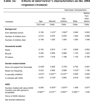
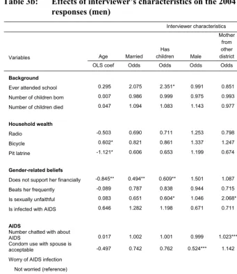
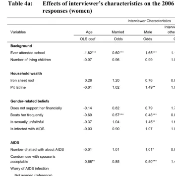
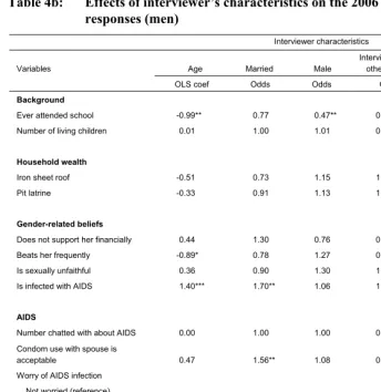
These regressions are estimated separately for male and female respondents. The results are displayed in Tables 3a, 3b, 4a, and 4b.
As with the results for role-restricted effects in Table 1, role-restrictive effects are greater for presumably sensitive questions, such as those concerning gender and AIDS, than for background characteristics. The questions most strongly affected by the interviewer’s characteristics are the acceptability of condom use with a spouse, the number of persons the respondent has chatted with about AIDS, the gender perception variables, and worry of AIDS infection.17 The gender of the interviewer appears to have a stronger effect for female respondents than for male respondents in both 2004 and 2006.
It is interesting to note that an interviewer’s perceived risk of HIV infection is significantly associated with the respondent’s perceptions and beliefs about HIV/AIDS in 2004 and 2006. For example, in 2004 male respondents questioned by interviewers who believed that there was some chance that they were currently HIV positive were more likely to report that they were very worried about HIV than male respondents who were interviewed by male interviewers who did not believe that they themselves were currently HIV positive. Similar strong and highly significant associations are found in the relationship between interviewer’s and respondent’s worry of HIV infection for both men and women in 2006 (Table 4). The significant association between perceived risk of the interviewer and respondent leads to an interesting question regarding the causality of risk perception: is worry of HIV infection for respondents influenced by the perceived risk of the interviewer, or is the perceived risk of an interviewer increased by discussing HIV with numerous respondents who are very worried about infection? Although the answer to this question is beyond the scope of the current study, our results point to the importance of routinely analyzing, and reporting, interviewer effects. Finally we examine the relationship between nurse’s gender and the acceptance of an HIV test and receiving the results of the test. As shown in Table 5, there is little evidence that the gender of the nurse influenced testing acceptance or receiving HIV test results. Across the three MDICP fieldwork sites only female respondents from the northern site who were visited by a male nurse were significantly more likely to return to receive their HIV test results in 2004 than female respondents visited by a female nurse, and male respondents from the southern site who were visited by a male nurse were significantly more likely to refuse HIV testing compared to male respondents visited by a female nurse.
17 Comparing MDICP with MDHS, it is important to note that many of these sensitive questions are either not
Although we do find some effect of background characteristics of interviewers and nurses on survey questions and HIV testing, the results do not decisively identify particular characteristics of interviewers or nurses that are associated with greater response bias. However, as would be expected, one consistent finding is that sensitive survey questions are more responsive to interviewer effects. The results of our analysis are similar to those of Bignami et al. (2003), which also showed consistent influence of particular interviewer characteristics on survey responses. Our results are also consistent with those of a previous study that found stronger interviewer effects for sensitive questions (Blanc and Croft 1992). While our results show some significant effects of interviewer’s gender on survey responses, we do not find any consistent patterns for these effects in our results (for similar results see Verrall 1987 and Becker et al. 1995).
Table 2: Characteristics of 2004 MDICP interviewers
Percent/mean
Interviewer's characteristics 2004 2006
Mean age 23.6 25.1
Male 75% 68%
Married 24% 30%
Has children 24% n/a
Mother from other district 18% n/a
Father from other district 24% n/a
Interviewer from other district n/a 37%
Some likelihood of HIV infection‡ 29% n/a
Some worry of HIV infection* n/a 48%
Table 3a: Effects of interviewer’s characteristics on the 2004 MDICP survey responses (women)
Interviewer characteristics
Variables Age Married
Has
children Male Mother
from other district
Father from other district
Self-assessed
HIV status‡
OLS coef Odds Odds Odds Odds Odds Odds
Background
Ever attended school 0.100 1.512** 1.550** 0.940 0.902 1.272 1.372*
Number of children born -0.012 0.975 0.976 1.002 0.999 1.012 0.998
Number of children died 0.148 1.025 1.004 1.063 1.048 0.990 1.034
Household wealth
Radio -0.102 0.873 1.167 0.856 0.902 0.940 0.953
Bicycle 0.036 0.900 0.868 1.153 1.043 0.966 1.022
Pit latrine -0.475 1.016 1.188 1.144 0.795 0.681** 1.072
Gender-related beliefs
Does not support her financially -0.449* 0.805 0.753* 0.792 0.947 0.954 1.083
Beats her frequently 0.423 0.800 0.899 1.618** 1.195 1.202 0.949
Is sexually unfaithful -0.614* 0.453*** 0.419*** 0.840 0.920 1.284 0.928
Is infected with AIDS 0.070 0.724* 0.805 0.916 1.083 0.797 0.998
AIDS
Number chatted with about AIDS -0.009 0.976** 0.975** 1.006 0.977* 0.988 0.995 Condom use with spouse is
acceptable -0.948*** 0.510*** 0.593*** 0.595*** 1.030 1.558** 0.667***
Worry of AIDS infection
Not worried (reference)
Worried a little 0.117 1.213 1.513* 1.025 1.150 0.927 0.892
Worried a lot -0.554* 0.844 0.903 1.006 1.203 0.498*** 1.218
Don't know worry 0.245 1.271 1.581 0.364** 2.456* 1.451 1.019
Number died of AIDS -0.011 0.987 0.987 0.999 0.997 0.993 1.006
Best friend had sexual partner -0.255 0.719 0.662* 1.074 0.883 0.743 0.922
Talked about AIDS with spouse 0.602 1.061 0.927 1.173 0.823 0.652* 0.674*
Unfaithful to current spouse 1.195* 1.011*** 1.004 1.730 0.988 1.204 0.546
Suspects spousal infidelity 0.360 3.411 2.72** 0.940 0.767 1.474** 1.158
Table 3b: Effects of interviewer’s characteristics on the 2004 MDICP survey responses (men)
Interviewer characteristics
Variables Age Married
Has
children Male
Mother from other district
Father from other district
Self-assessed
HIV status‡
OLS coef Odds Odds Odds Odds Odds Odds
Background
Ever attended school 0.295 2.075 2.351* 0.991 0.851 0.551 2.025**
Number of children born 0.007 0.986 0.999 0.975 0.993 0.991 1.035
Number of children died 0.047 1.094 1.083 1.143 0.977 0.744* 0.896
Household wealth
Radio -0.503 0.690 0.711 1.253 0.798 1.813 0.909
Bicycle 0.602* 0.821 0.861 1.337 1.247 0.863 0.916
Pit latrine -1.121* 0.606 0.653 1.199 0.674 0.724 2.582**
Gender-related beliefs
Does not support her financially -0.845** 0.494** 0.609** 1.501 1.087 0.571* 1.379
Beats her frequently -0.089 0.787 0.838 0.944 0.715 0.569* 0.621*
Is sexually unfaithful 0.083 0.651 0.604* 1.046 2.068* 5.075*** 0.600*
Is infected with AIDS 0.646 1.282 1.198 0.671 0.711 1.367 1.483
AIDS
Number chatted with about
AIDS 0.017 1.002 1.001 0.999 1.023*** 0.956* 1.026***
Condom use with spouse is
acceptable -0.497 0.742 0.762 0.524*** 1.142 1.893** 1.059
Worry of AIDS infection
Not worried (reference)
Worried a little -0.813* 0.607 0.732 0.879 1.190 1.244 1.429
Worried a lot -1.279*** 0.745 0.760 0.592* 1.903** 0.650 2.365***
Don't know worry 0.319 2.200 2.288 1.050 8.279** n/a 3.965
Number died of AIDS 0.035** 1.018* 1.014 0.985 0.990 1.018 1.007
Best friend had sexual partner -0.022 1.250 1.308 1.418 1.409 1.521 0.976
Talked about AIDS with spouse 0.131 1.040 1.108 1.458 0.453* 0.512 1.368
Unfaithful to current spouse 0.899 0.753 0.746 0.637 0.851 1.251 1.249
Suspects spousal infidelity 0.090 1.284 1.168 1.053 0.799 0.382 1.639
Table 4a: Effects of interviewer’s characteristics on the 2006 MDICP survey responses (women)
Interviewer Characteristics
Variables Age Married Male
Interviewer from
other district Worry of HIV
OLS coef Odds Odds Odds Odds
Background
Ever attended school -1.82*** 0.60*** 1.65*** 1.15 0.56***
Number of living children -0.07 0.96 0.99 1.03 1.00
Household wealth
Iron sheet roof 0.28 1.20 0.76 0.86 0.90
Pit latrine -0.01 1.02 1.49** 1.02 0.60**
Gender-related beliefs
Does not support her financially -0.14 0.82 0.79 1.72*** 0.90
Beats her frequently -0.69 0.57*** 0.48*** 0.84 0.83
Is sexually unfaithful -0.37 1.04 1.45** 1.62** 0.90
Is infected with AIDS -0.03 0.90 1.07 1.04 0.99
AIDS
Number chatted with about AIDS -0.01 1.01 1.01* 0.98** 0.98***
Condom use with spouse is
acceptable 0.68** 0.85 0.50*** 1.48*** 1.86***
Worry of AIDS infection
Not worried (reference)
Worried a little -0.19 0.62** 1.05 0.69** 4.58***
Worried a lot 2.38*** 1.59** 0.68** 0.42*** 6.89***
Number died of AIDS -0.06 0.92** 0.98 0.95 0.98
Best friend had sexual partner 0.76 1.49* 1.73*** 0.66* 1.21
Talked about AIDS with spouse 0.17 1.65** 0.77 1.14 1.04
Unfaithful to current spouse -0.51 1.17 0.59 0.86 0.87
Suspects spousal infidelity 0.08 1.86*** 1.53*** 0.88 1.00
Table 4b: Effects of interviewer’s characteristics on the 2006 MDICP survey responses (men)
Interviewer characteristics
Variables Age Married Male
Interviewer from
other district Worry of HIV
OLS coef Odds Odds Odds Odds
Background
Ever attended school -0.99** 0.77 0.47** 0.79 0.69*
Number of living children 0.01 1.00 1.01 0.99 1.00
Household wealth
Iron sheet roof -0.51 0.73 1.15 1.21 0.88
Pit latrine -0.33 0.91 1.13 1.65* 1.17
Gender-related beliefs
Does not support her financially 0.44 1.30 0.76 0.69** 1.08
Beats her frequently -0.89* 0.78 1.27 0.83 0.90
Is sexually unfaithful 0.36 0.90 1.30 1.07 0.71
Is infected with AIDS 1.40*** 1.70** 1.06 1.94*** 2.52***
AIDS
Number chatted with about AIDS 0.00 1.00 1.00 0.99* 0.99
Condom use with spouse is
acceptable 0.47 1.56** 1.08 0.53*** 0.71*
Worry of AIDS infection
Not worried (reference)
Worried a little -0.54 0.68* 1.04 0.98 3.67***
Worried a lot 0.50 1.86** 1.25 0.59** 8.54***
Number died of AIDS -0.06*** 0.96*** 1.00 0.98** 0.97**
Best friend had sexual partner 0.14 1.26 1.08 1.07 1.05
Talked about AIDS with spouse 0.62 1.01 1.09 1.48 1.12
Unfaithful to current spouse 0.83** 1.04 2.09*** 0.91 0.86
Suspects spousal infidelity 0.03 0.95 0.80 1.06 1.16
Table 5: Percentage of respondents accepting HIV test and receiving HIV test results by sex of nurse for each site: MDICP 2004
Gender of nurse
Female Male Total
Women
Refused HIV test
South 8.6% 8.3% 8.5%
Center 10.3 9.5 9.9
North 6.6 5.9 6.5
Received HIV test result
South 74.6 71.6 74.2
Center 80.2 80.2 80.2
North** 56.6 75.4 61.0
Men
Refused HIV test
South* 7.2 13.5 8.9
Center 9.3 7.8 8.2
North 8.0 8.1 8.1
Received HIV test result
South 75.2 73.3 74.8
Center 80.6 80.5 80.5
North 62.2 59.8 61.2
5. Response reliability
A common method of identifying response validity is by testing the reliability of responses across survey waves. Any changes in responses that are predictable across waves (for example, age, level of education, number of children) represent lack of response validity, which can also shed doubt on other survey responses that are not predictable but are critical for research on HIV/AIDS. In this section we compare responses over time, focusing on characteristics that change in a predictable manner: age, level of education (for the respondent and the respondent’s spouse), number of children, and child mortality.18
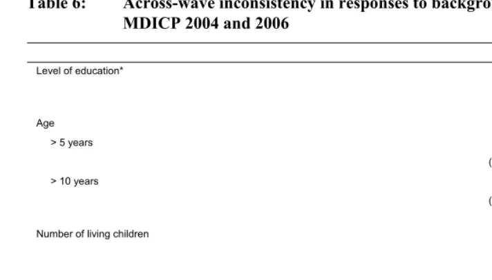
Differences in reporting of background characteristics are found for a substantial percentage of respondents across MDICP data waves, as shown in Table 6. For example, approximately 14% of both men and women report differences in their completed level of education between 2004 and 2006, compared with 9% of respondents who report differences in completed level of education within waves. Similarly, larger reporting discrepancies across waves are found for age: over 10% of men and women reported a greater than five-year difference in their own age between MDICP 2004 and 2006.
We also included tests of reliability across waves for two questions that may be considered sensitive to Malawian respondents: use of family planning and reporting child deaths. Consistency in reporting child death was evaluated by the percentage of respondents reporting a larger number of child deaths in 2004 than in 2006, for those who report having had at least one death. As with reports of the total number of children, men were more inaccurate in reporting children’s death, which probably reflects the greater involvement of rural Malawian women in childbearing and rearing; moreover, men with children out of wedlock may report the deaths of some of them in one survey round but forget them in another.
Overall, the results for cross-wave response consistency are similar to those found by Bignami et al. (2003): inconsistencies in reporting background characteristics vary across waves for 10–15% of MDICP respondents.
18 In Appendix 2, Table 2.1 we also show results for reporting consistency within waves, by comparing
Table 6: Across-wave inconsistency in responses to background variables: MDICP 2004 and 2006
Men Women
Level of education* 14% 13%
(832) (1,290)
Age
> 5 years 13% 12%
(1,118) (1,103)
> 10 years 4% 5%
(1,118) (1,103)
Number of living children 15% 10%
(838) (1,241)
Underreporting child mortality 15% 12%
(1,080) (1,149)
Ever used family planning 11% 10%
(1,096) (1,407)
Note: * Education is measured as a three-category variable: 0 = no school, 1 = completed some primary school, 2 = completed some secondary school.
It is important to note that these inconsistencies occurred despite considerable background data checking and verification in the field. For example, in order to identify the correct respondent to interview, interviewers were given background information for each respondent (as reported from previous waves), including age, marital status, and the names of spouses and parents. In addition several background variables were entered into a database during fieldwork and compared with reports from previous waves. These data checks were used to (1) ensure that the correct respondent was interviewed and (2) verify data entry from the previous wave. The discrepancies in reporting of background characteristics across waves are therefore likely due to differences in reporting by respondents.
6. Attrition
All longitudinal data collection projects face the inherent problem of sample attrition: the failure to find or reinterview individuals who were surveyed in an earlier wave of the study. In rural sub-Saharan Africa rates of attrition are particularly high (Alderman et al. 2001; Bignami-Van Assche, Reniers, and Weinreb 2003; Maluccio 2000). Attrition leads to decrease in sample sizes, which can reduce power in statistical analysis.19 More importantly, however, attrition may bias subsequent analyses if those who leave the sample are substantially and systematically different from those who do not – particularly on unobserved characteristics (Alderman et al. 2001; Fitzgerald, Gottschalk, and Moffitt 1998; Thomas, Frankenberg, and Smith 2000; Ziliak and Kniesner 1998).
Numerous events can lead to sample attrition, including short- or long-term mobility – whether for work, family or other reasons (Ford and Hosegood 2005; Reniers 2001; Reniers 2003), mortality (Doctor and Weinreb 2005; Ford and Hosegood 2005; Grassly et al. 2004; Timaeus and Jasseh 2004), failures to recontact respondents in the absence of reliable addresses, or refusal of respondents to participate in follow-up waves of the study. Tables 7a and 7b present recruitment status and reason for attrition between MDICP waves 3 and 4 (2004–06) for men and women respectively.20 Column 1 represents the full sample and columns 2–4 divide the sample across the three different project sites. Panel A represents figures for the full MDICP sample in 2006, while Panel B displays 2006 outcomes for only those individuals in the sample who were successfully interviewed in 2004.
Table 7 shows that the vast majority of sample loss is due to migration. Men are more likely to leave the sample than women, particularly in the southern site; this is often due to marital instability (Anglewicz 2007; Reniers 2003), combined with the largely matrilocal residential patterns followed in this district. Refusal rates within this study remain remarkably low, due in part to substantial resources allocated to follow-up in the MDICP (Bignami-Van Assche et al. 2003; Watkins et al. 2006; Weinreb, Madhavan, and Stern 1998).
19 While MDICP interviews all new spouses in each wave, the addition of new spouses does not compensate
for the loss of out-migrants. The overall number of out-migrants exceeds the number of in-migrants because individuals leave the MDICP sample area for several reasons (described above), but only enter the sample for one reason: marriage to an MDICP respondent. Also, we find that the characteristics of out-migrants are different from those of in-migrants in some aspects that are relevant to MDICP research (as we indicate below with regards to HIV status).
20 A migration follow-up study was conducted in 2007 in which a team of interviewers attempted to interview
Table 7: 2006 Family listing visit outcomes for all MDICP respondents, and respondents interviewed in 2004
All Respondents Interviewed in 2004
Total Men Women Total Men Women
All Regions
Complete 69.9% 68.2% 71.4% 81.6% 80.8% 82.4%
Refusal 1.2 1.5 0.9 1.4 1.7 1.3
Hospitalized 0.2 0.1 0.3 0.2 0.1 0.3
Dead 2.7 2.9 2.6 1.3 1.5 1.1
Not Found 5.9 6.5 5.3 1.8 1.4 2.1
Temp. Absent 1.7 2.2 1.2 1.2 2.0 0.6
Moved 16.5 16.7 16.4 11.4 11.4 11.3
Other 1.9 1.9 1.9 1.1 1.1 0.9
N 5157 2397 2760 3201 1439 1762
South
Complete 65.5 60.5 70.3 78.6 74.9 81.7
Refusal 1.7 1.8 1.5 2.2 2.0 2.3
Hospitalized 0.3 0.1 0.4 0.2 0.0 0.3
Dead 2.7 3.0 2.4 1.0 1.2 0.8
Not Found 8.6 9.6 8.0 2.5 2.4 2.6
Temp. Absent 2.4 3.7 1.1 2.0 3.5 0.8
Moved 16.9 19.4 14.5 12.5 14.6 10.8
Other 1.9 1.9 1.8 1.0 1.4 0.7
N 1809 899 920 1105 493 612
Center
Complete 73.1 74.2 72.1 80.2 80.4 80.0
Refusal 1.4 2.2 0.7 1.3 2.3 0.5
Hospitalized 0.3 0.1 0.3 0.3 0.2 0.3
Dead 3.8 3.6 3.9 2.0 1.9 2.1
Not Found 1.6 0.6 2.5 1.7 0.6 2.6
Temp. Absent 0.1 0.1 0.1 0.2 0.2 0.2
Moved 18.4 18.0 19.1 13.4 13.3 13.4
Other 1.3 1.2 1.3 0.9 1.1 0.9
N 1618 724 894 1060 474 576
North
Complete 71.5 71.3 71.7 86.2 87.2 85.5
Refusal 0.6 0.6 0.5 0.8 0.6 0.9
Hospitalized 0.1 0.0 0.1 0.0 0.0 0.0
Dead 1.8 2.2 1.5 0.9 1.3 0.5
Not Found 6.9 8.6 5.5 1.1 1.1 1.1
Temp. Absent 2.3 2.3 2.3 1.5 2.3 0.7
Moved 14.3 12.4 15.9 8.2 6.2 10.1
Other 2.5 2.6 2.5 1.3 1.3 1.2
While researchers would ideally like to keep levels of attrition as low as possible, the more important issue is whether those who leave the sample vary systematically from those who remain in the sample. Tables 8a and 8b present descriptive comparisons between these two populations. All variables in Tables 8a and 8b come from the 2004 (wave 3) data and are thus limited to those respondents who were successfully interviewed in 2004.21 Panel A presents the figures for women and Panel B for men.
For both men and women, those who leave the sample had fewer children, were less likely to be from the northern site, where divorce is less common (Reniers 2003), and were less likely to be members of indigenous (African International) churches compared to respondents who were successfully recontacted. Several other differences by recruitment status apply only to men or women. Specifically, women who left the sample were more likely to be younger, to be from Roman Catholic churches, to have achieved higher levels of education, to have used contraception, and to have previously lived outside their current district of residence than are women who were reinterviewed in 2006. Men who left the sample were more likely to be from the southern site and to be Muslims.
HIV status itself is associated with attrition, as shown in Figure 1. Respondents who were HIV positive in 2004 were less likely to be successfully recontacted in 2006. In 2004, biomarker specimens were analyzed in a laboratory and thus were not available immediately (as they were in 2006, when the MDICP used a rapid test). Although results were available subsequently, about a third of those tested did not receive their HIV test results: some perhaps because they had moved, were sick, had died, or were away temporarily; others perhaps because during the interval between testing and the availability of results they changed their mind. We thus examine attrition by whether or not the respondent was aware of his/her test result. We find that HIV-positive individuals were more likely to be lost to follow-up regardless of whether they received their HIV test results or not, as shown in the lower panel of Figure 1.
Table 9 presents the results of a series of logistic regressions predicting attrition between waves 3 and 4 (2004–06). The first column in this table presents the bivariate relationships between the indicated variables (measured in 2004) and attrition status. Only three variables show an association with attrition, with ever used of contraception and obtaining HIV test results in 2004 (either positive or negative) being associated with a lower likelihood of attrition, while testing positive for HIV in 2004 is associated with higher levels of attrition from the sample. Model II presents the results for all
21 We also examined these relationships for variables we expected to be associated with attrition using the full
Table 8a: 2004 descriptive statistics by 2006 recruitment status (women)
Reinterviewed Not reinterviewed Difference
Mean Std Dev Mean Std Dev Mean t-test
Age 35.00 (12.97) 28.96 (11.10) 6.04** 8.09
Region
South 0.34 (0.48) 0.36 (0.48) -0.02 -0.52
Center 0.32 (0.47) 0.38 (0.49) -0.05 -1.80
North 0.33 (0.47) 0.26 (0.44) 0.07* 2.35
Religion
None 0.01 (0.09) 0.00 (0.07) 0.00 0.65
Catholic 0.17 (0.38) 0.26 (0.44) -0.08** -3.03
Muslim 0.27 (0.44) 0.25 (0.43) 0.02 0.68
Missionary Prot. 0.25 (0.43) 0.23 (0.42) 0.02 0.62
AIC 0.15 (0.36) 0.09 (0.29) 0.06* 2.48
Pentecostal 0.09 (0.28) 0.09 (0.28) 0.00 0.00
Other 0.06 (0.24) 0.08 (0.27) -0.02 -1.24
Household owns
Bed with mattress 0.38 (0.49) 0.38 (0.49) 0.01 0.18
Radio 0.74 (0.44) 0.74 (0.44) 0.00 0.06
Bicycle 0.54 (0.50) 0.45 (0.50) 0.09 1.34
Pit latrine 0.91 (0.29) 0.84 (0.37) 0.07 1.57
Education
Secondary 0.07 (0.26) 0.15 (0.36) -0.08** -4.50
Primary 0.66 (0.47) 0.68 (0.47) -0.02 -0.72
None 0.26 (0.44) 0.16 (0.37) 0.10** 3.77
Lived elsewhere 6+ months 0.17 (0.38) 0.28 (0.45) -0.11* -2.06
Number of living children 4.04 (2.24) 3.24 (2.22) 0.80** 4.79
Ever used contraception 0.46 (0.50) 0.37 (0.48) 0.09** 3.04
Lifetime sexual partners 1.88 (1.81) 2.05 (2.19) -0.17 -1.26
AIDS worry
Not worried 0.33 (0.47) 0.34 (0.47) -0.01 -0.34
Worried a little 0.22 (0.42) 0.23 (0.43) -0.01 -0.45
Worried a lot 0.46 (0.50) 0.44 (0.50) 0.02 0.54
N 1,451 82.35% 311 17.65%
Table 8b: 2004 descriptive statistics by 2006 recruitment status (men)
Reinterviewed Not reinterviewed Difference
Mean Std Dev Mean Std Dev Mean t-test
Age 37.95 (15.17) 41.06 (13.54) -3.11** -2.60
Region
South 0.32 (0.47) 0.45 (0.50) -0.13** -4.12
Center 0.33 (0.47) 0.34 (0.47) -0.01 -0.35
North 0.35 (0.48) 0.22 (0.41) 0.14** 4.42
Religion
None 0.02 (0.15) 0.01 (0.11) 0.01 1.09
Catholic 0.19 (0.40) 0.21 (0.41) -0.01 -0.40
Muslim 0.26 (0.44) 0.34 (0.47) -0.08* -2.57
Missionary Prot. 0.21 (0.41) 0.17 (0.37) 0.05 1.61
AIC 0.16 (0.37) 0.10 (0.30) 0.06* 2.50
Pentecostal 0.08 (0.27) 0.11 (0.31) -0.03 -1.42
Other 0.07 (0.26) 0.07 (0.26) 0.00 0.00
Household owns
Bed with mattress 0.27 (0.44) 0.30 (0.46) -0.03 -0.51
Radio 0.76 (0.43) 0.70 (0.46) 0.06 1.19
Bicycle 0.54 (0.50) 0.45 (0.50) 0.09 1.34
Pit latrine 0.90 (0.30) 0.92 (0.27) -0.02 -0.46
Education
Secondary 0.08 (0.26) 0.15 (0.36) -0.08 -4.50
Primary 0.70 (0.46) 0.71 (0.46) -0.01 -0.14
None 0.15 (0.36) 0.21 (0.41) -0.06 -1.52
Lived elsewhere 6+ months 0.24 (0.43) 0.32 (0.47) -0.07 -1.44
Number of living children 5.39 (3.46) 4.45 (3.10) 0.94** 3.38
Ever used contraception 0.42 (0.49) 0.39 (0.49) 0.03 1.03
Lifetime sexual partners 4.40 (5.12) 4.59 (4.80) -0.19 -0.49
AIDS worry
Not worried 0.38 (0.49) 0.35 (0.48) 0.03 1.05
Worried a little 0.25 (0.43) 0.28 (0.45) -0.03 1.00
Worried a lot 0.37 (0.48) 0.37 (0.48) -0.00 -0.14
Na 1,162 80.75% 277 19.25%
predictor variables included simultaneously and shows that those who are somewhat worried about contracting HIV are significantly less likely to be successfully reinterviewed than those who are not worried at all (attrition status is not affected for those who are most worried). In Model III we add the respondent’s HIV test results and whether the respondent received their results, both in 2004, each of which is significantly associated with attrition, in the same direction found in bivariate analyses. Model IV includes all predictor variables together with a series of controls, again showing no substantial linkages between these variables and attrition status. The final model presents all predictor variables, HIV status and receipt of testing results in 2004, and all controls. It shows that the respondents’ HIV status and receipt of test results remain strong significant predictors of attrition, net of other controls.
In the last set of analyses of attrition, we present in Table 10 a series of ordinary least squares (OLS) and logistic regression models predicting several outcomes of particular interest based on the results presented above. We estimate a global interaction of each of four outcomes by attrition status on each of the predictor variables, and present the coefficients and summary statistics for the models (Alderman et al. 2001; Becketti et al. 1988; Bignami-Van Assche et al. 2003). Model I predicts a respondent’s level of “AIDS worry” as an ordered logistic regression, with “Not worried at all” as the omitted category, “Worried a little” and “Worried a lot” as the other categories. Models II and III are OLS regressions predicting, respectively, the number of people (other than their spouse) with whom the respondent has discussed AIDS and the respondent’s reported number of sexual partners. Model IV is a logistic regression predicting whether the respondent has ever used contraception.
Figure 1: Success of re-recruitment (2006) by receipt of HIV test results (2004) and HIV status (2004)
% Reinterviewed in 2006 by Receipt of VCT Results in 2004 40 50 60 70 80 90 100
All Women Men
Yes No % Reinterviewed in 2006 by HIV Status in 2004 40 50 60 70 80 90 100 HI V St at u s w/ re su lt s w/ o re su lt s HI V St at u s w/ re su lt s w/ o re su lt s HI V St at u s w/ re su lt s w/ o re su lt s Positive Negative
All Women Men
Table 9: Logistic regressions predicting attrition status between 2004 and 2006
I Predictor variables individually
II All predictor variables
III All predictor variables, plus VCT/HIV status
IV All predictor variables, plus
controls
V All predictor variables, plus VCT/HIV status
& Controls Odds SE Odds SE Odds SE Odds SE Odds SE
AIDS worry a
Little 1.11 0.13 1.33* 0.19 1.24 0.21 1.35 0.25 1.42 0.31
Lot 1.00 0.11 1.07 0.14 0.86 0.14 1.03 0.17 0.73 0.15
Sexual partners 1.02 0.01 1.01 0.01 1.02 0.02 1.02 0.02 1.04 0.03
Contraception 0.76** 0.07 0.92 0.10 1.02 0.14 0.91 0.13 0.96 0.17
AIDS discussion 1.00 0.00 1.00 0.00 1.00 0.00 1.00 0.00 1.00 0.01
VCT 0.51** 0.05 – 0.00 0.58** -0.08 – 0.00 0.50** 0.09
HIV+ 2.88** 0.45 – 0.00 3.65** -0.68 – 0.00 4.06** 0.94
Region b
South 1.39 0.30 1.58 0.42
North 0.42** 0.10 0.49* 0.14
Female 0.91 0.15 0.79 0.16
Age 0.99 0.01 0.99 0.01
Bed with Mattress 1.27 0.24 1.42 0.31
Bicycle 0.95 0.14 0.95 0.17
Schooling c
Primary school 1.71 0.53 1.11 0.43
Secondary school 1.24 0.23 1.03 0.23
Religion d
Missionary Prot. 0.62* 0.14 0.61 0.17
Muslim 0.65 0.15 0.57* 0.15
African Ind. 0.72 0.18 0.64 0.20
Pentecostal 0.77 0.21 0.83 0.27
Other 0.84 0.28 0.68 0.29
Children 0.96 0.14 0.95 0.17
Lived outside 0.91** 0.03 0.91* 0.04
Constant 0.00 -1.79** 0.12 -1.69** 0.17 -0.82 0.45 0.45 0.57
-2 log likelihood -1128.87 -760.35 -687.34 -481.22
χ2 8.44 65.43 73.21 112.88
Pseudo R2 0.00 0.04 0.05 0.10
N 2590 1985 1791 1418
Table 10: OLS and logit models predicting key outcome variables, conditional on attrition between 2004 and 2006: coefficients and odds ratiosa
I AIDS worry
II # AIDS discussion partners
III Number of sexual partners
IV Used contraception
Coef SE Coef SE Coef SE Coef SE
Southb 0.67** 0.11 -1.15** 0.36 0.28 0.19 -0.38** 0.12
*attrition -0.33 0.28 -0.32 0.92 -0.04 0.48 0.10 0.31
Northb 0.69** 0.12 0.42 0.38 -0.63** 0.20 -0.02 0.13
*attrition -0.42 0.37 1.09 1.21 0.72 0.64 -0.39 0.42
Female 0.25** 0.10 -1.76** 0.33 -2.10** 0.17 -0.07 0.11
*attrition -0.26 0.28 0.04 0.90 -0.07 0.47 0.12 0.31
Age -0.02** 0.00 0.00 0.01 -0.01 0.01 -0.04** 0.01
*attrition -0.01 0.01 0.00 0.04 0.02 0.02 1.01 0.02
Owns bed with mattress 0.04 0.11 0.32 0.36 0.17 0.19 -0.02 0.12
*attrition -0.16 0.24 0.55 1.05 -0.82 0.55 0.19 0.27
Owns bicycle -0.03 0.09 0.06 0.29 -0.10 0.15 0.33** 0.10
*attrition 0.23 0.32 -0.17 0.80 -0.35 0.42 0.38 0.36
Secondary educationc -0.08 0.20 0.82 0.63 0.50 0.33 0.43* 0.22
*attrition -0.81 0.52 -1.08 1.72 -0.93 0.90 0.15 0.60
Primary educationc 0.02 0.12 0.11 0.37 0.22 0.19 0.22 0.13
*attrition -0.41 0.31 2.09* 1.01 -0.36 0.53 -0.14 0.35
Number of living children 0.03 0.02 0.13* 0.06 0.17** 0.03 0.16** 0.02
*attrition 0.07 0.05 -0.15 0.18 -0.23* 0.09 0.05 0.07
Lived outside district 0.03 0.09 0.37 0.30 0.28 0.16 0.15 0.10
*attrition 0.23 0.25 1.24 0.81 0.29 0.43 0.21 0.28
Constant (Cut 1) -0.78**d (0.25) 5.60** (0.79) 3.36** (0.41) 0.85** (0.27)
Constant (Cut 2) 0.27e (0.25)
-2 log likelihood -2307.6 -1458.9
χ2 98.44 168.51
Pseudo R2 0.02 0.05
Adjusted R2 0.05 0.13
Summary effects of attrition
Effect of attrition on constant 0.97 (0.68) 0.20 (1.53) 0.16 (0.22) -0.59 (0.76)
X2 test for joint effects of
attrition on:
Constant and coefficients 8.11 10.60 1.42 6.34
f [0.62] [0.48] [0.17] [0.85]
Coefficients (no constant) 8.15 9.49 1.42 6.31
f [0.70] [0.49] [0.17] [0.79]
N 2,194 2,241 2,217 2,231
In this section we have demonstrated that there are several factors that are differentially associated with respondents’ attrition status, which is consistent with attrition analyses for previous waves of MDICP (Bignami et al. 2003), together with other similar studies (Alderman et al. 2001). However, in the analyses presented here, while those who left the sample differ in a handful of bivariate characteristics, in multivariate analyses the parameter estimates are largely unaffected by changes in the sample due to attrition. This latter finding differs from Bignami et al. (2003), who found several gender-specific significant changes in multivariate parameter estimates by attrition status.22 These differences suggest that the significant relationships between attrition and the model estimates found in the MDICP data were more likely to be due to attrition between initial contact and the first re-recruitment attempts than in subsequent survey waves.
7. Conclusion
Gratifyingly, our results here are similar in most respects to the earlier analysis by Bignami et al. (2003) of data quality in the MDICP surveys of 1998 and 2001, which we interpret as providing support for the validity of our findings across the 2004 and 2006 waves. Two findings, however, are new. First, we find that although those lost to follow-up are different from those who were reinterviewed in several characteristics, attrition does not substantially alter the results of our multivariate analysis, a result similar to the same type of analysis of the project’s longitudinal data in Kenya. Second, in 2004 and 2006 we added new questions to the interviewers’ questionnaire, which turned out to be important in our assessment of data quality. Specifically, we found that the interviewers’ estimates of whether or not they themselves were HIV positive at the time of the survey influenced some of the respondents’ reports, particularly the respondents’ perception of risk of whether or not the respondent was worried about becoming infected with AIDS.
Since sensitive questions about HIV risk perception and behavior are central to MDICP research, as to much other research on AIDS, we believe it is important that interviewer effects are investigated further. A useful next step for examining further the association between perceived HIV risk of the interviewer and the respondent would be to administer the interviewer questionnaire before and after fieldwork in order to
22 We also calculated the estimates presented in Table 10 (we do not have Table 13 in this version of the
examine changes in the perceived risk of interviewers over the course of data collection. Also to avoid any potential interviewer effects, preference in hiring should be given to more experienced interviewers, since such individuals are likely to (1) be more skilled at interviewing and (2) be less influenced by the responses of study participants.
Similarly, the analysis of response reliability should be combined with other methods in order to provide a complete representation of the validity of the data. In this research we examine only consistency in responses, which does not allow us to identify cases where individuals misreport systematically. Instead of examining consistency in self-reports, particularly for responses on sensitive topics (like sexual behavior), a more reliable method of evaluating accuracy of reporting could be to compare self-reports with objective measures. Mensch et al. (2008) compare self-reports of ever having sex with STI biomarkers for young women in rural Malawi and find that approximately 8– 10% of women who claim never to have had sex are infected with an STI. However, objective measures such as STI infection are rare, are often not available for all sensitive questions, and are often limited in their ability to identify reporting error: for example, in the case above for Mensch et al. (2008), some of the girls reporting no sexual activity may not test positive for an STI but still be sexually active, a point the authors acknowledge.
Our results highlight the need for analysts to conduct a careful assessment of the quality of data on AIDS-related attitudes and behaviors, and to report those results routinely, as well as the need for readers to be skeptical of results when analyses of data quality are not reported. We demonstrate in our analysis of interviewer effects that the variables that are subject to the most influence by interviewer characteristic are also those that are central to AIDS research, such as marital infidelity, the number of people spoken to about AIDS, and worry about AIDS infection.
This finding emphasizes the importance of going beyond the standard emphasis on the importance of training by conducting systematic research on interviewing techniques, to improve reporting not only on AIDS but on other topics as well. We also encourage more research on ways to assess the validity of responses: while analyses of interviewer effects and response reliability can indicate problematic questions, they cannot resolve many of the questions that they raise.
8. Acknowledgments
References
Alderman, H., Behrman, J.R., Kohler, H.P., Maluccio, J.A., and Watkins, S.C. (2001). Attrition in Longitudinal Household Survey Data. Demographic Research 5(4): 79-124. doi:10.4054/DemRes.2001.5.4.
Anglewicz, P. (2007). Migration, risk perception and HIV infection in rural Malawi. [Ph.D. Dissertation]. Philadelphia: Graduate Group in Demography, Population Studies Center, University of Pennsylvania.
Becker, S., Feyistan, K., and Makinwa-Adebusoye, P. (1995). The Effect of Sex of Interviewers on the Quality of Data in a Nigerian Family Planning Questionnaire. Studies in Family Planning 26(4): 233-40. doi:10.2307/2137848. Becketti, S., Gould, W., Lillard, L.A., and Welch, F. (1988). The Panel Study of
Income Dynamics after Fourteen Years: An Evaluation. Journal of Labor Economics 6(4): 472-492. doi:10.1086/298192.
Bignami-Van Assche, S., Reniers, G., and Weinreb, A.A. (2003). An Assessment of the KDICP and MDICP Data Quality. Demographic Research S1(2): 31-76.
doi:10.4054/DemRes.2003.S1.2.
Bignami-Van Assche, S. (2003). Are we measuring what we want to measure? Individual consistency in survey response in rural Malawi. Demographic
Research S1(3): 77-108. doi:10.4054/DemRes.2003.S1.3.
Bignami-Van Assche, S., Anglewicz, P., Chao, L.W., Reniers, G., Smith, K., Thornton, R., Watkins, S., and Weinreb, A. (2004). Research Protocol for Collecting STI and Biomarker Samples in Malawi. Philadelphia: Population Studies Center, University of Pennsylvania (SNP working paper no.7).
Blanc, A.K. and Croft, T.N. (1992). The Effect of the Sex of Interviewer on Responses in Fertility Surveys: The Case of Ghana. Paper presented at the annual meeting of the Population Association of America, Denver, Colorado, Apri1 30–May 1, 1992.
Doctor, H.V. and Weinreb, A.A. (2005). Mortality among married men in rural Kenya and Malawi. Journal of African Population Studies 20(2): 165-177.
Ford, K. and Hosegood, V. (2005). AIDS Mortality and the Mobility of Children in Kwazulu Natal, South Africa. Demography 42(4): 757-768.
doi:10.1353/dem.2005.0029.
Grassly, N.C., Morgan, M., Walker, N., Garnett, G., Stanecki, K.A., Stover, J., Brown, T., and Ghys, P.D. (2004). Uncertainty in estimates of HIV/AIDS: The estimation and application of plausibility bounds. Sexually Transmitted Infections 80(Sl): 31-38.
Groves, R.M. and Couper, M.P. (1998). Nonresponse in Household Interview Surveys. New York: John Wiley & Sons, Inc.
Levy, P.S. and Lemeshow, S. (1999). Sampling of Populations: Methods and Applications. New York: John Wiley & Sons, Inc.
Maluccio, J.A. (2000). Attrition in the Kwazulu Natal Income Dynamics Study, 1993-1998. Food Consumption and Nutrition Division. Washington, D.C.: International Food Policy Research Institute. Available at:
http://www.ifpri.org/divs/fcnd/dp/papers/fcndp95.pdf.
Mensch, B.S., Hewett, P.C., and Erulkar, A.S. (2003). The Reporting of Sensitive Behavior by Adolescents: A Methodological Experiment in Kenya. Demography 40(2): 247–268. doi:10.1353/dem.2003.0017.
Mensch, B.S., Hewett, P.C., Gregory, R., and Helleringer, S. (2008). Sexual Behavior and STI/HIV Status among Adolescents in Rural Malawi: An Evaluation of the Effect of Interview Mode on Reporting. Studies in Family Planning 39(4): 321-334. doi:10.1111/j.1728-4465.2008.00178.x.
Miller, K., Zulu, E.M., and Watkins, S.C. (2001). Husband-wife survey responses in Malawi. Studies in Family Planning 32(2): 161-174. doi:10.1111/j.1728-4465.2001.00161.x.
National Statistics Office [Malawi] and ORC Macro. 2001. Malawi Demographic and
Health Survey 2000. Zomba, Malawi and Calverton, Maryland, USA: National
Statistics Office and ORC Macro.
National Statistics Office [Malawi] and ORC Macro. 2005. Malawi Demographic and
Health Survey 2004. Zomba, Malawi and Calverton, Maryland, USA: National
Statistics Office and ORC Macro.
population-based voluntary counseling and testing for HIV in rural Malawi. Sexually Transmitted Infections (published online 16 Oct 2008).
Reniers, G. (2001). The post-migration survival of traditional marriage patterns: Consanguineous marriages among Turks and Moroccans in Belgium. Journal of Comparative Family Studies 32(1):21-36.
Reniers, G. (2003). Divorce and Remarriage in Rural Malawi. Demographic Research S1(1): 175-206. doi:10.4054/DemRes.2003.S1.6.
Thomas, D., Frankenberg, E., and Smith, J.P. (2000). Lost But not Forgotten: Attrition and Follow-up in the Indonesia Family Life Survey. Journal of Human Resources 36: 556-592. doi:10.2307/3069630.
Timaeus, I.M., and Jasseh, M. (2004). Adult Mortality in Sub-Saharan Africa: Evidence from Demographic and Health Surveys. Demography 41(4): 757-772.
doi:10.1353/dem.2004.0037.
Verrall, J. (1987). Recruitment of field staff, pretesting and training. In: Cleland, J. and Scott, C. (eds.). World Fertility Survey: An Assessment. Oxford: Oxford University Press.
Watkins, S., Behrman, J.R., Kohler, H.-P., and Zulu, E.M. (2003). Introduction to “Research on demographic aspects of HIV/AIDS in rural Africa”. Demographic Research S1(1): 1-30. doi:10.4054/DemRes.2003.S1.1.
Watkins, S.C., adams, j., Anglewicz, P., Helleringer, S., Manyamba, C., Mwera, J., Reniers, G., and Weinreb, A. (2006). A Rose by Any Other Name: Identifying Elusive and Eager Would-be Respondents in Longitudinal Data Collection. Philadelphia: Population Studies Center, University of Pennsylvania Working Paper.
Weinreb, A.A. (2006). The Limitations of Stranger-Interviewers in Rural Kenya.
American Sociological Review 71(4):1014-1039.
Weinreb, A.A., Madhavan, S., and Stern, P. (1998). 'The Gift Received Must be
Repaid': Respondents, Researchers and Gifting. Paper presented at the Annual
Meetings of the Eastern Sociological Association. Philadelphia, PA, March 19 1998.
Ziliak, J.P. and Kniesner, T.J. (1998). The Importance of Sample Attrition in Life Cycle Labor Supply Estimation. The Journal of Human Resources 33: 507-530.
Appendices
Appendix 1: Sample representativeness
Table 1.1 Comparison of the MDICP and MDHS respondents with respect
to age
1998 MDICP versus 2000 MDHS
South Central North All sites
Age MDHS
(%)
MDICP (%)
MDHS (%)
MDICP (%)
MDHS (%)
MDICP (%)
MDHS (%)
MDICP (%)
15–19 9.5 6.7** 7.5 4.2** 10.2 5.6** 8.9 5.5**
20–24 13.0 19.3* 21.1 15.0** 21.7 17.2* 22.1 17.0**
25–29 19.8 24.9** 23.5 20.4ns 21.1 20.4ns 21.3 22.0ns
30–34 13.8 15.7ns 14.7 14.1ns 15.1 20.9** 14.3 17.0**
35–39 14.0 15.5ns 13.8 16.7* 12.8 16.1* 13.7 16.0**
40–44 9.7 10.2ns 10.7 13.7* 10.8 10.2ns 10.3 11.5ns
45–49 10.3 7.7* 8.7 15.9** 8.3 8.3ns 9.4 11.0*
Total 100.0 100.0 100.0 100.0 100.0 100.0 100.0 100.0
N 4,987 871 3,570 760 1,655 732 10,212 2,434
2004 MDICP versus 2004 MDHS
15–19 8.5 7.5ns 6.9 4.9* 8.8 5.0** 8.0 5.8**
20–24 23.6 18.2** 23.9 19.3** 22.7 13.0** 23.6 17.0**
25–29 21.4 14.0** 21.9 18.5* 21.0 15.2** 21.5 16.0**
30–34 16.5 17.1ns 17.1 18.3ns 14.0 17.8* 16.4 17.7ns
35–39 11.9 15.3** 11.6 16.4** 12.4 20.1** 11.9 17.2**
40–44 10.2 15.6** 10.4 11.8ns 12.5 17.3** 10.5 14.7**
45–49 7.9 12.3** 8.2 10.8* 8.6 11.6* 8.1 11.6**
Total 100.0 100.0 100.0 100.0 100.0 100.0 100.0 100.0
N 5,269 731 3,858 804 1,220 663 10,347 2,198
Notes:a Ever-married respondents (male and female) aged 15–49 years. Percentages may not add up to exactly 100 in some cases due to rounding. All MDHS figures are for rural areas. Differences between MDHS and MDICP estimates are statistically significant at ** p<0.01; * p<0.05. ns = not significant.