Completely Recursive Least Squares and Its Applications

University of New Orleans University of New Orleans

ScholarWorks@UNO

ScholarWorks@UNO

University of New Orleans Theses and

Dissertations Dissertations and Theses

Summer 8-2-2012

Completely Recursive Least Squares and Its Applications

Completely Recursive Least Squares and Its Applications

Xiaomeng Bian

University of New Orleans, xiaomeng.bian@gmail.com

Follow this and additional works at: https://scholarworks.uno.edu/td

Part of the Power and Energy Commons, and the Signal Processing Commons

Recommended Citation Recommended Citation

Bian, Xiaomeng, "Completely Recursive Least Squares and Its Applications" (2012). University of New Orleans Theses and Dissertations. 1518.

https://scholarworks.uno.edu/td/1518

This Dissertation is protected by copyright and/or related rights. It has been brought to you by ScholarWorks@UNO with permission from the rights-holder(s). You are free to use this Dissertation in any way that is permitted by the copyright and related rights legislation that applies to your use. For other uses you need to obtain permission from the rights-holder(s) directly, unless additional rights are indicated by a Creative Commons license in the record and/ or on the work itself.

Completely Recursive Least Squares and Its Applications

A Dissertation

Submitted to the Graduate Faculty of the University of New Orleans in partial fulfillment of the requirements for the degree of

Doctor of Philosophy In

Engineering and Applied Science Electrical Engineering

by

Xiaomeng Bian

B. S. Zhejiang University, China, 2000

Dedication

Acknowledgement

First, I would like to give my sincere thanks to my families: my parents, uncles and aunties, brothers and sisters, and my in-heaven grandparents. Their selfless love and firm support encourage me to face all the challenges in my study-and-life time.

I would like to give my sincere thanks to Dr. George E. Ioup, Dr. Linxiong Li, Dr. Vesselin P. Jilkov, Dr. Huimin Chen and Dr. Zhide Fang for the helpful guidance, suggestions and comments, as well as the patience and time that you have provided. I would express my gratitude to Professor Jiaju Qiu, Professor Deqiang Gan and Professor Meiqin Liu from Zhejiang University, China. I do appreciate your kind instructions and encouragements in the past years. I would also say special thanks to Dr. Huimin Chen for your insightful discussions and comments on my papers and dissertation.

I would also like to express my gratitude to Dr. Ming Yang, Dr. Zhansheng Duan, Dr. Ryan R. Pitre, Mr. Arther G Butz, Mr. Yu Liu, Mr. Rastin Rastgoufard, Mr. Jiande Wu, Mr. Gang Liu, Dr. Bingjian Wang, Dr. Liping Yan, Miss Jing Hou and all the other colleagues and classmates I have met. I do enjoy the “attacking” atmosphere in our Information & System Lab. Your challenging questions do help me refine and improve my ideas.

Table of Contents

List of Figures ... viii

List of Tables ... ix

Abstract ... x

1. Introduction and Literature Review ...001

1.1 Classification of LS, WLS and GLS ...001

1.2 Review of Batch LS/WLS/GLS Solutions...002

1.2.1 Batch LS/WLS Methods ...002

1.2.2 Batch GLS and LE-Constrained LS solutions ...008

1.3 Recursive LS Approaches ...009

1.3.1 Recursive Methods...009

1.3.2 RLS Initialization and Deficient-Rank Problems ...011

1.4 Completely Recursive Least Squares (CRLS) ...014

1.5 CRLS, LMMSE and KF...015

1.6 Power System State Estimation and Parameter Estimation ...016

1.7 Our Work and Novelty ...017

1.8 Outline...021

Nomenclature in Chapters 2-3 ...022

2. Completely Recursive Least Squares—Part I: Unified Recursive Solutions to GLS ...024

2.1 Background ...024

2.2 Problem Formulation ...026

2.3 Theoretical Support ...027

2.3.1 Preliminaries ...027

2.3.2 Recursive solutions to unconstrained GLS ...028

2.3.3 Recursive solutions to LE-constrained GLS ...031

2.3.4 Recursive imposition of LE constraints ...032

2.3.5 Recursive solution to coarse GLS ...035

2.4 Unified Procedures and Algorithms...042

2.5 Performance analysis ...045

2.6 Appendix 046 2.6.1 Appendix A: Proof of Proposition 1...046

2.6.2 Appendix B: Proof of Theorem 1...047

2.6.3 Appendix C: Proof of Fact 4 ...049

2.6.4 Appendix D: Proof of Theorem 2...050

2.6.5 Appendix E: Proof of Theorem 3 ...051

2.6.6 Appendix F: Proof of Proposition 2 ...053

2.6.7 Appendix G: Proof of Proposition 3...053

Imposition and Deficient-Rank Processing...055

3.1 Introduction ...055

3.1.1 Background ...055

3.1.2 Our Work ...056

3.2 Problem Formulations ...057

3.2.1 WLS and Its Batch Solutions ...057

3.2.2 RLS Solutions ...059

3.2.3 Our Goals ...059

3.3 Derivations and Developments ...060

3.3.1 Preliminaries ...060

3.3.2 Development of Recursive Initialization ...060

3.3.3 Deficient-Rank Processing...068

3.4 Overall Algorithm and Implementation ...070

3.5 Performance Analysis...072

3.6 Appendices ...074

3.6.1 Appendix A: Proof of Theorem 2 ...074

3.6.2 Appendix B: Proof of Theorem 5...076

3.6.3 Appendix C: Proof of Theorem 6...078

4. Linear Minimum Mean-Square Error Estimator and Unified Recursive GLS ...079

4.1 Review of LMMSE Estimation and GLS ...079

4.1.1 LMMSE Estimator ...079

4.1.2 LMMSE Estimation Based on Linear Data Model ...080

4.2 Verification of Generic Optimal Kalman Filter ...082

Nomenclature in Chapters 5-6 ...087

5. Joint Estimation of State and Parameter with Synchrophasors—Part I: State Tracking ...088

5.1 Introduction ...088

5.1.1 Background and Motivation...088

5.1.2 Literature Review ...089

5.1.3 Our Work...089

5.2 Formulation and State-Space Models ...090

5.2.1 State Tracking with Uncertain Parameters ...091

5.2.2 Prediction Model for State Tracking...091

5.2.3 Measurement Model of State Tracking...092

5.3 Adaptive Tracking of State...093

5.3.1 Basic Filter Conditioned on Correlation ...093

5.3.2 Detection and Estimation of Abrupt Change in State ...095

5.4 Procedure and Performance Analysis...096

5.4.1 Explanations on Prediction and Measurement Models ...096

5.4.2 Implementation Issues...098

5.4.3 On Observability, Bad-Data Processing and Accuracy ...099

5.6 Conclusions ...106

5.7 Appendices ...106

5.7.1 Appendix A: Derivation of Filter on Correlated Errors and Noise ...106

5.7.2 Appendix B: Derivation of Abrupt Change Estimation ...109

6. Joint Estimation of State and Parameter with Synchrophasors—Part II: Para. Tracking ....111

6.1 Introduction ...111

6.1.1 Previous Work ...111

6.1.2 Our Contributions...112

6.2 Parameter Estimation ...113

6.3 Formulation of Parameter Tracking ...114

6.3.1 Prediction Model ...115

6.3.2 Measurement Model...115

6.4 Tracking of Line Parameters ...116

6.4.1 Basic Filter ...116

6.4.2 Adjustment of Transition Matrix ...118

6.5 Error Evolution and Correlation Calculation ...119

6.6 Procedures and Performance Analysis...122

6.6.1 Parameter Tracking and Overall Procedure ...122

6.6.2 Accuracy and Complexity...122

6.6.3 A Practical Scheme ...123

6.7 Simulations...124

6.7.1 Comparisons with Other Approaches ...124

6.7.2 Practical Two-Step Implementation of the Approach...126

6.8 Conclusions ...128

6.9 Appendix ...128

7. Summary and Future Work ...130

References ...133

List of Figures

Fig. 5.1 State tracking procedure with abrupt-change detection...099

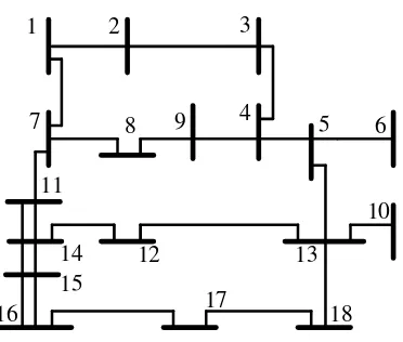
Fig. 5.2 Realistic 18-bus system ...101

Fig. 5.3 Comparison on effect of parameter uncertainty...103

Fig. 5.4 Comparison on effect of abrupt-state-change detection ...105

Fig. 5.5 Comparison with random-walk model ...105

Fig. 5.6 Comparison with forecasting model ...106

Fig. 6.1 Joint state and parameter estimation procedure ...123

Fig. 6.2 12-bus 500kV system...125

Fig. 6.3 Performance comparison with EKF...126

Fig. 6.4 Practical scheme based on 12-bus system ...127

List of Tables

TABLE 5.1 Brach Parameter (18-Bus System) ...103

TABLE 5.2 RMSEs of First Experiment ...104

TABLE 5.3 RMSEs of Secon Experiment ...104

Abstract

The matrix-inversion-lemma based recursive least squares (RLS) approach is of a recursive form and free of matrix inversion, and has excellent performance regarding computation and memory in solving the classic least-squares (LS) problem. It is important to generalize RLS for generalized LS (GLS) problem. It is also of value to develop an efficient initialization for any RLS algorithm.

In Chapter 2, we develop a unified RLS procedure to solve the unconstrained/linear-equality (LE) constrained GLS. We also show that the LE constraint is in essence a set of special error-free observations and further consider the GLS with implicit LE constraint in observations (ILE-constrained GLS).

Chapter 3 treats the RLS initialization-related issues, including rank check, a convenient method to compute the involved matrix inverse/pseudoinverse, and resolution of underdetermined systems. Based on auxiliary-observations, the RLS recursion can start from the first real observation and possible LE constraints are also imposed recursively. The rank of the system is checked implicitly. If the rank is deficient, a set of refined non-redundant observations is determined alternatively.

In Chapter 4, base on [Li07], we show that the linear minimum mean square error (LMMSE) estimator, as well as the optimal Kalman filter (KF) considering various correlations, can be calculated from solving an equivalent GLS using the unified RLS.

Chapter 1: Introduction and Literature Review

1.1 Classification of Linear LS, WLS and GLS

The principle of least squares (LS), which was first invented independently by a few scientists and mathematicians such as C. F. Gauss, A. M. Legendre and R. Adrain [Stigler86][Li07], is a classic and standard approach to obtaining the optimal solution of an overdetermined system to minimize the sum of squared residuals.

The most popular and important interpretation of the LS approach is from the application in data fitting. That is, the best fitting in the LS sense is to approximate a set of parameters (estimands) such that the sum of squared residuals is minimized, where the residuals are differences between the measured observation values and the corresponding fitted ones [Wiki01]. In addition, the LS problem also has various names in different disciplines [Li07]. For instance, in some mathematical areas, LS may be treated as a special minimum l2-norm problem [Bjorck96]. In statistics, it is also formulated as a probabilistic problem widely used in regression analysis or correlation analysis [Freedman05] [Kleinbaum07]. In engineering, it is a powerful tool adopted in parameter estimation, filtering, system identification, and so on [Sorenson80] [Ba-Shalom01]. In particular, in the area of estimation, the LS formulation can be derived from the maximum-likelihood (ML) criterion if the observation errors are normally distributed. The LS estimator can also be treated as a moment estimator [Wiki01].

Roughly speaking, LS problems can be classified into linear and nonlinear cases, depending on whether the involved observation quantities are linear functions of the estimand or not. It is also well known that, with linearization techniques such as Gauss-Newton methods, a nonlinear LS problem may be converted to linearized iterative refinements. This dissertation focuses on linear LS solutions.

largely categorized from the simple to the complex as LS, weighted LS (WLS), and generalized LS (GLS), where linear-equality (LE) constraints may be imposed. Note that in this dissertation the concept of WLS is limited to the case with a diagonal matrix while the GLS has a non-diagonal weighting matrix [Amemiya85] [Greene00] [Wiki02]. In addition, linear-inequality constraints may also be involved and can be treated as combinations of LE constraints [Lawson95].

Note that in some statistics books, “weighted least squares” may be used for LS problems with equal weights while those with distinguished weights are named generally- weighted least squares. As the equally-weighted LS and the conventional LS has the same solution plus mutually-proportional estimation-error covariances, we ignore their difference and follow the convention in [Lawson95] [Bjorck96]: WLS is for LS with distinguished (not all-equal) weights and GLS is for LS weighted by an arbitrary PD matrix.

In summary, we use the following LS/WLS categorizing list to present the LS solutions from simplest to most complex problem setup:

Unconstrained LS LE-constrained LS

Unconstrained/LE-constrained WLS

Unconstrained GLS LE-constrained GLS

Implicitly-LE-constrained (ILE-constrained) GLS

We focus on the development of the recursive unconstrained/LE-constrained/ ILE-constrained LS/WLS/GLS solutions and the related initialization as well as deficient-rank processing. The study starts from the conventional RLS and its exact initializations, which are reviewed below.

1.2 Review of Batch LS/WLS/GLS Solutions

1.2.1 Batch LS/WLS Methods

as [Lawson95] and [Bjorck96]. Among the exiting LS methods and topics, we will review those issues related to our research in detail. Roughly speaking, the (unconstrained) linear LS approach is to solve the following classic (unconstrained) linear LS problem:

ˆ =arg minJ

x

x (1.1a)

with

1( ) ( ) ( ) ( )

M _{T T}

m m m m

m

J z H z H

=

=

∑

where x=[Lx_nL]T _{, [} T _]T m

H

=

H L L _{, and [ ]}T

m

z

=

z L L _. x_n is thenth to-be-determined

quantity. Hmand zmare the coefficient (row vector) and value of the mth observation,

respectively, andM is the total observation number. Typically, xˆ can be obtained via normal-equation solution, QR-decomposition (ofH), Gauss elimination and so on. These methods are reviewed as follows.

The solutions can come from solving the following normal equation:

ˆ

(H H xT ) =H zT (1.2a)

That is,

1 ˆ 1

( M T_{m m}) M _mT _m m= H H = m= H z

∑

∑

Clearly, if and only if (iff)rank( )H =N , (1.2b) has a unique solution and the batch solution is

1

( )

ˆ T

T −  =

 

= 

C H H

x CH z (1.2c)

where estimation-error-covariance-like (EEC-like) matrixCis closely related to the covariance of estimation errors in engineering applications. Matrix triangularization and diagonalization techniques such as Cholesky decomposition (LLT decomposition) can be used to decompose

T

H H and thus compute C and xˆ efficiently [Martin&Wilkinson65] [Passino98], where

the symmetric structure of T

Actually, xˆ can also be determined directly from the nonsymmetric linear equation Hx=z. Gauss elimination with partial pivoting is used to solve Hx=z , and different Gauss-elimination based methods are surveyed in [Nobel73]. Among the existing approaches, the Peters-Wikinson method is a uniform one. It utilizes the LU factorization to reduce the original LS problem to a simplified one with a lower triangular coefficient. Because the solution is obtained from the triangularized coefficient and thus suffers less from rounding error, this method is numerically more stable than those using the normal equation directly. More popularly, the QR decomposition can be employed to decompose the observation coefficient matrix into a product of an orthogonal square matrixQand an upper triangular matrix such that

0 T

T T

 

= _{ }

H Q R (1.3)

where R is an upper triangular square matrix. Correspondingly, the observation-value vectorzis transformed into

1 2

T T T

 

= _{ }

z Q z z% % _(1.4)

Accordingly, the objective function in (1.1a) becomes as simple as

( 1 ) ( 1 ) 2 2

T T

J = z% −Rx z% −Rx +z z% % _(1.5)

Thenxˆcan be obtained conveniently by solving the following linear equation

1

ˆ =

Rx z% _(1.6)

The solution can take advantage of the upper-triangular structure ofRand can be obtained by back substitution efficiently. Accordingly, the computational complexity of solving (1.6), which is denoted by the number of the involved floating-point operations (flops), is only as

low as O N( 2)(order of 2

N ). The computation accuracy is also high because the observation-

For instance, in the Householder transformation based method [Golub65a] [Householder58], the orthogonal matrixQis constructed as a product of a sequence of orthogonal matrix:

1 k N

=

Q Q LQ LQ _(1.7)

whereQ_k =diag(I_{N k−} ,Q%_k). Q%_kis a Householder reflection matrix which is designed to satisfy

2[1 0 1 2 0 1]

T

k k = k N k− +

Q a% % a% L _(1.8)

and a%k is a subvector in the kth column of the following transformed intermediate

observation-coefficient matrix:

[

]

Q Q H

0 a L % (1.9) Consequently, 2 2

2 T /

k = − k k k

Q% I b b b (1.10)

with 2[1 0 1 2 0 1]

T k = k− k N k− +

b a% a% L _.

In the Givens rotation based method [Givens58], the QRD matrixQis a product of a series of plane-rotation matrices which have a specific form as

1

2

3

cos sin

0 sin 0 cos

0 0 θ θ θ θ         =  ₋       

I 0 0 0 0

0 0 0

Q 0 0 I 0 0

0

0 0 I

%

(1.11)

Given a vectora%_{which has the same size asQ}% _{’s column and}

1 1 2 2 3

[ T a T a T T] =

a% a % a % a _{, one has}

a′ =Qa% %=[a₁T cosa%₁ θ +a%₂sin θ a₂T −a%₁sinθ+a%₂cos θ aT T₃] _(1.12)

It is clear that, if 2 2

2 1 2

sinθ =a% a% +a% and 2 2

1 1 2

sinθ =a% a% +a% , then

2 2

1 1 2 2 3

[ T a a T 0 T T]

′ = +

a a % % a a _(1.13)

rotation methods are also developed [Gentleman73] [Hammarling74] [Lawson79], where the multiplication number is reduced by adopting the scaled two-factor form ofH. Owing to the effect of scaling-factor update, the traditional fast rotations may suffer from underflow problems. Correspondingly, self-scaling fast rotations, which can monitor and rescale the size of the scaling factors, are developed in [Anda94] to overcome the underflow problems.

Both the Householder-transformation based and the Givens-rotation based approaches have good properties regarding computation and storage. For instance, the standard Householder

factorization requires 2( 1 ) 3

N M − N flops while the normal-equation method may use

2

1 1

( )

2N M +3N flops. Hence, the Householder transformation method requires roughly the same computation as the LLT decomposition based normal-equation one for M ≈N but has twice computation for M N [Bjorck96]. The standard Givens-rotation method takes more

computation as 2 2( 1 ) 3

N M − N multiplications. However, the QR-decomposition methods

have overwhelmingly higher accuracy than the normal-equation ones. They are numerically

more stable since the solution does not involve ( T )

H H but is determined fromHx=zdirectly.

The Givens rotations are easy to implement and also have convenient recursive forms (see next subsection).

As surveyed in [Lawson95] [Bjorck96], Gram-Schmidt orthogonalization is also employed to produce the orthogonal matrixQin the QR decomposition. The classic Gram-Schmidt method, which first appeared in [Schmidt1908], may lose orthogonality in some ill-conditions and is thus a theoretical tool rather than a good base for numerical algorithms. However, the modified Gram-Schmidt methods can reduce the risk of loss of orthogonality [Gulliksson95]. In addition, the singular value decomposition (SVD) can also be adopted to solve the LS problems. That is, for the LS problem in (1.1), given the SVD ofHas

T

 

=  

 

Σ 0

H U V

0 0 (1.14)

1

0 ˆ

0 0

T −

+  

= _{=  }

 

Σ

x H z V U z (1.15)

where superscript “+” stands for the Moore-Penrose pseudo inverse (MP inverse).

H

1

diag(σ , ,σ_N ) =

Σ L _,

i

σ is the square root of theitheignvalue ofH HT , and rank( )H =N_H.

The left and right singular vectors, which are stored in the orthogonal matrices UandV, are

the corresponding eignvectors ofH HT andHHT, respectively [Lawson95]. The first stable algorithm based on SVD was presented in [Golub65b], where H is reduced to a bidiagonal matrix via Householder transformation of a Lanczos process such that the singular values and vectors refer to eignvalues and eignvectors of a special tridiagonal matrix [Bjorck96]. Later, adaptation and improvement are made to the QR algorithm [Golub68] [Golub70]. Newer Jacobi methods are also developed to improve the relative computation accuracy of the singular values in bidiagonal matrices [Kogbetliantz55] [Hestenes58]. Note that, in (1.14),

H

N ≤N. IfN_H <N, the SVD based solution leads to the minimum-norm LS solution, which is

a powerful tool for the deficient-rank analysis discussed in Sec. 1.3.2.

WLS is generalized from LS, in which each observation is assigned a positive weight: ˆ =arg minJ

x

x (1.16)

with

1( ) ( ) ( ) ( )

M _{T T}

m m m m m

m

J =

∑

Equivalently, ( )T ( )

J = z−Hx W z−Hx , (1.17b)

whereW=diag(L, w_m,L) _(1.17c)

Theoretically speaking, sincew_mcan be easily decomposed into 12 12

m m

w w , problem (1.16) can be

1.2.2 Batch GLS and LE-Constrained LS Solutions

Compared with WLS, GLS is a further generalized LS problem, where the weight W can be an arbitrary positive definite (PD) matrix. Since a GLS problem can always be converted to an equivalent LS form by decomposingW, those methods used for solving LS are all applicable to GLS. For instance, the normal equation of GLS is

ˆ

( T ) ₌ T

H WH x H Wz (1.18)

where (H WHT ) remains symmetric. Then those normal-equation based methods used in LS,

such as LLT decomposition based ones, can still be utilized.

Methods based on the decomposition ofWare also widely adopted. That is,

₌ T

W WW% % (1.19)

Based on (1.19), generalized QRD and SVD methods are developed, where the subsequent

decompositions ofHandW% are performed separately to achieve better numerical accuracy

[Paige90] [Van76]. References [Anderson91], [De92] and [Paige81] further discuss the implementation, application and extension of these generalized methods. In addition, how to

decomposeWinto the symmetric form (1.19) is also an issue. In principle, W% can be the

square root ofW, which is unique sinceWis PD. The square root can be obtained by orthogonal decomposition, Jordan decomposition, Denman-Beavers iteration, the Babylonian

method and so on [Higham86]. Particularly, W% can also be a lower triangular matrix.

Choleksy decomposition can be used. The computation can utilizeW% ’s triangular structure.

In addition, in practical applications, constraints may be imposed to the LS solutions. For example, in curve fitting, inequality constraints related to monotonicity, nonnegativety, and convexity and equality constraints related to continuity and smoothness may be involved [Zhu&Li07]. In the category of linear LS, linear-equality (LE) constrained problems are widely investigated, in which problem (1.1) is subject to a set of consistent LE constraints as

=

with _A∈ NA×N _{and (without loss of generality)}

A

rank( )A =N . One natural way to handle

the LE-constrained LS is direct elimination, with whichxis reduced to a lower dimensional

vector since the constraints imply thatN_Acomponents ofxare always linear combinations of

the leftN−N_A. Correspondingly, the original problem is then converted to an unconstrained

LS problem with reduced dimensions equivalently [Bjorck67] [Lawson95]. The most popular practical methods to solve LE-constrained problems are based on the introduction of Lagrange multiplier [Chong07]. The weighting method is also widely adopted, where each LE constraint is treated as an observation with a “huge” weight [Anda96]. Although this method is very easy to implement, it may lead to poor numerical condition. The LE-constrained LS solution can also be obtained using the null-space method [Leringe70], based on which the close form of the solution can be:

ˆ = +B+[ ( − + )] (+ − + )

x A H I A A z HA B (1.21)

whereA+stands for the Moore Penrose generalized inverse ofA. If rank([A HT T T] )=N ,

(1.21) is the unique solution; otherwise, (1.21) leads to the minimum-norm solution in rank-deficient problems [Wei92a] [Wei92b]. [Zhu&Li07] gives another null-space based form as in (24), which is a useful tool for the subsequent derivations in this dissertation. In addition, other techniques, such as the generalized SVD [Van85], are also introduced to solve and analyze the LE-constrained LS problem. In this dissertation, our purpose is to develop completely recursive LS which provides solutions (theoretically) identical to the batch ones. The above batch methods will provide a solid foundation for the subsequent development.

1.3 Recursive Approaches

1.3.1 Recursive Methods

In those observation-coefficient-matrix decomposition based methods, recursive procedures mainly aim to construct the orthogonal matrixQrecursively [Gill74]. For instance, in the Givens-rotation QRD methods, the rotations of the new observation coefficient can naturally take advantage of the existing upper triangular matrix, where the computation complexity is at

2

( )

O N per cycle [Yang92]. The Gram-Schmidt decomposition can also be performed

recursively in a stable way with O MN( ) per-cycle computational operations [Daniel76]. The

recursion is still applicable to SVD, but the updating computation requires O MN( 2) flops at

each cycle [Bunch78], which is too much compared with recursive Givens rotation and Gram-Schmidt orthogonalization.

Particularly, the matrix-inversion (MI) lemma based RLS, which is a recursive normal-equation method, can obtain C(andxˆ) in another sequential way [Woodbury50] [Chen85]. We will further investigate the MI-lemma-based RLS and generalize it to solve GLS problems. The proposed recursive GLS (RGLS) techniques are also applicable to the QRD-RLS.

Concretely, initialized by

0

0 0 0

1 1

( M T ) ( T )

M _m H Hm m M M

− ′ ′

′=

=

∑

C H H (1.22)

the EEC-like matrixCof the unconstrained LS problem (1.2c) can be computed exactly by the following recursion cycle:

1

1 1 ( 1 1) 1

T T

m m m Hm Hm m Hm Hm m

−

− − − −

= − +

C C C C C (1.23)

whereM₀is the number of initial observations and the recursion/data index m>M₀. ˆx_mcan

be calculated concurrently.

Furthermore, when a set of consistent LE constraints as in (1.20) is imposed, the unique

solution exists iff rank([ T T T] )

N =

A H :

1 1

[ ( ) ]

ˆ ( )

M

T T T

m m m

T

H H −

=

+ +

 =  

= + −



∑

C U U U U

x A B CH z HA B

where H=H_M =[H₁T L H_MT ]T _,

1

[ ]T

M z zM

= =

z z L _{, U satisfies [ ][ ]}T ₌

U U U U% % I and

col( )U% =col(AT) [Zhu&Li07]. Here “col( )X ” denotes the space spanned by all the columns

ofX. Reference [Zhu&Li07] also shows that, the recursion formula in (1.23) is still applicable for the LE case once the LE constraint (1.20) has been imposed on the initialization appropriately. For instance, the recursion procedure for the EEC-like matrix should be initialized as

0

0

1 1

[ T( M T ) ] T

M _m H Hm m

− ′ ′ ′=

=

∑

C U U U U (1.25)

where the iff condition

0

rank([A HT T_M ] )T =N is implicitly satisfied.

In addition, fast RLS methods are also developed [Ljung78] [Cioffi84], where the computation is reduced from some convenient properties of the data, such as the involved matrices’ Toeplitz structure.

The RLS is particularly suitable for real-time applications since sequential algebraic operations at each cycle require low computation as well as fixed storage [Zhou02]. It has been widely applied to such areas as signal processing, control and communication [Mikeles07]. In adaptive-filtering applications, “RLS algorithms” are even referred in particular to RLS-based algorithms for problems with fading-memory weights [Haykin01]. As a normal-equation method, a major disadvantage of the RLS methods is that they have relatively poor numerical stability (for gettingxˆ), compared with direct observation-function coefficient factorization methods. Fortunately, recursive QRD methods, such as Givens rotations, can be combined to improve numerical stability [Proudler88] [Cioffi90a] [Cioffi90b] [Li07].

1.3.2 RLS Initialization and Deficient-Rank Problems

problems in areas such as signal processing, where the calculations for the batch LS solutions based on a small number of initial observations may not be so costly in quite a few cases. However, a simple initialization is still desired. In the original work, the following approximation is adopted [Albert65]:

1 0 0 ˆ α−  =   =  C I

x 0 (1.26)

whereα is a tiny positive number. With (1.26), the recursion (1.23) for the unconstrained RLS can start from the first piece of observation data. It is clear that the recursion initialized by (1.26) leads to the exact LS solution iffα →0. Although it is hard to implement such

anα−1exactly, (1.26) is widely adopted where the effect of the approximate α may be trivial

when observations keep accumulating. However, in some practical applications, the negative effect caused byα ≠0may not be ignored and a too small α may deteriorate numerical conditions. In [Hubing91], an exact initialization scheme is studied, which makes full use of the special form of the initial observations in recursion-based adaptive filtering:

₀ 0 0       =       x M M , 1 1 0 x       =       x M M , 2 1 2 0 x x       =       x M

, L_, 1

1 N N N x x x −       =       x M (1.27)

unique RLS initialization, namely (parameter) observability analysis (or rank check) in engineering. In previous work, observability analysis usually requires extra numerical or topological analysis [Chan87] [Chan94] [Monticelli00]. Correspondingly, if all the observations can not uniquely determine a LS solution, then it leads to deficient-rank LS problems. There are two possible deficient-rank situations: (a) there are no sufficient observations, so that some to- be-determined quantities can not be uniquely determined (or the estimand is unobservable); (b) although the observations are sufficient in theory, the estimand is numerically unobservable due to ill conditions caused by round-off error, e.g., the involved matrix inverses exist in theory but can not be computed numerically. The first situation is theoretical rank deficiency while the second one is numerical rank deficiency [Stewart84]. In addition, the other ill-conditioned case is also treated as numerical rank deficiency, in which the observations are not sufficient in theory but still make the estimand observable due to the effect of round-off error. Topological analysis can detect theoretical deficiency of observations [Monticelli00] while numerical analysis can disclose the implementation details. The latter is well investigated in the past. For instance, SVD based method is used to determine the numerical rank of a matrix, where the singular values in Σ reveal the numerical condition of the LS problem [Manteuffel81]. Cholesky decomposition and QRD methods, such as Householder transformation, Givens rotation and modified Gram-Schmidt orthogonalizations, are also used to examine the numerical rank of the LS problem, where column pivoting is widely used [Golub65a]. Among these decomposition based methods, the SVD is the most reliable one to reveal the matrix rank in general [Bjorck96]. Once numerical rank deficiency is detected, caution has to be taken to fix or avoid this ill-conditioned situation [Dongarra79].

a deficient-rank situation means the estimand is not observable and no estimate exists. We treat the deficient-rank problem from the viewpoint of LS estimation and introduce a reduced-dimensional alternative estimate which is observable and has specific physical interpretations.

1.4 Completely Recursive Least Squares (CRLS)

1.5 CRLS, LMMSE and KF

In statistics and signal processing, the widely-used linear minimum mean-square error (LMMSE) estimator is a linear function, in fact, an affine function of the observation that achieves the smallest means-square error among all linear/affine estimators [Johnson04]. LMMSE estimator is the theoretical fundament of linear filtering: Kalman filtering, LMMSE filtering (for nonlinear problems), (steady-state) Wiener filtering, and so on [Li07].

As is known in [Li07] that, given a linear data model, an LMMSE estimator with complete/partial prior knowledge (i.e., prior mean, prior covariance and the cross- covariance between the random estimand and the measurement noise) can always be treated as the LMMSE estimator without prior information by unifying the prior mean as extra data. It is also true that a linear-data-model-based LMMSE estimator without prior knowledge may be a unification of Bayesian and classic linear estimation [Li07]. In other words, a linear-data-model-based LMMSE estimator for a random estimand may be mathematically identical to a linear WLS/GLS estimator using the PD joint covariance of the estimand and the measurement noise as the weight inverse. In addition, the GLS with a positive semi-definite (PSD) observation-error-covariance like (OEC-like) matrix has not been well posed, although the LMMSE estimator with PSD measurement-noise covariance has been studied. We will convert the LS with a PSD OEC-like matrix to an LE constrained GLS with implicit constraint. As a result, the linear-data-model-based LMMSE estimation with a PSD measurement-noise covariance, or more generally, the linear-data-model-based LMMSE estimator with a unified PSD joint covariance of the estimand and the measurement noise can also be obtained by solving the corresponding LS problems.

can be applied to:

1) Verify the optimal Kalman filter accounting for the correlation between the prediction error and the measurement noise, which was first derived in the LMMSE sense [Li07].

2) Apply the CRLS to improve the sequential data-processing scheme for the optimal Kalman filter and to deal with various complicated situations caused by data correlation, PSD covariance, etc.

Furthermore, we will apply the correlation-accounting KF to develop a series of adaptive filtering techniques and to solve practical problems such as power system state estimation and parameter estimation.

1.6 Power System State Estimation and Parameter Estimation

The invention of synchrophasor, also known as synchronized phasor measurement unit (PMU), has led a revolution in SE since it yields linear measurement functions as well as accurate data within three to five cycles [Phadke93]. In spite of the involved instrumental channel errors [Sakis07] and the high cost, PMU has been tentatively used in centralized or distributed estimators [Phake86] [Zhao05] [Jiang07] and in bad-data detection [Chen06].

We aim at performing accurate parameter and state estimation in complex situations using synchrophasor data. An approach of joint state-and-parameter estimation, which is different from the state augmentation, is adopted, where the original nonlinear PE problem is reformulated as two loosely-coupled linear subproblems: state tracking and parameter tracking. First, as a result of the reformulation, the state tracking with possible abrupt voltage changes and correlated prediction-measurement errors is investigated, which can be applied to determine the voltages in a PE problem or to estimate the system state in a conventional DSE problem. Second, the parameter calibration of transmission network is also studied. For this high-dimension low-redundancy nonlinear parameter estimation, we propose a balanced method which adopts merits from both the extended Kalman filter (EKF) and the particle filter (PF). It follows the simple structure of EKF but further accounts for the uncertain effects such as involved bus voltages and high-order terms (of Taylor’s expansion) in EKF as pseudo measurement errors correlated with prediction errors. Correspondingly, the recently-developed optimal filtering technique that can handle correlation is introduced. We also introduce random samples from the idea of PF to evolve the pseudo-error ensembles and to evaluate the statistics related to the pseudo errors, where the error-ensemble sampling does not rely on the measurement redundancy and is much easier to implement than PF. Based on this balanced method, the joint state-and-parameter estimation considering complicated behavior of voltages and parameters is discussed.

1.7 Our Work and Novelties

generalize the above RLS procedure and to solve the unconstrained/LE-constrained GLS problem in a similar recursive way. It is also of value to apply the RLS method for all the involved RLS initializations. Consequently, the work of this dissertation includes: 1) to extend the use of conventional to solve GLS problems in a similar recursive way; 2) to find efficient recursive methods to initialize the RLS as well as the newly-developed recursive GLS procedures; 3) to use the unified recursive GLS to improve the corresponding sequential-data-processing procedures of the optimal KF considering various correlations; 4) to exploit correlation-accounting KF based adaptive filtering approaches to perform power system state estimation with synchrophasor measurements and treat parameter calibration of the transmission network.

The generalization of the RLS for solving GLS problems is discussed in Chapter 2. Starting from the unconstrained/LE-constrained RLS, we will develop a recursive procedure to solve the unconstrained GLS, develop a similar recursive procedure applicable to the LE-constrained GLS, and show that the LE constraint is in essence a set of special observations free of observation errors and can be processed sequentially in any place in the data sequence. More generally, we will consider recursive ILE-constrained GLS. A unified recursive procedure is developed, which is applicable to ILE-constrained GLS as well as all the unconstrained/LE-constrained LS/WLS/GLS.

quantities which are linear combinations of the original quantities and uniquely determined. The consequent estimate is a set of refined non-redundant observations. The refinement is lossless in the WLS sense: if new observations are available later, it can take the role of the original data in the recalculation.

As shown in [Li07], the linear-data-model based linear minimum-mean-square-error (LMMSE) estimator without prior with PD measurement-error covariance is mathematically equivalent to the LS problem weighted by the measurement-error covariance. In Chapter 4, we show that the linear-data-model based linear minimum-mean- square-error (LMMSE) estimator can always be calculated from solving a unified ILE-constrained GLS. Consequently, the recursive GLS can be used to improve the sequential procedure of the optimal KF considering various correlations.

In Chapters 5 & 6, we aim at performing accurate parameter (and state) estimation in complex situations using synchrophasor data, based on the optimal KF accounting for the correlation between the measurement noise and the prediction error. An approach of joint state-and-parameter estimation, which is different from the state augmentation, is adopted, where the original nonlinear PE problem is reformulated as two loosely-coupled linear subproblems: state tracking and parameter tracking, respectively.

Chapter 5 focuses on the state tracking, which can be used to determine bus voltages in parameter estimation or to track the system state (dynamic state estimation). Dynamic behavior of bus voltages under possible abrupt changes is studied, using a novel and accurate prediction model. The measurement model is also improved. An adaptive filter based on optimal tracking with correlated prediction-measurement errors, including the module for abrupt-change detection and estimation, is developed. With the above settings, accurate solutions are obtained.

correlation. An error-ensemble-evolution method is proposed to evaluate the correlation. An adaptive filter based on the optimal filtering with the evaluated correlation is developed, where a sliding-window method is used to detect and adapt the moving tendency of parameters. Simulations indicate that the proposed approach yields accurate parameter estimates and improves the accuracy of the state estimation, compared with existing methods.

In brief, our contributions include:

1) Combining RLS formulae with a recursive decorrelation method and developing a recursive procedure for GLS;

2) Showing that an LE constraint is in essence a special observation free of error and can be processed using RLS formulae at any place in the observation sequence;

3) Developing a unified recursive GLS procedure which is also used for ILE-constrained GLS; 4) Designing a simple auxiliary observation based RLS initialization procedure which allows

the recursion to start from the first piece of real observation data, where no extra technique but the RLS formulae is used;

5) Inventing a new method to handle a deficient-rank LS problem, with which a set of reduced-dimensional alternative estimates is provided for practical use;

6) When introducing the optimal KF accounting for prediction-measurement-error correlation to solve joint state and parameter estimation in power systems monitored by synchrophasors, we separate the original nonlinear problem as two coupled linear subproblems of state tracking and parameter tracking.

7) In state tracking, we propose a new pair of prediction model and measurement model; Develop a filtering method which can also detect the abrupt change; develop a new adaptive filtering algorithm based on optimal tracking with correlated prediction-measurement errors, including the module for the abrupt-change detection.

proposed to detect the moving tendency of parameters and adjust the transition matrix adaptively; a sample-based method, namely, error-ensemble evolution, is used to evaluate the correlation between pseudo measurement errors and prediction errors.

1.8 Outline

Nomenclature in Chapters 2-3

The major notations used in Chapters 2 and 3 are listed below for quick reference.

i. Variables and Numbers

C estimation-error-covariance like (EEC-like) matrix

H (observation) coefficient (vector) in real-observation function

H (observation) coefficient (matrix) and H_m

 

 

=  

 

 

H

M

M

R observation-error-covariance-like (OEC-like) matrix; weight inverse if PSD x estimand, full-/reduced-dimensional vector of to-be-determined quantities

z observation

z observation vector containing allz’s

M total number of observations

N dimension of the estimand, row number ofx

T total number of constraints

ii. Overlines

LetX be an original vector/matrix, then

ˆ

X estimatedX

X (

augmentation fromX X% temporarily-used quantities

X′ after an LRC decorrelation

X′′ related to the maximum-rank PD principal minor

D

X used in an LRC decorrelation

Xo related to implicit LE constraints

iii. Subscripts and Indices

au of auxiliary observations

b of the (selected) basis of the row space ofH

(

lec linear-equality constrained

left of the left (undeleted) auxiliary observations

sim of a simple basis mappingxto anx_simcontainingx_ud

tran after an equivalent linear transformation uc unconstrained

k time index in Kalman filter

m% _{recursion index}

m observation (data) index

s auxiliary-observation index

t constraint index

Chapter 2: Completely Recursive Least Squares—Part I: Unified

Recursive Solutions to Generalized Least Squares

2.1 Background

It is well known that, if and only ifrank( )H =N , the following LS problem has a unique

solution:

ˆ =arg minJ

x

x (2.1)

with

1( )( )

M

m m m m

m

J z H z H

=

=

∑

where estimandxis a vector containing all theN to-be-determined variables and xˆ the estimated x. scalarzis observation andHobservation coefficient (vector) in real-observation function. Observation-value vectorzcontains allz’s and the rows of observation coefficient (matrix) H contain the correspondingH’s. The total number of observation is M and m

is observation (data) index.

The unique solution can be determined using a recursive procedure described by the following fact:

Fact 1 (Unconstrained RLS [Bjorck96]): In the unconstrained LS problem (2.1), if

0

M <M and

0

rank(H_M )=N, the problem has the following recursive solution:

1

1 1

ˆ ˆ ( ˆ )

T

m m m m m

m m m zm Hm m − − −  = −   = + − 

C C K S K

x x K x (2.3)

forM₀ <m≤M with

1

1 1

1 T

m m m m

T

m m m m

H H H − − −  +    S C

K C S

≜

≜ (2.4)

and

0 0 0

0 0 0 0

1

( )

ˆ

T

M M M

T

M M M M

− 

 

C H H

x C H z

≜

whereM0is the number of initial observations uniquely determining the values in (2.5).

Furthermore, problem (2.1) may be subject to a set of consistent LE constraints as =

Ax B (2.6)

with _A∈ NA×N _{and (without loss of generality) rank( )}

A

N =

A . Correspondingly, the unique

solution, which exists iff rank([A HT T T] )=N , can be obtained recursively as follows:

Fact 2 (LE-constrained RLS [Zhu&Li07]): In the LE-constrained LS problem (2.1) subject

to (2.6), ifM₀ <M and

0

rank(H_M )=N (

, the problem has the following recursive solution:

1

1 1

ˆ ˆ ( ˆ )

T

m m m m m

m m m zm Hm m − − −  = −   = + − 

C C K S K

x x K x (2.7)

forM₀ <m≤M with

1

1 1

1 T

m m m m

T

m m m m

H H H − − −  +    S C

K C S

≜

≜ (2.8)

and

0 0 0

0 0 0 0 0

1

[ ]

ˆ [ ]

T T T

M M M

T

M M M M M

− + +   + − 

C U U H H U U

x A B C H z H A B (2.9)

where ₀ [ M0]

T T T M =

H A H

(

.

2.2 Problem Formulations

For the convenience of description and practical applications, rather than the direct weighting matrix, an observation-error-covariance-like (OEC-like) matrix is preferred. In essence, an OEC-like matrix is the weight inverse if it is positive-definite (PD). In the reverse, a positive-semi-definite (PSD) OEC-like matrix means that the constraint data have not been explicitly distinguished from the observation data, which leads to the problem of LS with implicit LE constraint (ILE constrained LS).

The discussion begins with GLS with a PD OEC-like matrix. That is, given a PD matrix R, the linear GLS weighted byR−1is to solve

ˆ =arg minJ

x

x (2.10)

with 1

( )T ( )

J = z−Hx R− z−Hx (2.11)

In general, Rcan be a non-diagonal matrix. That is, for 1<m≤M ,

1

m m

m T

m m

R

R r

−

 

=  

 

R

R (2.12)

First, when there is no constraint, the solution to problem (2.10) can be determined from the following normal equation:

1 1

ˆ

(H R H xT − ) =H R zT − (2.13)

Second, when there is a set of (consistent) LE constraints

Ax=B (2.14)

with_A∈ NA×N_{and (without loss of generality) rank( )}

A

N =

A , the normal equation becomes

1 _ˆ 1

( T − ) T T −

    

=

    

 

   

x

H R H A H R z

λ

A 0 B (2.15)

whereλis a Lagrange multiplier.

make Rm diagonal prior to the application of the RLS formulae. Specifically, starting from

the unconstrained/LE-constrained RLS, we will

1) Develop a recursive procedure to solve the unconstrained GLS as in (2.13);

2) Develop a similar recursive procedure applicable to the LE-constrained GLS as in (2.15); 3) Show that the LE constraint is in essence a set of special observations free of observation

errors and can be processed sequentially in any place in the data sequence;

4) More generally, we will consider the GLS with implicit LE constraint (ILE-constrained GLS) in whichRis PSD. A unified recursive procedure is developed, which is applicable to ILE-constrained GLS as well as all the unconstrained/LE-constrained LS/WLS/GLS.

2.3 Theoretical Foundation and Results

The theoretical foundations and derivations for the recursive GLS are presented as follows.

2.3.1 Preliminaries

The following important identities and lemmas are crucial to the development of the recursive GLS.

Schur’s Identity: If inverses ofD, 1

(G - FD E− ), Gand -1

(D - EG F) are legitimate, then

1 −

  ₌ 

   

   

D E M N

F G O P (2.16)

where

M=D−1+D EPFD−1 −1 =(D - EG F)−1 −1 (2.17)

1 1

=

− −

= − −

N D EP MEG (2.18)

1 1

− −

= − = −

O PFD G FM (2.19)

1 1 1 1 1

( − )− − − −

= = +

P G - FD E G G FMEG (2.20)

MI Lemma: If inverses of matricesD, Gand (G - FD E−1 )exist, then

1 1 1

( )

− − −

= +

-1 -1 -1 -1

(D - EG F) D D E G - FD E FD (2.21)

The MI lemma has the following important corollary which is the basis of the conventional RLS:

Corollary of MI Lemma: If inverses of matricesD,Gand(G+E D ET −1 )exist, then

1 1 1 1 1 1 1

( )

T − − − − T − T − −

+ = − +

(D E G E) D D E ED E G ED (2.22)

Actually, this corollary contains such a bidirectional causal relation as: GivenD−1andG−1,

the existence of( T −1 )−1

G - E D E is equivalent to the existence of ₊ T −1 −1

(D E G E) , which is an

important basis for Facts 1 and 2 regarding the conventional unconstrained and LE-constrained RLS solutions, respectively (see the Introduction).

2.3.2 Recursive solutions to unconstrained GLS

First, the recursive solution to the unconstrained GLS is investigated, which is identical to the following batch one:

Fact 3 (Batch solution to unconstrained GLS): Iffrank( )H =N, the normal equation

(2.13) has a unique solution:

1

( )

ˆ T

T −  =

 

= 

C H WH

x CH Wz (2.23)

In general, iff rank(H_m)=N, the GLS problem with data up tomhas a unique solution:

1

( )

ˆ

T

m m m m

T

m m m m m

−

 =

 

= 

C H W H

x C H W z (2.24)

The batch solutions, as in (2.23) and (2.24), can be computed in the same recursive way as the conventional RLS as long as the following decorrelation is applied.

Definition 1 (Last-row-column (LRC) decorrelation): Given PDR_m(2.12), the following

pair of nonsingular matricesQmand T m

T

m m m m

′ =

R Q R Q

1

diag{ _m− ,r_m D R_mT _m}

= R − (2.25)

with ( 1) ( 1) 1

m m m

m T

D

− × − −

 

=  

 

I Q

0 and

1 1

m m m

D =R−₋R (2.26)

Equation (2.25) can be easily verified. In addition, using a series of successive LRC

decorrelations, R_mcan be transformed into a diagonal matrix, as in Proposition 1.

Proposition 1 (Inverse decomposition of a PD matrix): Given PD R_m(2.12), the

following equality holds for 1<m≤M:

Q R QT_{1:m m 1:m}=diag{ , ,r r_{1 2}′L, }r_m′ _(2.27)

with

2

1:

1

0 1

0 0 1

m

m

D D

− −

 

 

 

=

 

 

 

Q

L

M O O

L

(2.28a)

r_m′ =r_m−D R_mT _m (2.28b)

andDm m11Rm −

−

=R (2.28c)

A proof of this proposition is given in Appendix A. Note that, althoughR_mis transformed

process of the Cholesky decomposition. It has specific interpretations of error-correlation deduction in practical applications whereRis set as observation error covariance (see Chapter

4). In particular, it is clear thatQ_1:min (2.28a) can be computed recursively as

1

1:( 1) 1:( 1) 1

1:

0 1 0 1

m m m m m

m

D − R

− −  − − − 

 

=_{ =  }

   

Q Q R

Q (2.28d)

which is similar to the recursive (inverse) Cholesky decomposition [Gustavson00] [Bjarne01] [Bjarne02]. In fact, the recursive computation in (2.28d) can be further simplified. Applying this recursive transformation as well as the RLS formulae to the unconstrained GLS, the recursive solution can thus be developed as follows.

Theorem 1 (Recursive GLS): If

0

rank(H_M )=N andM₀ <M , the unconstrained GLS

problem (2.10) has the following recursive solution:

1 1

1

ˆ_m ˆ_{m m}( _{m m}ˆ_m )

T

m m m m m

z H − − − ′ ′ = + −   = − 

x x K x

C C K S K (2.29)

forM₀ <m≤M with

1

1 1

T

m m m m m

T

m m m m

H H r

H − − − ′ ′ ′  +   ′  S C

K C S

≜ ≜ (2.30) 1 1 T

m m m m

T

m m m m

T

m m m m

H H D

r r D R

z z D

− − ′ ′ ′  −  ′ − ′ ′   ′ − ′ ′  H z (2.31a) 1:( 1) 1 T

m m m

m m m

R R D R − − ′  =   ′ ′  Q Di (2.31b)

1:( 1) 1:( 1) 1:

1

m m m

m T D − − − ′   =     Q Q Q 0 (2.32a) 1 1 1 1 [ ]

diag( , )

[ ]

T T T

m m m

m m m

T T T

m m m

0 0 0 0

0 0 0 0 0

1 1

1

( )

ˆ

T

M M M M

T

M M M M M

− −

− 

 

C H R H

x C H R z

≜

≜ (2.33a)

0

0 0 0 0

0 0 0

0 0 0

1 1 1

1 2 2 1 2

1 1

1

1:

1:

diag{ , ( ) , ,

, ( ) }

T M

T

M M M M

T

M M M

T

M M M

r r R r R

r R r R

− − − − − −  = −  −   ′ =   ′ =  Di

H Q H

z Q z

K K (2.33b) 0 0 0 1 1

1 2 1

1:

1

0 1

0 0 1

M M

M

r R− − ₋R

 − −      =         R Q L

M O O

L

(2.33c)

A proof of this theorem is given in Appendix B. Compared with the conventional RLS in Fact 1, the recursive solution to the unconstrained GLS has an additional LRC- decorrelation

process described by (2.32a) and (2.32b). In reverse, if R_m is diagonal for all m’s, which

means R_m =0, thenD_m′ is always equal to zero. Correspondingly, (2.31a)-(2.32b) can be

omitted and the recursive procedure is degenerated into Fact 1. In other words, the unconstrained RLS is a special case of the solution to the unconstrained GLS.

2.3.3 Recursive solutions to LE-constrained GLS

The recursive procedure to the unconstrained GLS in Theorem 1 can be generalized to solve the LE-constrained GLS. The corresponding solution is identical to the batch one described in the following fact:

Fact 4 (Batch solution to LE-constrained GLS): LetH [A HT T T] (

, iff rank( )H =N (

, the

normal equation (2.15) has a unique solution:

1 1

1

[ ]

ˆ [ ]

T T T

T − − + − +  =   = + − 

C U U H R HU U

x A B CH R z HA B (2.34)

where superscript “+” stands for Moore-Penrose pseudo inverse (MP inverse). Usatisfies