Solving the Quadratic Assignment Problem by a Hybrid Algorithm

i tif c n

e C

i o

c n

S _f

l e

a r

n e

o n

i _c

t _e

a

2

nr 0

e_{t 1}

1

n I

ISC 2011

Proceeding of the International Conference on Advanced Science,

Engineering and Information Technology 2011

Hotel Equatorial Bangi-Putrajaya, Malaysia, 14 - 15 January 2011

ISBN 978-983-42366-4-9

ISC 2011

International Conference on Advanced Science, Engineering and Information Technology ICASEIT 2011

Cutting Edge Sciences for Future Sustainability Hotel Equatorial Bangi-Putrajaya, Malaysia, 14 - 15 January 2011

SR

IE AUNVIIT NESIE

DO KB

IN N

R AG

JA A

L S

A A E N

P M

N A

A L

U A

T Y

A S

SREP A I

N I

NO OD

I TAI COSSA STNEDUTS NA IENS

Organized by Indonesian Students Association Universiti Kebangsaan Malaysia

Proceeding of the

Solving the Quadratic Assignment Problem by a

Hybrid Algorithm

Aldy Gunawan

#

, Kien Ming Ng

*

, Kim Leng Poh

*

# _{School of Information Systems, Singapore Management University}

80 Stamford Road, Singapore, 178902, Singapore

Tel.:+65 6828 0276, E-mail: [email protected]

*Industrial and Systems Engineering Department, National University of Singapore

10 Kent Ridge Crescent, Singapore, 119260, Singapore

Tel.:+65 6516 2193, E-mail: [email protected] and [email protected]

Abstract— This paper presents a hybrid algorithm to solve the Quadratic Assignment Problem (QAP). The proposed algorithm

involves using the Greedy Randomized Adaptive Search Procedure (GRASP) to obtain an initial solution, and then using a combined Simulated Annealing (SA) and Tabu Search (TS) algorithm to improve the solution. Experimental results indicate that the hybrid algorithm is able to obtain good quality solutions for QAPLIB test problems within reasonable computation time.

Keywords— Quadratic Assignment Problem, Hybrid Algorithm, GRASP, Simulated Annealing, Tabu Search.

I. INTRODUCTION

The Quadratic Assignment Problem (QAP) is identified as the problem of finding a minimum cost allocation of facilities into locations, with the costs being the sum of all possible distance-flow products [1]. It is a combinatorial optimization problem that is first stated by Koopmans and Beckmann [2]. This problem belongs to the class of NP-hard problems and there is no ε–approximation algorithm for the QAP unless P=NP [3].

Some of the recent surveys of the QAP in the literature were presented by Anstreicher [4], Drezner et al. [5] and Loiola et al. [1]. There are many practical problems that can be formulated as a QAP, such as problems dealing with backboard wiring [6], campus layout [7], hospital planning [8], scheduling [9] and turbine balancing [10]. The QAP can also be formulated in different ways, such as pure integer programming formulations [11,12,13], mixed integer linear programming formulations [14,15], trace formulations [16,17], graph formulations [18,19] and permutation problems [20,21].

Both exact and heuristic methods have been used to solve the QAP. Exact algorithms, which include the branch-and-bound, dynamic programming and cutting plane techniques, can only be used to solve small-size instances of the problem.

find optimal or near optimal solutions for the QAP. These heuristics range from simple iterative improvement procedures to metaheuristic implementations, such as Ant Colony Optimization [22,23], Genetic Algorithm [20,24,25], Tabu Search [21,26] and Simulated Annealing [13,27,28]. Loiola et al. [1] highlighted the development of hybrid algorithms for solving the QAP. These hybrid algorithms for the QAP include a combination of Tabu Search with Simulated Annealing as presented by Misevicius [29], while Youssef et al. [30] used Tabu Search, Simulated Annealing and fuzzy logic together to solve the QAP.

This paper presents a new hybrid metaheuristic for the QAP. It involves three different algorithms: GRASP (Greedy Randomized Adaptive Search Procedure), Simulated Annealing (SA) and Tabu Search (TS). An extensive computational testing of this hybrid metaheuristic has been carried out with the benchmark instances in the QAPLIB, a well-known library of QAP instance [31].

II. PROBLEM DESCRIPTION

The QAP can be described as the assignment of n

facilities to n different locations. Given two n × n matrices,

F = [fij] and D = [dkl], where fij is the flow between facilities

i and j and dkl is the distance between locations k and l, the

problem can be formulated as follows [1]:

Minimize    

     n i n j n k n

l ij kl ik jl

x x d f 1 1 1 1

Z (1)

subject to :

   n i ik x 1

1 1kn (2)

   n j ik x 1

1 1in (3)

 

0,1



ik

x 1i,kn (4)

The objective function represents the total cost of assignment of all facilities to all locations, which is the

product of the flow between facilities i and j and the

distance between locations k and l. The constraints ensure

that exactly n facilities are to be assigned to exactly n

locations.

The QAP can also be represented as a permutation

problem. Let fij be the flow between facilities i and j and

   iπ j π

d be the distance between locations π

 

i andπ

 

j .

The QAP problem then becomes:

 

 

      

 

n

i n

j ij πiπj

πminΠn Zπ 1 1f d (5)

where Π

 

n is the set of all permutations of integers {1, 2,

…, n}.

In this paper, a solution to the QAP is represented by the

vector: π



π

     

1,π2,π3,,π

 

n



, where the element π

 

i k

denotes that facility i is assigned to location k.

III.THE PROPOSED ALGORITHM

The hybrid algorithm proposed in this paper comprises of two main phases: (1) construction, and (2) improvement. The GRASP algorithm is used to initialize a solution in the first phase, while a combined SA and TS (Algorithm SA-TS) is used to improve the solution in the second phase. Each phase is presented and described in detail below.

A. Construction Phase

In the construction phase, we build an initial solution by implementing part of the Greedy Randomized Adaptive Search Procedure (GRASP). The GRASP is a metaheuristic that combines constructive heuristics and local search [32]. It comprises of the two steps: solution construction and solution improvement.

In the first step, we construct an initial solution by adding one new element at a time. The process selection is initially

started by building the candidate list, called restricted

candidate list. An element is then picked randomly from the list. In our implementation, we only consider the first process to construct an initial solution. The construction process of GRASP is shown in Figure 1.

GRASP algorithm ( ) (1) Sort the



n2n



flow entries in F in increasing order and

keep the largest



β



n2n





entries, such

that     _      _     _      _    n n β n n β j i j i j

i f f

f 2 2 1 1 1

1  . Let  be the first

candidate restriction parameter



01



and  x be the largest integer smaller or equal to x.

(2) Sort the



n2n



_{distance entries in D in non-increasing}

order and keep the smallest



β



n2n





_{entries, such that}

    _      _     _      _    n n β n n β l k l k l

k d d

d 2 2 2 2 1

1  .

(3) Calculate the cost interactions

    _      _     _      _     _      _     _    

_{nn βn n βn n βn n}

β j k l

i l k j i l k j

i d ,f d , ,f d

f 2 2 2 2 2 2 2 2 1 1 1

1  ,

sort them in increasing order and keep the smallest







γβn2n



elements as the candidate list, where

γ

is the second candidate restriction parameter



0γ1



.

(4) Select two elements from the candidate list randomly. (5) Calculate Cik, the cost of assigning facility i to location k,

with respect to the already-made assignments, Γ:

 



Γ l

j, ij kl

ik fd

C where Γj1,l1 , j2,l2 ,, j~r,l~r

(6) Set o = the number of unassigned facilities

(7) Determine the  γo facility-location pairs having the smallest Cik values.

(8) Select a facility-location pair

 

i,k randomly from the list generated in Step 7.

(9) Update the set ΓΓ

 

i,k

(10) Set oo1

(11) Repeat Steps 5 – 10 until o = 0

Fig. 1 GRASP Algorithm

B. Improvement Phase

The initial solution generated by GRASP, initial_sol, is

then improved in the improvement phase. The algorithm applied in this phase is a combined SA and TS algorithm (Algorithm SA-TS). While it is mainly based on Simulated Annealing [33], the main difference of the standard SA and the proposed SA lies in the additional elements or strategies added. Several features from Tabu Search, such as the tabu length, tabu list and the intensification strategy are incorporated in the algorithm for further improvement [34,35].

In order to improve the solution, a local search algorithm involving a partial sequential neighborhood search is also augmented. The basic idea of the search is to swap or exchange the locations of two facilities such that a better

solution is derived. Assuming thatf_iif_jj0, the objective

function difference Δπ,i,j obtained by exchanging facilities

 i

π and π j can be computed in 

 

n operations, using the

following equation [36]:

π,i,j 

Δ fij



dπ_{   }jπidπ_{   }iπj



fji



dπ_{   }iπjdπ_{   }jπi









       





       



       n j i, a a j π a π i π a π aj i π a π j π a π

aid d f d d

f

1

       



πjπa πiπa



ja



π   iπa π   jπa



iad d f d d

If both matrices F and D are symmetric with a zero diagonal, the formula can be simplified as follows:

π,i,j 

Δ 



_{       }





_{       }





   

n

j i, a a

j π a π i π a π a j i π a π j π a π

a id d f d d

f

1

2 (7)

Instead of selecting two facilities randomly as was

commonly done in SA, we start by selecting one facility i

randomly followed by examining all other potential

pair-swaps sequentially in the order i,j:ji. The selected move

is the one with the best Δπ,i,j value. The new permutation is

then evaluated by the acceptance-rejection procedure in SA. The tabu list contains pairs (i, j) that have been visited in

the last length iterations. For a given iteration, if a pair (i, j)

belongs to the tabu list, it is not allowed to accept the

exchange of facilities i and j, unless this exchange gives an

objective function value strictly better than the previous one

(aspiration level criteria). At any temperature T, the

neighborhood search is repeated until a certain number of iterations, inner_loop, has been performed.

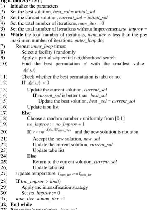
The details of this procedure are summarized in Figure 2. If there is no improvement of the solution obtained within a certain number of iterations (limit), we apply an intensification strategy of Tabu Search. This strategy focuses the search once again starting from the best permutation obtained. Finally, the entire algorithm will be terminated if the total number of iterations of the outer loop reaches the preset maximum number of iterations, outer_loop.

Algorithm SA-TS ( )

(1) Initialize the parameters

(2) Set the best solution, best_sol = initial_sol

(3) Set the current solution, current_sol = initial_sol

(4) Set the total number of iterations, num_iter = 0

(5) Set the total number of iterations without improvement,no_improv = 0

(6) While the total number of iterations, num_iter is less than the preset

maximum number of iterations, outer_loop do:

(7) Repeat inner_loop times:

(8) Select a facility i randomly

(9) Apply a partial sequential neighborhood search

(10) Find the best permutation   _{with the smallest value of}

π,i,j

Δ 

(11) Check whether the best permutation is tabu or not

(12) If Δπ,i,j < 0

(13) Update the current solution, current_sol

(14) If current_sol is better than best_sol

(15) Update the best solution, best _sol = current_sol

(16) Update tabu list

(17) Else

(18) Choose a random number r uniformly from [0,1]

(19) no_improv := no_improv + 1

(20) If rexpΔπ,i,j/Tnum_iter and the new solution is not tabu

(21) Accept the new solution, new_sol

(22) Update the current solution, current_sol

(23) Update tabu list

(24) Else

(25) Return to the current solution, current_sol

(26) Update tabu list

(27) Update temperature Tnum_iter:αTnum_iter

(28) If (no_improv > limit)

(29) Apply the intensification strategy

(30) Set no_improv := 0

(31) num_iter := num_iter +1

(32) End while

(33) Report the best solution, best_sol

Fig. 2 Algorithm SA-TS

IV.COMPUTATIONAL RESULTS

A. Experimental Setup

The values of the parameters used in the computational experiments are determined experimentally to ensure a compromise between the computation time and the solution quality. They are summarized in Table I. The algorithms were implemented using C++ and executed on a 2.67 GHz Intel Core 2 Duo CPU with 3 GB of RAM under the Microsoft Windows Vista Operating System.

TABLE I PARAMETER SETTINGS

Parameter Value

Maximum number of iterations, outer_loop 300n

Initial temperature, T0 5,000

Number of neighborhood moves at each

temperature T, inner_loop 100n

Cooling factor, α 0.9

Number of non-improvement iterations prior to

intensification, Limit 0.02outer_loop

Length of tabu list, length n/2

B. Results

In order to evaluate the performance of our proposed algorithm, we decided to solve some benchmark problems from a library for research on the QAP (QAPLIB) which have been studied and solved by other researchers [31]. For each benchmark problem, the proposed algorithm was executed 20 times with different random seeds.

According to [37], the instances of QAPLIB can be classified into four classes: unstructured (randomly generated) instances, grid-based distance matrix and real-life instances and real-life-like instances. Due to the limitation of the target algorithm that can only solve symmetric instances with zero diagonal values, we only focus on some instances from three classes: unstructured (randomly generated) instances, grid-based distance matrix and real-life instances. Table II presents the instances selected from each class.

TABLE II

PROBLEM INSTANCES

Class Instances

I unstructured (randomly generated) instances had, rou, tai

II grid-based distance matrix nug, scr, sko

II real-life instances chr, kra

The following tables summarize the average objective function value obtained and the best objective function value obtained for each class. The objective function values of the optimal/best known solutions given in Burkard et al. [31] are

also presented for comparison purposes. The heading Φ1

refers to the percentage deviation between the average objective function value of the solutions obtained and the

best known/optimal solution, while the heading Φ2 refers to

the percentage deviation between the best objective function value of the solutions obtained and the best known/optimal

solution. The values for Φ1 and Φ2 are computed as follows:

    

 

 

 

so l ma l kn o wn /o p ti b est

a lg o rith m o f va lu e fu n ctio n o b jective a vera g e so l ma l kn o wn /o p ti b est

1 0 0

Φ₁ (8)

    

 

 

 

so l ma l kn o wn /o p ti b est

a lg o rith m o f va lu e fu n ctio n o b jective b est so l ma l kn o wn /o p ti b est

1 0 0

Φ2 (9)

notice that the average gaps of the solutions are less than or equal to 0.40%. For each problem instance, the hybrid algorithm is again able to obtain the best known/optimal

solutions. The value of Φ1 is not more than 0.03% for rou

problem instances (Table IV).

As shown in Table V, for the tai type benchmarks, the

performance of the proposed algorithm is still acceptable

with values of Φ1 and Φ2 are not more than 3.72% and

3.58%, respectively. For larger problem instances (with n > 20), the best known/optimal solutions cannot be found. It is likely that with greater number of iterations, the outcome may improve with possibility of obtaining the best known/optimal solutions for some of instances.

TABLE III

COMPUTATIONAL RESULTS FOR had PROBLEM INSTANCES

Benchmark problem

Optimal/Best known solution

Average Solution

Best Solution

Φ1

(%)

Φ2

(%)

had12 1652 1652 1652 0.00 0.00

had14 2724 2735 2724 0.40 0.00

had16 3720 3721 3720 0.03 0.00

had18 5358 5358 5358 0.00 0.00

had20 6922 6927.2 6922 0.08 0.00

TABLE IV

COMPUTATIONAL RESULTS FOR rou PROBLEM INSTANCES

Benchmark problem

Optimal/Best known solution

Average Solution

Best Solution

Φ1

(%)

Φ2

(%)

rou12 235528 235528 235528 0.00 0.00

rou15 354210 354210 354210 0.00 0.00

rou20 725522 725742.7 725522 0.03 0.00

TABLE V

COMPUTATIONAL RESULTS FOR tai PROBLEM INSTANCES

Benchmark problem

Optimal/Best known solution

Average Solution

Best Solution

Φ1

(%)

Φ2

(%)

tai10a 135028 135028 135028 0.00 0.00

tai12a 224416 224416 224416 0.00 0.00

tai15a 388214 388214 388214 0.00 0.00

tai17a 491812 491812 491812 0.00 0.00

tai20a 703482 704610.2 703482 0.16 0.00

tai25a 1167256 1182462.3 1175490 1.30 0.71

tai30a 1818146 1845611.7 1833020 1.51 0.82

tai35a 2422002 2484348.1 2477054 2.57 2.27

tai40a 3139370 3228315.1 3207852 2.83 2.18

tai50a 4938796 5122386.6 5115612 3.72 3.58

tai60a 7205962 7463484.2 7417240 3.57 2.93

tai80a 13515450 13997867.4 13938662 3.57 3.13

tai100a 21054656 21788679.9 21689698 3.49 3.02

The computational results for the second class (grid-based distance matrix) are summarized in Tables VI, VII and VIII.

Table VI is a summary of the results for the nug problem

instances. The results indicate that these problem instances do not pose much difficulty for the proposed hybrid

algorithm to obtain good solutions as the values of Φ1 are

not more than 0.02%. All the best known/optimal solutions can be obtained within reasonable computation time, with

the optimal solution to the largest problem instance, nug30,

being obtained within 15 minutes.

Tables VII and VIII show the results of testing on scr and

sko problem instances. The values of Φ1 are 0% for scr

problem instances, while the maximum value of Φ1 is only

0.18% for sko problem instances. For sko49 and sko56, the

values of Φ2 are about 0.1% from the optimal/best known

solution. The longest CPU time required to obtain the solution is about 3 hours for sko56.

TABLE VI

COMPUTATIONAL RESULTS FOR nug PROBLEM INSTANCES

Benchmark problem

Optimal/Best known solution

Average Solution

Best Solution

Φ1

(%)

Φ2

(%)

nug12 578 578 578 0.00 0.00

nug14 1014 1014 1014 0.00 0.00

nug15 1150 1150 1150 0.00 0.00

nug20 2570 2570 2570 0.00 0.00

nug21 2438 2438 2438 0.00 0.00

nug22 3596 3596 3596 0.00 0.00

nug24 3488 3488 3488 0.00 0.00

nug25 3744 3744 3744 0.00 0.00

nug27 5234 5234 5234 0.00 0.00

nug28 5166 5166.9 5166 0.02 0.00

nug30 6124 6124.4 6124 0.01 0.00

TABLE VII

COMPUTATIONAL RESULTS FOR scr PROBLEM INSTANCES

Benchmark problem

Optimal/Best known solution

Average Solution

Best Solution

Φ1

(%)

Φ2

(%)

scr12 31410 31410 31410 0.00 0.00

scr15 51140 51140 51140 0.00 0.00

scr20 110030 110030 110030 0.00 0.00

TABLE VIII

COMPUTATIONAL RESULTS FOR sko PROBLEM INSTANCES

Benchmark problem

Optimal/Best known solution

Average Solution

Best Solution

Φ1

(%)

Φ2

(%)

sko42 15812 15833.8 15812 0.14 0.00

sko49 23386 23424.5 23410 0.16 0.10

sko56 34458 34520.4 34494 0.18 0.10

TABLE IX

COMPUTATIONAL RESULTS FOR chr PROBLEM INSTANCES

Benchmark problem

Optimal/Best known solution

Average Solution

Best Solution

Φ1

(%)

Φ2

(%)

chr12a 9552 9552 9552 0.00 0.00

chr12b 9742 9742 9742 0.00 0.00

chr12c 11156 11156 11156 0.00 0.00

chr15a 9896 9896 9896 0.00 0.00

chr15b 7990 7990 7990 0.00 0.00

chr15c 9504 9504 9504 0.00 0.00

chr18a 11098 11098 11098 0.00 0.00

chr18b 1534 1534 1534 0.00 0.00

chr20a 2192 2224.9 2192 1.50 0.00

chr20b 2298 2306.7 2298 0.38 0.00

chr20c 14142 14142 14142 0.00 0.00

chr22a 6156 6181.3 6156 0.41 0.00

chr22b 6194 6265.2 6194 1.15 0.00

chr25a 3796 3811 3796 0.40 0.00

TABLE X

COMPUTATIONAL RESULTS FOR kra PROBLEM INSTANCES

Benchmark problem

Optimal/Best known solution

Average Solution

Best Solution

Φ1

(%)

Φ2

(%)

kra30a 88900 89554.5 88900 0.74 0.00

kra30b 91420 91420 91420 0.00 0.00

kra32 88700 88700 88700 0.00 0.00

Finally, Table IX and X summarize the results of testing on the third class (real-life instances). Table IX summarizes

difficulty level in solving the chr problem instances is considered significant [25]. On the whole, the proposed

hybrid algorithm is able to find solutions with values of Φ1

not exceeding 1.50% from the known optimum. For all problem instances, the best known/optimal solutions are also obtained.

Tables X summarizes the results of testing on kra problem instances. The average gaps of the solutions are less than 0.75%. For each problem instance, the hybrid algorithm is again able to obtain the best known/optimal solutions.

In summary, we observe that the proposed hybrid algorithm is able to obtain very good or optimal solutions to benchmark problem instances drawn from the QAPLIB. The computation time required to do so is also reasonable especially for problem instances with modest size.

V. CONCLUSIONS

In this paper, a hybrid algorithm that combines GRASP, Simulated Annealing and Tabu Search is proposed to solve the QAP. The proposed algorithm for solving the QAP is able to obtain the optimal or best known solutions for problem instances drawn from the QAPLIB.

There are several issues for future research. First, in the proposed hybrid algorithm, the Tabu Search framework has been designed primarily with short term memory. As part of future research work, the possibility of implementing other Tabu Search strategies, such as long term memory and diversification strategy, within the hybrid algorithm will be considered. Second, different types of hybridization with other metaheuristics, such as the genetic algorithm and ant colony optimization algorithm, can also be investigated. Third, the application of the proposed hybrid algorithm to solve other optimization problems is another area of future research, such as Quadratic Semi Assignment Problem (QSAP).

REFERENCES

[1] E. M. Loiola, N. M. M. de Abreu, P. O. Boaventura-Netto, P. Hahn, and T. Querido, “A survey for the quadratic assignment problem,” European Journal of Operational Research, vol. 176, pp. 657-690, 2007.

[2] T. C. Koopmans, and M. J. Beckmann, “Assignment

problems and the location of economic activities,” Econometrica, vol. 25, pp. 25: 53-76, 1957.

[3] S. Sahni, and T. Gonzales, “P-Complete approximation problems,” Journal of the Association for Computing Machinery, vol. 23, pp. 555-565, 1976.

[4] K. M. Anstreicher, “Recent advances in the solution of quadratic assignment problems,” Mathematical Programming, vol. 97(1-2), pp. 27-42, 2003.

[5] Z. Drezner, P. M. Hahn, and E. D. Taillard, “Recent advances for the QAP problem with special emphasis on instances that are difficult for metaheuristic methods,” Annals of Operations Research, vol. 139, pp. 65-94, 2005.

[6] L. Steinberg, “The backboard wiring problem: a placement algorithm,” SIAM Review, vol. 3, pp. 37-50, 1961.

[7] J. W. Dickey, and J. W. Hopkins, “Campus building arrangement using Topaz,” Transportation Research, vol. 6, pp. 59-68, 1972.

[8] A. N. Elshafei, “Hospital layout as a quadratic assignment problem,” Operations Research Quarterly, vol. 28(1), pp. 167-179, 1977.

[9] A. M. Geoffrion, and G. W. Graves, “Scheduling parallel production lines with changeover costs: practical applications of a quadratic assignment/LP approach,” Operations Research, vol. 24, pp. 595-610, 1976.

[10] L. S. Pitsoulis, P. M. Pardalos, and D. W. Hearn, “Approximate solutions to the turbine balancing problem,” European Journal of Operational Research, vol. 130, pp. 147-155, 2001.

[11] C. A. Fedjki, and S. O. Duffuaa, “An extreme point algorithm for a local minimum solution to the quadratic assignment problem,” European Journal of Operational Research, vol. 156(3), pp. 566-578, 2004.

[12] D. F. Rossin, M. C. Springer, and B. D. Klein, “New complexity measures for the facility layout problem: an empirical study using traditional and neural network analysis,” Computers and Industrial Engineering, vol. 36(3), pp. 585-602, 1999.

[13] M. R. Wilhelm, and T. L. Ward, “Solving quadratic

assignment problem by simulated annealing,” IIE

Transactions, vol. 19(1), pp. 107-119, 1987.

[14] A. M. Frieze, and J. Yadegar, “On the quadratic assignment problem,” Discrete Applied Mathematics, vol. 5, pp. 89-98, 1983.

[15] E. L. Lawler EL, “The quadratic assignment problem,” Management Science, vol. 9, pp. 586-599, 1963.

[16] K. M. Anstreicher, and N. W. Brixius, “A new bound for the quadratic assignment problem based on convex quadratic programming,” Mathematical Programming, vol. 89(3), pp/ 341-357, 2001.

[17] C.S. Edwards, “A branch and bound algorithm for the

Koopmans-Beckmann quadratic assignment problem,”

Mathematical Programming Study, vol. 13, pp.35-52, 1980. [18] D. J. White, “Some concave-convex representations of the

quadratic assignment problem,” European Journal of the Operational Research, vol. 80(2), pp. 418-424, 1995. [19] S. Yamada, “A new formulation of the quadratic assignment

problem on r-dimensional grid,” IEEE Transactions on Circuits and Systems I-Fundamental Theory and Applications, vol. 39(10), pp. 791-797, 1992.

[20] M. H. Lim, Y. Yuan, and S. Omatu, “Efficient genetic algorithms using simple genes exchange local search policy for the quadratic assignment problem,” Computational Optimization and Applications, vol. 15, pp. 249 – 268, 2000. [21] E. D. Taillard, “Robust taboo search for the quadratic assignment problem,” Parallel Computing, vol. 17, pp. 443-455, 1991.

[22] V. Maniezzo, and A. Colorni, “Algodesk: An experimental comparison of eight evolutionary heuristics applied to the quadratic assignment problem,” European Journal of Operational Research, vol. 81(1), pp. 188-204, 1995.

[23] V. Maniezzo, and A. Colorni, “The ant system applied to the quadratic assignment problem,” IEEE Transactions on Knowledge and Data Engineering, vol. 11(5), pp. 769-778, 1999.

[24] R. K. Ahuja, J. B. Orlin, and A. Tiwari, “A greedy genetic algorithm for the quadratic assignment problem,” Computers and Operations Research, vol. 27, pp. 917-934, 2000. [25] M. H. Lim, Y. Yuan, and S. Omatu, “Extensive testing of a

hybrid genetic algorithm for solving quadratic assignment problems,” Computational Optimization and Applications, vol. 23, pp. 47-64, 2002.

[26] Z. Drezner, “The extended concentric tabu for the quadratic assignment problem,” European Journal of Operational Research, vol. 160, pp. 416-422, 2005.

[28] P. Tian, H. C. Wang, and D. M. Zhang, ”Simulated annealing for the quadratic assignment problem: a further study,” Computers and Industrial Engineering, vol. 31(3-4), pp. 925-928, 1996.

[29] A. Misevicius, “An improved hybrid optimization algorithm for the quadratic assignment problem,” Mathematical Modelling and Analysis, vol. 9(2), pp. 149-168, 2004. [30] H. Youssef, S. M. Sait, and H. Ali, “Fuzzy simulated

evolution algorithm for VLSI cell placement,” Computers and Industrial Engineering, vol. 44(2), pp. 227-247, 2003. [31] R. E. Burkard, S. E. Karisch, and F. Rendl, “QAPLIB – a

quadratic assignment problem library,” Journal of Global Optimization, vol. 10, pp. 391-403, 1997.

[32] L. Yong, P. M. Pardalos, and M. G. C. Resende, “A greedy randomized adaptive search procedure for the quadratic assignment problem,” in P. M. Pardalos, and H. Wolkowicz (Eds.), Quadratic assignment and related problems: DIMACS Workshop. DIMACS Series in Discrete Mathematics and Theoretical Computer Science, vol. 16, pp.237-261, 1994.

[33] S. Kirkpatrick, C. D. Gellatt, and M. P. Vecchi, “Optimization by simulated annealing,” Science, vol. 220, pp. 671-680, 1983.

[34] F. Glover, “Tabu search – part I,” ORSA Journal on Computing, vol. 1, pp. 190-206, 1989.

[35] F. Glover, “Tabu search – part II,” ORSA Journal on Computing,” vol. 2, pp. 4-32, 1990.

[36] É. D. Taillard, and L. M. Gambardella, “Adaptive memories for the quadratic assignment problem,” Technical Report IDSIA-87-97, IDSIA, Lugano, Switzerland, 1997.

[37] É. D. Taillard, “Comparison of iterative searches for the