A Modified Multi Time Step Integration for Dynamic Analysis

A Modified Multi Time Step Integration for Dynamic Analysis

J. Alamatian*

Civil Engineering Department, Mashhad Branch, Islamic Azad University, Mashhad, Iran, 91735-413

P A P E R I N F O

Paper history:

Received 7 June 2012

Received in revised form 18 July 2012 Accepted 30 August 2012

Keywords: Dynamic Analysis Implicit Multi Time Step Higher Order Integration

A B S T R A C T

This paper deals with new implicit multi time step integration for numerical dynamic analysis in constant time step. The proposed method tries to improve the main difficulties of the multi time step integrations i.e. high calculations and also high required memory. For this purpose, several previous velocity and acceleration vectors are used to integrate the displacement and velocity of the current time step, respectively. It could be shown that only one set of weighted factors appears in the proposed technique so that the computational efforts and the required memory reduce compared with the similar multi time step integrations which use several groups of weighted factors for controlling the stability and the accuracy. Therefore, simplicity, lower computational tasks and lower required memory are the main advantages of the new integration which made this method suitable for nonlinear dynamic analysis of large systems. Here, the Taylor series expansion and the Routh-Hurwitz criterion are utilized to calculate the weighted factors and determine the stability domain of the proposed integration, respectively. For numerical verification, some dynamic systems i.e. the nonlinear vibration, the portal frame and the elastic pendulum are analyzed to clarify the ability and the efficiency of the new method. Results show that by a similar time step, the proposed time integration is more accurate and more rapid compared with the common approaches such as the Wilson-θ, the Newmark-β and some other multi time step schemes.

doi: 10.5829/idosi.ije.2012.25.04b.06

NOMENCLATURE

[ ]n1

C + Damping matrix in n+1th time step

[ ]

Zm´m Coefficient matrix for integration’s order m

{ }n1

D + Displacement vector in n+1th time step Greek Symbols

{ }

n 1

D& + Velocity vector in n+1th time step ξ Displacement weighted factor for IHOA

{ }

n 1

D&& + Acceleration vector in n+1th _{time step η Velocity weighted factor for IHOA}

{ }D0 Initial displacement vector a Displacement weighted factor for N-IHOA

{ }D&0 Initial velocity vector g Velocity weighted factor for N-IHOA

{ }

n 1 Exact

D + Exact displacement vector in n+1th time step Δt Time step

{ }

n 1 Exact

D& + Exact velocity vector in n+1th _{time step}

cr

Δt Critical time step

{ }

n 1

f + Internal force vector in n+1th time step λ Eigenvalue

[ ]n 1

M + Mass matrix in n+1th time step Ω Circular frequency

{ }

n 1 EQ

P + Equivalent external force vector in n+1th time step w Natural frequency

* Corresponding Author Email: alamatian@yahoo.com (J. Alamatian)

{ }

n 1 D

R + Displacement residual vector in n+1th _{time step}

Superscripts

{ }

n 1

V

R + Velocity residual vector in n+1th _{time step n Time step}

[ ]n 1

EQ

S + Equivalent stiffness matrix in n+1th time step m Integration’s order

1. INTRODUCTION

Numerical methods which are widely used in dynamic analyses try to obtain the answer of a second order time differential equation with some initial conditions as follows:

{

} {

}

n 1 _{n 1} n 1

n 1 _{n 1 n 1}

M + ì üD + é ùC + ìDü + f(D +) P(t +)

é ù _{í ý í ý}

ë û _î&&_þ +ë û _î&_þ + =

{ }

D(0) =

{ }

D0 ,

{ } { }

D&(0) = D&0

(1)

Here,

[ ]

n1

M + ,

[ ]

Cn+1,

{

f(Dn+1)

}

and

{

P(tn+1)

}

are mass matrix, damping matrix, internal and external forces vectors, respectively. In addition,

{ }

n1

D + is the nodal displacement vector and super dots denotes differential with respect to the time. All of these quantities are calculated at timetn+1, called the current time step. Here,

{ }

D₀ and

{ }

D&₀ are displacement and velocity vectors at t=0, respectively. Numerical schemes are classified in three general groups: Implicit, Explicit and predictor-corrector. In each step of implicit methods, the dynamic equation is transformed to the equivalent static system. High accuracy and more stable analysis are the main advantages of the implicit integrations especially in nonlinear dynamics. However, the cost and the computational time may dramatically increase for large scale structures with huge number of degrees of freedom. The Newmark-β method, Wilson-θ procedure, generalized-α method [1], HHT-α [2], WBZ-α [3], the Newmark multi time step approach [4], the third order time step integration [5], the Newmark complex time step [6], the time weighted function procedure [7], the generalized single step integration [8], the Nørsett time integration [9], the composite time integration [10], the higher order acceleration function [11], the implicit integration based on the conserving energy and momentum [12], the Green function approach [13, 14], the precise integration methods [15], the implicit higher order time integration [16] and the backward Euler time-integration method [17] are some well known implicit integrations.

In the explicit methods, displacement and velocity of the current time step are calculated by only vector operations based on the previous time step data. Then, the acceleration vector will be obtained by solving a linear system of equations formulated from the dynamic equation of motion [18-21]. These methods are quite

simple; however there are serious concerns about their accuracy and stability.

Combining the implicit and the explicit techniques leads to an interesting approach called predictor-corrector algorithms. In such methods, the explicit procedures are used to obtain an estimation of the answer. This estimation is corrected by the implicit relationships. As a result, calculations are in vector form and because of using implicit equations; the numerical instability will be limited [22, 23]. These specifications cause that the predictor-corrector methods are utilized for different analyses such as structural control [24].

In this paper, a new multi-time step integration which belongs to the implicit methods is presented for dynamic analysis. Here, the current displacement and velocity vectors are proposed to be functions of the velocity and acceleration vectors of several previous time steps, respectively. The unknown parameters are calculated in the manner that the suggested time integration has maximum accuracy. Moreover, studying the stability conditions of this integration leads to the acceptable zone for choosing time step. To verify the numerical ability of the proposed method, some dynamic systems are analyzed.

2. NEW IMPLICIT HIGHER ORDER ACCURACY

(N-IHOA)TIMEINTEGRATION

{ }

n 1

{ }

n n m -1 ₂ n i

i 0 n 1 m -1 n i

2 2

0 i

i 1 1

D D Δt D (₂ ξ) Δt D

ξ Δt D Δt ξ D

+ ì ü ì ü

í ý í ý

î þ ₌ î þ

+

-ì ü ì ü

í ý í ý

î þ ₌ î þ

= + + - å

+ + å

& &&

&& &&

₍₂₎

n 1 n m - 1 n n 1

0 i

i 0 m - 1 n i

i i 1

D D (1 η) Δt D η Δt D

Δt η D

+ +

ì ü ì ü ì ü ì ü

í ý í ý í ý í ý

î þ î þ î þ î þ

= -ì ü í ý î þ =

= + - å +

+ å

& & && &&

&& (3)

where,

{ }

D&& n-i is the acceleration vector at n-i th _time station. This quantity is available from the previous steps. Furthermore, ξ_i and η_i are weighted factors which control the stability and accuracy of time integration. These factors have been calculated for maximum accuracy [16]. In addition, time step (Δt) has been limited by the stability domain of the integration [16].

For purposing a new version of the IHOA method, the displacement and velocity vectors of the current time step are assumed to be functions of the velocities and accelerations of several previous steps, respectively, as follows:

{ }

{ }

{ }

{ }

n

m 1 _{n 1}

n 1 n

D i

i 1 m 1 n i

i i 1

D

D D Δt(1 ) D Δt

Δt

a a a

a

+

+ ì ü

í ý î þ = -= -¢ ¢

= + - - å + +

å & & & (4)

{ }

{ }

{ }

n 1 n m _{n n 1}

D D

i i 1

m n i

i i 1

1

1 D

D D Δt(1 ) Δt

Δt

g g g

g

+ ₊

ì ü ì ü

í ý í ý

î þ î þ

= -= -¢ ¢

= + - - å + +

å

&& &&

&& & &

(5)

Here, a and g are weighted factors of new integration. Equations (4) and (5) present the fundamental equations of the proposed time integration which uses the velocities and accelerations of several previous time steps. To formulate the solution algorithm of the new method, the current velocity vector i.e.

{ }

n1

D& + is obtained from Equation (4):

{ }

{ }

{ }

{ }

n 1

m 1 _n m 1 _{n i} (1 _i) D Δt _i D

i 1 i 1

D

n 1 n

D D

Δt

a a a

a a + ì ü í ý î þ - - -¢

- - å + å

= = = ¢ + -¢ & & & (6)

By substituting Equation (6) in Equation (5), the current acceleration vector i.e.

{ }

D&& n+1obtains;

{ }

{ }

{ }

{ }

{ }

{ }

{ }

n 1 D

m 1 n m 1 n i (1 _i) D _i D

i 1 i 1

Δt

m 1 _{n n 1}

(1 ) D D

n 1 n _i

D D _{i 1}

2 Δt

a a

a g

g g g

g a g

+

- -

-- å + å

= =

=

-¢ -¢

- ₊

¢ ¢

- - å +

+ - ₌ -¢ ¢ ¢ && & &

&& && (7)

Finally, an equivalent static system is achieved if Equations (6) and (7) are substituted into Equation (1),

[ ]

{ }

{ }

n 1

EQ 1 n 1 n

EQ D P

S + + = + (8)

where,

[ ]

n 1 EQ

S + and

{ }

n 1 EQ

P + are the equivalent secant stiffness matrix and the equivalent load vector, respectively. These quantities are formulated as follows,

n 1 n 1 ₀ n 1 n 1

2 EQ

η 1

S M C S

Δt

Δt a

a g

+ + + +

é ù é ù é ù é ù

ë û

ë û = _{¢ ¢} + _¢ ë û +ë û (9)

{ }

{

}

[ ]

{ }

{ }

{ }

[ ]

{ }

{ }

[ ]

{ }

{ }

{ }

_÷÷ ø ö çç è æ ÷÷ ø ö çç è æ ÷÷ ø ö çç è æ å -= -+ å -¢ -+ ¢ + ¢ + å -¢ -¢ + å + å -+ ¢ ¢ + = -= + + -= + -= -= + + + 1 m 1 i i n D i Δt D ) Δt(1 D C Δt 1 D D ) (1 M 1 D Δt D ) Δt(1 D M Δt 1 ) P(t P n 1 m 1 i i n 1 n 1 n n 1 m 1 i i 1 n 1 m 1 i i n i n 1 m 1 i i n 1 n 2 1 n 1 n EQ & & && && & & a a a a g g g g a a g a (10)

The displacement vector of the current time step i.e.

{ }

_D n+1_{is calculated by solving Equation (8) in each time} step. Then, the current velocity and acceleration vectors are obtained from Equations (6) and (7), respectively. This procedure is repeated for the next time step until the analysis time is completed.

It should be noted that the explicit Dynamic Relaxation (DR) method is utilized here for solving Equation (8). As described in the recent papers, the Dynamic Relaxation method which can be successfully combined with the implicit time integrations causes considerable reduction in numerical errors [26]. Simplicity, vector operators and higher efficiency in nonlinear systems are the other advantages of DR method. Therefore, Dynamic Relaxation method is employed here to solve the system of simultaneous equations i.e. Equation (8).

m=2. At this stage, three dynamic equilibrium points i.e. n, n-1 and n-2 exist so that the next increment could be started by m=3. This procedure is repeated until the accuracy order of the integration reaches to the selected value.

3. ACCURACY AND STABILITY

In the previous section, a new time integration called N-IHOA has been formulated for dynamic analysis. There are some weighted factors in the proposed relationships which should be determined. If the integration’s order be m, there are 2×m un-known parameters in the N-IHOA relationships. These parameters are calculated so that the numerical accuracy is maximized. It should be emphasized that the stability condition is verified by limiting the time step size.

In numerical methods, there are two sources of error, generally, i.e. the integration’s error and the

numerical error. The numerical errors belong to the

computer’s calculations which the values are not saved exactly. Because of high number of calculations, these errors may increase in dynamic analyses. Using double precision variables, these errors could be limited as performed here. On the other hand, the integration’s errors happen because of non continuity of higher order displacement’s derivatives such as third order, forth order, fifth order and etc. The reason for this subject could be explained as follows. The dynamic equation of motion is a second order time differential relationship which only uses the first and the second order derivatives of the displacement. In the other words, higher order derivatives such as third order, forth order and etc do not appear directly in the dynamic equation of motion. The non continuity of higher order derivatives between successive time steps causes the integration’s error. The proposed method tries to improve this defect by applying the continuity conditions for more number of higher order displacement’s derivatives.

For calculating the weighted factors, the error functions of the current displacement and velocity vectors could be defined as follows:

{ }

n 1

{ }

n 1

{ }

n 1

Exact

D D

R + = D + - + (11)

{ }

{ }

{ }

n 1

Exact 1

n 1

n _{D D}

V

R + = & + - & + (12)

where,

{ }

n1

D

R + and

{ }

R nV1

+ _{are the current residual vectors}

of the displacement and velocity, respectively. The exact displacement and velocity vectors, i.e.

{ }

n 1

Exact

D +

and

{ }

n1 Exact

D& + are obtained from the Taylor series expansion:

{ }

{ }

{ }

{ }

{ }

{ }

n n n

n _{2 3 3}

n 4 4

n 1

D Δt D Δt D 0.1667Δt D Exact

0.0417Δt D

D + 0.5 +

+ +

= + & + &&

K (13)

{ }

{ }

{ }

{ }

{ }

n n _{2 3} n _{3 4} n

n 4 5

n 1

D Δt D 0.5Δt D 0.1667Δt D Exact

0.0417Δt D

D +

ì ü _{+ + +}

í ý î þ

+ +

= & &&

K

&

(14)

here,

{ }

_i n

D is the ith displacement’s derivative order of the nth _{step. Since the exact solution vectors, i.e.} Equations (13) and (14) are functions of the displacement’s derivatives of the nth _{increment, the} current displacement and velocity vectors, i.e. Equations (4) and (5) should also be formulated based on the displacement’s derivatives. For this purpose, the inverse expansions of the velocity and acceleration vectors give [16],

{ }

_{n i} k k _{k 1} n i 1

D

k 0 i 1 , 2...m

( 1) Δt _D k!

- +

- ì + ü

í ý

î þ

= =

¥

-= å

&

(15)

k k

n i _{k 2} n i 1

k 0 i 1, 2...m

( 1) Δt

D D

k!

- _{ì ü} - +

ì ü +

í ý í ý

î þ î þ

= =

¥

-= å

&&

(16)

Similar relationship could be written for the inverse expansion of the jth _{order of the displacement’s} derivative,

{ }

_j n i k k _{j k} n i 1

k 0 i 1 , 2 ...m , j 1 , 2 ...

( 1 ) Δt

D D

k !

- + ¥

- _{ì + ü}

í ý

î þ

=

= = ¥

-= å

(17)

If Equations (15) to (17) are iterated successively, the previous velocity and acceleration vectors are formulated in the terms of the displacement’s derivatives of the nth _{step. For example, the current} displacement and velocity vectors for the first and second accuracy order i.e. m=1 and m=2 are as follows;

{ }

{ }

{ }

{ }3

1

n _n

n 1 n

D n

D

2

D D D ( )

1 3

(0.5 0.5 )

t t

t

a a

a a

+ _{ì ü}

í ý

î þ

¢

¢

= + D + - D +

+ D +

&&

&

K m=2 (18)

{ }

{ }

{ }

{ }

3

4 1

n 1 _{n n}

D D D

n D

2

D ( )

1 3

(0.5 0.5 )

t t

t

g g

g g

+

ì ü

í ý

î þ

¢

¢

= + D + - D +

+ D +

& &&

&

K m=2 (19)

{ } { } { }

{ }

{ }

3 1

4 1

n _n

n 1 n

D

n D

n D

2

D D D ( 2 )

1 2

3

(0.5 0.5 2 )

2

4 (0.1667 0.1667 1.3333 )

2

t t

t

t

a a

a a

a a a

a

a

+ ì_í ü_ý î þ ¢

¢

¢

= + D + - - D

+ + + D +

- - D +

&&

&

K

{ } { } { } { } 3 4 1 5 1

n 1 n _{n n}

D D n D n D 2

D D ( ₁ 2 ₂)

3

(0.5 0.5 2 )

2

4 (0.1667 0.1667 1.3333 )

2

t t

t

t

g g g

g g g

g g g

+ ì ü ì ü í ý í ý

î þ =î þ + D + ¢- - D +

¢ + + D +

¢ - - D +

&&

& &

K

m=3 (21)

By comparing either Equation (18) with Equation (19) or Equation (20) with Equation (21), the most important specification of the N-IHOA is clarified. It means if the integration order is selected as m, the coefficients of the weighted factors in both displacement and velocity vectors are the same. In the other words, the proposed formulation of the N-IHOA method leads to the only one set of independent

weighted factors so that the numerical values of the

weighted factors in the proposed displacement and the velocity vectors (Equations 4 and 5) are the same, i.e.

g

a¢= ¢ and ai =gi i=1,2,...m-1. It should be noted that the IHOA method has two set of independent weighted factors (ξ_i and η_i) which have different values [16]. Consequently, if the integration order be m, the N-IHOA and the IHOA have m and 2×m independent weighted factors, respectively. Therefore, the N-IHOA will be simpler than the IHOA technique; because in the IHOA two set of weighted factors (ξ and

η) should be calculated and saved. Low number of weighted factors in the proposed N-IHOA algorithm leads to reduction in required memory for the dynamic analysis and its programming will be simpler than the IHOA. In addition, it is expected that the analysis time of the N-IHOA may be less than the IHOA. This subject will be verified numerically. Such specifications cause that the proposed method has a potential which makes it suitable for using in the commercial structural analysis software.

On the other hand, the maximum accuracy will occur if the maximum possible number of the coefficients in the displacement and the velocity residual vectors i.e.

{ }

n1

D

R + and

{ }

R nV1

+ _{are zero. To}

explain this procedure, let the accuracy order be 3 (m=3). Substituting Equations (13) and (20) into (11) and Equations (14) and 21 into (12) gives:

{ } { } { } { } D 3 1 1 4 n n 1 R D n D n D 2

( 2 0.5)

1 2

3

(0.5 0.5 2 0.1667)

2

(0.1667 0.1667 1.3333 0.0417) 2 4 t t t a a a a

a a a

a a + ¢ ¢ ¢

= - - - D

+ + + - D +

- - -D + && L m=3 (22) { } { } { } { } 3 V 4 1 5 1 n n 1 R D n D n D 2

( 2 0.5)

1 2

3 (0.5 0.5 2 0.1667)

2

4 (0.1667 0.1667 1.3333 0.0417)

2

t t

t

g g g

g g g

g g g

+ _{= ¢- - - D +}

¢ + + - D +

¢ - - - D +L

m=3 (23)

The right hand sentences of Equations (22) and (23) have the same coefficients which confirm the dependency of weighted factors in the N-IHOA method i.e. a¢=g¢, a₁=g₁ and a₂ =g₂. From this point of view, Equations (22) and (23) are similar. Since there are three weighted factors in each residual vector, the maximum numerical accuracy is achieved when the coefficients of three first sentences in Equation (22) or (23) are equal to zero;

1 2

1 1 2 0.5

0.5 0.5 2 0.1667

0.1667 0.1667 1.3333 0.0417 a

a a ¢

ì ü ì ü

-

-é ù

ï ï ï ï

ê ú_{í ý í ý}

ê ú

ï ï ï ï

ê - - ú

ë û î þ î þ

= m=3 (24)

1 2

1 1 2 0.5

0.5 0.5 2 0.1667

0.1667 0.1667 1.3333 0.0417

b b b

¢

ì ü ì ü

-

-é ù

ï ï ï ï

ê ú

í ý í ý

ê ú

ï ï ï ï

ê - - ú

ë û î þ î þ

= m=3 (25)

As expected, the system of Equations (24) and (25) are the same. Generally, this procedure leads to the following linear systems of equations, if the accuracy order be m;

[ ] [ ] ï ï ï ï ï þ ïï ï ï ï ý ü ï ï ï ï ï î ïï ï ï ï í ì ï ï ï þ ïï ï ý ü ï ï ï î ïï ï í ì ¢ ï ï ï ï ï þ ïï ï ï ï ý ü ï ï ï ï ï î ïï ï ï ï í ì ï ï ï þ ïï ï ý ü ï ï ï î ïï ï í ì ¢ + = + = -´ ´ 1)! (m 1 . . . 3! 1 2! 1 . . . Z 1)! (m 1 . . . 3! 1 2! 1 . . . Z 1 m 1 1 m 1 m m m m b b b a a a and (26)

Here,

[ ]

Z_m´_m is a m×m constant matrix. For example,

this matrix has been calculated for some integration’s order (m=1, 2, 3, 4and 5) as follows;

[Z]1×1=[ ]1, [Z]2×2=

úû ù êë é -5 . 0 5 . 0 1 1 _,

[Z]3×3=

ú ú û ù ê ê ë é -3333 . 1 1667 . 0 1667 . 0 2 5 . 0 5 . 0 2 1 1 ,

[Z]4×4=

ú ú ú û ù ê ê ê ë é -375 . 3 6667 . 0 0417 . 0 0417 . 0 5 . 4 3333 . 1 1667 . 0 1667 . 0 5 . 4 2 5 . 0 5 . 0 3 2 1 1 ,

[Z]5×5=

ú ú ú ú û ù ê ê ê ê ë é -5333 . 8 025 . 2 2667 . 0083 . 0083 . 6667 . 10 375 . 3 6667 . 0 0417 . 0 0417 . 0 6667 . 10 5 . 4 3333 . 1 1667 . 0 1667 . 0 8 5 . 4 2 5 . 0 5 . 0 4 3 2 1 1 (27)

and velocity by an accuracy order _Δtm+2_{, respectively.} In the linear Newmark-β, central finite difference and Zhai method, accuracy order related to displacement and velocity are _Δt3 _{and Δt}2_{, respectively. The least} integration’s order of the N-IHOA technique is 1. If the integration’s order is at least (m=1), the accuracy order of both displacement and velocity will be _Δt3_{. For} higher order of the proposed integration, the accuracy order of both displacement and velocity are higher than the well-known existing methods such as linear Newmark-β and central finite difference schemes. Moreover, comparing the IHOA and N-IHOA show that for the same integration’s order, the displacement’s accuracy of the IHOA and N-IHOA algorithms is _Δtm+3 and _Δtm+2_{, respectively. From the mathematical point} of view, the displacement’s accuracy of the IHOA is one order higher than the N-IHOA. However, both methods present the velocity by the same accuracy order i.e. _Δtm+2_.

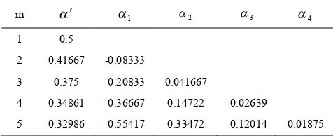
On the other hand, the numerical weighted factors, presented here, are unique and they are not dependent on the problem’s specification. These linear systems have been solved for some accuracy order i.e. m=1,2…5, and the numerical values of weighted factors have been inserted in Table 1.

TABLE 1. Optimum values of weighted factors for the N-IHOA

m a¢ a₁ a2 a3 a4

1 0.5

2 0.41667 -0.08333

3 0.375 -0.20833 0.041667

4 0.34861 -0.36667 0.14722 -0.02639

5 0.32986 -0.55417 0.33472 -0.12014 0.01875

On the other hand, the time step size of dynamic analysis is determined so that the stability conditions are satisfied. This study is performed for an undamped single degree-of-freedom system in free vibration [19];

m s ω , 0 D ω

D&& + 2 = = (28)

where,

w

is the natural frequency. Determining the acceptable time step size is the most common strategy for verifying the numerical stability of the proposed integration. Whatever the acceptable time step domain is larger, the method will be more stable. For this purpose, the weighted factors which calculated previously are used. From Table 1, the numerical values of these parameters are replaced in Equations (4) and (5). First, the fundamental relationship of the N-IHOA should be written in the differential form. The

differential form is a shape that the fundamental relationships i.e. Equations (4) and (5) are only formulated based on the displacement of several successive steps. These formulations are similar to those performed for the IHOA [16]. For example, differential form of the N-IHOA method for the integration’s order 1, 2 and 3 will be as follows;

2 n 2 2 n 1

2 n

(0 .5 0 .1 2 5Ω )D (0 .1 2 5Ω 1)D 0 .5Ω D 0

+ +

+ +

-+ = m=1 (29)

2 n 5 2 n 4

2 n 3 2 n 2

2 n 1 2 n

(0.4167 0.0723Ω )D (0.2364Ω 0.75)D (0.4167 0.2143Ω )D (0.0346Ω 0.0833)D

0.00088ΩD 0.00006ΩD 0

+ +

+ +

+

+ + - +

+ +

-+ - =

m=2 (30)

2 n 8 2 n 7

2 n 6 2 n 5

2 n 4 2 n 3 2 n 2 2 n 1 2 n

(0.375 0.0527Ω )D (0.264Ω 0.5834)D (0.0001 0.2694Ω )D (0.25 0.0675Ω )D (0.0417 0.0467Ω )D 0.0292Ω D 0.0078Ω D 0.001Ω D 0.0417Ω D 0

+ +

+ +

+ +

+ +

+ + - +

+ + -

-+ + +

+ - =

m=3 (31)

where, Ωdefines as below,

ωΔt

Ω= (32)

These differential equations could be transformed to the eigenvalue problems;

2 2 2 2

(0.5 0.125+ Ω )l +(0.125Ω -1)l+0.5Ω =0 m=1 (33)

5 4

3

2 2

2 2 2

2 2

(0.4167 0.0723Ω ) (0.2364Ω 0.75) (0.4167 0.2143Ω ) (0.0346Ω 0.0833) 0.00088Ω 0.00006Ω 0

l l

l l

l

+ + - +

+ + - +

- =

m=2 (34)

8 7

6 5

4 3

2 2

2 2

2 2

2 2 2 2

(0.375 0.0527Ω) (0.264Ω 0.5834) (0.0001 0.2694Ω ) (0.25 0.0675Ω ) (0.0417 0.0467Ω) 0.0292Ω 0.0078Ω 0.001Ω 0.0417Ω 0

l l

l l

l l

l l

+ + - +

+ + -

-+ + +

+ - =

m=3 (35)

and the method of applying the previous information are completely different between the IHOA and N-IHOA schemes. The proposed N-IHOA method uses both velocities and accelerations of the previous steps simultaneously, however; the IHOA only utilizes the accelerations of the previous increments.

It should be emphasized that the proposed integration has been formulated with constant time step. The variable time step may decrease the accuracy and stability of the N-IHOA. The reason for this subject is that the weighted factors and also the stability domains have been studies under the assumption of constant time step. Therefore, the concept of using the variable time step is an interesting subject in multi time step integrations which is the aim of the future researches.

TABLE 2. Stability condition for different accuracy order of the N-IHOA

Integration’s order (m) Dtcr

IHOA N-IHOA

1 0.5513T 0.5196T

2 0.3899T 0.3052T

3 0.2832T 0.2605T

4 0.2586T 0.2568T

5 0.2564T 0.2407T

6 0.2682T 0.2416T

4. NUMERICAL STUDIES

In two previous sections, the fundamental relationships of the N-IHOA followed with the calculations of the weighted factors and stability conditions have been presented. Here, the N-IHOA algorithm is utilized for numerical analysis of some dynamic systems. For this propose, a computer program, using Fortran Power Station software, has been written by the author. Some bench mark problems which their exact solutions are available are solved to verify the validity of the prepared computer’s program and also the proposed numerical method.

Wide range of dynamic systems such as linear and nonlinear, single and multi degree of freedom, damped and un-damped, free and forced from finite element and finite difference, for different kinds of structures i.e. Euler beam and portal frame are used to verify the proposed N-IHOA integration in comparison with some other existing methods. For this purpose, results of the N-IHOA (NI) are compared with some well-known schemes such as Newmark linear acceleration approach (LA), Wilson-θ (WT) and trapezoidal method (CA). Moreover, some problems are utilized to compare the ability and efficiency of the proposed method (N-IHOA) with the IHOA scheme.

4. 1. The Nonlinear Free Vibration The nonlinear free vibration of a dynamic system with the following equation of motion and initial values is going to be solved [27],

5 . 0 (0) D 0 D(0)

0 00D 0 1 500D D 100

D 2 3

= =

= +

+ +

& &&

(36)

The quasi-exact solution is obtained using higher order integrations i.e. the Bathe method with small time step 0.0005 sec. Two time steps as 0.033 and 0.025 second are utilized for the numerical dynamic analysis. Figures 1 and 2 show the displacement response of this vibration between times 9 and 10 second. In both time steps, the error of the NI4 and NI5 is less than other methods (Newmark and Wilson-θ) so that these proposed integrations could present the response of nonlinear vibration with less error. In the other words, the error of the NI1, NI2 and NI3 algorithms is more than the NI4 and NI5. By reducing time step in Figures 2, these methods come near to the exact solution. It should be noted that the proposed NI4 and NI5 time integrations have the highest efficiency in this nonlinear vibration.

-0.06 -0.04 -0.02 0 0.02 0.04 0.06

9 9.2 9.4 9.6 9.8 10

Exact WT CA LA NI1

NI2 NI3 NI4 NI5

D

(m)

t (sec)

Figure 1. Response of the nonlinear free vibration for time step 0.033 s

-0.06 -0.04 -0.02 0 0.02 0.04 0.06

9 9.2 9.4 9.6 9.8 10

Exact WT CA LA NI1

NI2 NI3 NI4 NI5

t (s ec)

D

(m)

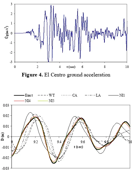
4. 2. Portal Frame Under Based Excitation A concrete plane frame with two bays and three stories (see Figure 3) is analyzed under El Centro based acceleration [28]. This structure has elastic geometrically nonlinear behavior and the co-rotational finite element formulation is used to model this nonlinearity [29]. The cross section and moment of area of beams and columns are 0.40 m2_{, 0.03333 m}4_{, 0.64 m}2 and 0.03413 m4_{, respectively. The mass matrix is} consistent [30] and in order to account for typical additional masses such as slabs, floors, ceilings and etc., material density is assumed to be 1000 times the mass density of concrete i.e. ρ=2500000 kg/m3_.

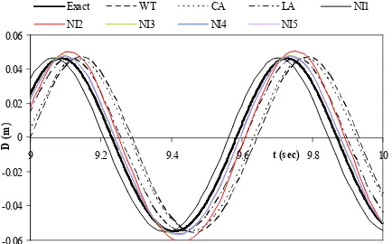
By applying the El Centro ground acceleration (see Figure 4) and using two time steps as 0.02 sec and 0.01 sec, the dynamic response of the structure is calculated within duration of 10 seconds. Figures 5 and 6 show the horizontal response of top of the frame when time step is 0.02 sec and 0.01 sec, respectively. If time step is 0.02 sec, the NI2 and NI3 procedures are unstable; but the NI1, NI4 and NI5 integrations can present the time response curve. Figure 5 also shows that the proposed NI4 and NI5 schemes are more accurate than the well known methods such as Wilson-θ and Newmark-β so that the NI4 and NI5 integrations present the quasi-exact solution which is obtained by the higher order integration i.e. the Bathe method with time step 0.0005 sec. As a result, the NI4 and NI5 methods have an excellent efficiency in the nonlinear dynamic analysis of finite element models. By reducing time step to 0.01 sec, all orders of the proposed method (NI1, 2…7), converge to the exact solution and their accuracy is higher than the common methods (Figure 6).

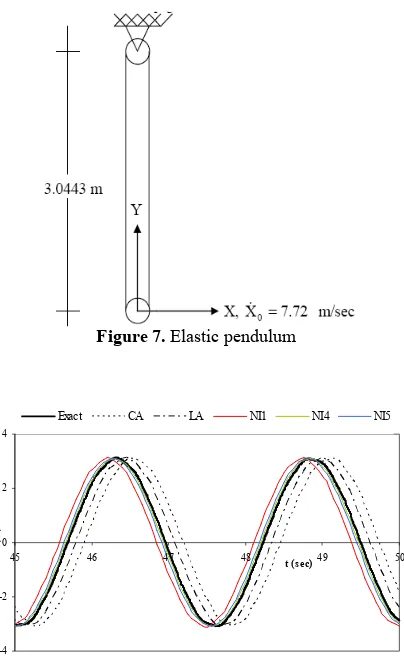
4. 3. Elastic Pendulum Figure 7 shows an elastic pendulum which is modeled by a two nodes truss element [12]. This structure has large deflection nonlinearity. Here, total Lagrange finite element approach is utilized to form the nonlinear equilibrium equations. The mass matrix is consistent [30] and the axial rigidity (AE) and material density per element length (ρA) are 104 _{N and 6.57 kg/m, respectively.} Using two time steps as 0.05 sec and 0.01 sec, Bathe has been analyzed this structure in a small time domain between 0 to 5 seconds. Here, the analysis time domain is extended to 50 seconds and time step is considered as 0.05 sec. Figure 8 shows the response of the horizontal displacement of the pendulum.

The exact solution has been obtained by the Bathe method with small time step 0.0001 sec. By this time step, some methods such as the Wilson-θ, NI2 and NI3 have many fluctuate and they will be unstable. From Figure 8, it is clear that the proposed NI1, NI4 and NI5 producers are more accurate than the Newmark methods so that the NI4 and NI5 integrations present the semi-exact solution.

Figure 3. Portal frame under based excitation

-3 -2 -1 0 1 2 3

0 2 4 t (sec) 6 8 10

Üg

(m

/s

2)

Figure 4. El Centro ground acceleration

-0.03 -0.02 -0.01 0 0.01 0.02 0.03

9 9.2 9.4 9.6 9.8 10

t (s ec)

D

(m)

Exact WT CA LA NI1

NI4 NI5

Figure 5. Response of Horizontal displacement of top of the frame for time step 0.02 s

-0.03 -0.02 -0.01 0 0.01 0.02 0.03

9 9.2 9.4 9.6 9.8 t (sec)10

D

(

m)

Exact WT CA LA NI1 NI2

NI3 NI4 NI5 NI6 NI7

Therefore, the proposed time integration has very good efficiency in nonlinear dynamic analysis. Moreover, this example is utilized to compare the IHOA and NI time integrations. Using time step as 0.05 sec, all accuracy order of the IHOA procedure (IHOA-1, IHOA-2, IHOA-3, IHOA-4 and IHOA-5) present unique response which has been shown in Figure 9.

Figure 7. Elastic pendulum

-4 -2 0 2 4

45 46 47 48 _{t (sec)}49 50

DX

(

m)

Exact CA LA NI1 NI4 NI5

Figure 8. Response of horizontal displacement of the elastic pendulum for time step 0.05 sec

-4 -2 0 2 4

45 46 47 48 t (m)49 50

DX

(

m)

Exact IHOA-1, 2, 3, 4, 5 NI1 NI4 NI5

Figure 9. Response of horizontal displacement of elastic pendulum with IHOA and N-IHOA for time step 0.05 s

From Figure 9 it is concluded that the proposed NI1, NI4 and NI5 procedures have more accuracy than the IHOA integrations. It should be noted that by increasing time step, i. e. 0.075 sec., the proposed time integrations (NI methods) will be unstable, however the IHOA procedures are stable and can present the response by some few errors. Therefore, the IHOA is more stable than the N-IHOA.

4. 4. Euler Beam Here, the vibration of clamped Euler beam is analyzed by the proposed method. The governing equation for the Euler beam’s motion is as follows [4];

) ( P 2 D 2 EI 2 2 2 t

D 2

ρA = x,t

¶ ¶ ¶

¶ + ¶ ¶

÷ ÷ ø ö ç ç è æ

x

x (37)

The boundary conditions of clamped Euler beam can be written in the following form

( ) 22 22

x 0 x L x L

D D D

D 0, t 0, 0, EI 0, EI 0

x ₌ x ₌ x x

=

æ ö

¶ ¶ ¶ ¶

= _¶ = _¶ = _¶ ç_{ç ¶} ÷_÷ =

è ø (38)

Also the initial conditions are as follows;

0 0

D(x, 0)=D (x ), D(x, 0)& =D (x)& (39)

The length of beam, material density, modulus of elasticity, cross section and moment of area are 0.508 m, 2768 kg/m3_{, 6.897×10}10 _N/m2_{, 6.4516×10}-4 _m2 _and 3.4686×10-8 _m4_{, respectively. The finite differences} approach is utilized to obtain the dynamic equilibrium equations of Euler beam. Using one dimensional mesh and central finite differences, the dynamic equilibrium equation for i th _{node of mesh is as follows;}

( ) x , t)i

2

i i 2 i 1 i i 1 i 2

2 4

D D 4D 6D 4D D

ρA EI P(

t Δx

+ + -

-¶ - + - +

+ =

¶ (40)

Here, Dx is the distance between mesh nodes which is assumed to be constant. Furthermore, a mesh with eleven nodes (Dx=0.0508 m) is considered. All boundary conditions are also expressed by central finite differences. As a result, a linear system of dynamic equations is obtained. At this stage, numerical time integrations are used to calculate the time response of beam. This structure is analyzed under a harmonic load which is applied to the free end of the beam as follows;

N t L,t) 88.99632sin(30) (

P = (41)

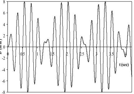
unstable vibrations has been occurred in all methods. Therefore, time step reduces so that each integration could present the quasi exact solution. If time step is 0.0007 second, the NI1, IHOA-1, CA (Newmark Constant Acceleration) and LA (Newmark Linear Acceleration) methods present the quasi exact solution of Figure 10. Regardless the same efficiency, the analysis time of the proposed NI1 scheme is less than other techniques (as described in the portal frame). Furthermore, by reducing time step to 0.0005 second, the previous integrations (NI1, IHOA-1, CA and LA); the NI5 and IHOA-5 also lead to the quasi exact solution. When time step is 0.0004 second, all methods can present the quasi exact response except the IHOA-2, 3 and NI2, 3; however smaller time steps such as 0.0003 second solve this problem. These analyses show that the first, fourth and fifth accuracy order of the proposed integration (NI1, NI4 and NI5) have more ability than other orders. Undamped vibrations which do not appear in real systems cause a few reduction in efficiency of the N-IHOA. Moreover, this example shows that the proposed time integration can be successfully used for dynamic analysis of systems which are modeled by finite differences methods.

Wide range of dynamic analyses performed here clearly state that the numerical accuracy is different with the mathematical accuracy. From the mathematical point of view, it is expected that by increasing the accuracy order, the more accurate results are obtained. In practice, this behavior does not always happen. For example, the second and third order schemes of the proposed integration have not suitable efficiency in numerical examples compared with the first, forth and fifth order methods. Some reasons could be presented for this subject such as, the lack of formulations in using the Taylor expansion and the inverse expansion which are the approximation methods (not exact), the effect of numerical errors and etc.

-8 -6 -4 -2 0 2 4 6 8

0 0.5 1 1.5 2 2.5 3 3.5 4

t (sec)

D

(mm)

Figure 10. Tip displacement of the Euler beam

5. CONCLUDING REMARKS

The new implicit higher order accuracy method i.e. the N-IHOA technique was proposed for numerical dynamic analysis under the assumption of constant time step. Utilizing both velocity and acceleration vectors of previous time steps for integrating the dynamic equation of motion is the main originality of the suggested method compared with other techniques such as the IHOA scheme. These formulations were followed by a comprehensive study on the mathematical accuracy order and the stability condition of the proposed method. From the mathematical point of view, it proves that the new multi time step integration is conditionally stable and the displacement’s accuracy of the N-IHOA scheme is one order less than the displacement formulated by the IHOA method. It should be noted that both methods present the velocity vector by the same mathematical accuracy order. However, simplicity, lower computational efforts and lower requirement memory are the main advantageous of the proposed integration compared with the IHOA method. The reason for this subject is that the new method runs with only one set of weighted factors; however the IHOA technique requires two groups of different values. Wide range of numerical dynamic analyses also show that by a similar time step, the numerical accuracy of the proposed method is higher than the common methods such as the Wilson-θ and the Newmark-β schemes. Moreover, it is proved numerically that the proposed integration with accuracy orders 4 (NI4) and 5 (NI5) have the best efficiency in all examples.

6. REFERENCES

1. Chung, J. and Hulbert, G., “A time integration method for structural dynamics with improved numerical dissipation: the generalized α-method”, Journal of Applied Mechanics, Vol. 30, (1983), 371-384.

2. Hibler, H.M., Hughes, T.J.R. and Taylor, R.L., “Improver numerical dissipation for time integration algorithm in structural dynamics”, Earthquake Engineering and Structural Dynamics, Vol. 5, (1977), 283-292.

3. Wood, W.L., Bossak, M. and Zienkiewicz, O.C., “A alpha modification of Newmark’s method” International Journal for numerical methods in Engineering, Vol. 15, (1981), 1562-1566.

4. Kim, S.J., Cho, J.Y. and Kim, W.D., “From the trapezoidal rule to higher order accurate and unconditionally stable time-integration method for structural dynamics”, Computer

Methods in Applied Mechanics and Engineering, Vol. 149,

(1997), 73-88.

5. Fung, T.C., “Third order time-step integration methods with controllable numerical dissipation”, Communications in Numerical Methods in Engineering, Vol. 13, (1997), 307-315. 6. Fung, T.C., “Complex-time step newmark methods with

7. Tamma, K.K., Zhou, X. and Sha D., “A Theory of development and design of generalized integration operators for computational structural dynamics”, International Journal for numerical methods in Engineering, Vol. 50, (2001), 1619-1664.

8. Modak, S. and Sotelino, E., “The generalized method for structural dynamic applications”, Advances in Engineering Software, Vol. 33, (2002), 565-575.

9. Mancuso, M. and Ubertini, F., “The Nørsett time integration methodology for finite element transient analysis”, Computer

Methods in Applied Mechanics and Engineering, Vol. 191,

(2002), 3297-3327.

10. Bathe, K.J. and Baig, M.M.I., “On a composite implicit time integration procedure for nonlinear dynamics”, Computers and

Structures, Vol. 83, (2005),2513-2524.

11. Keierleber, C.W. and Rosson, B.T., “Higher-Order Implicit Dynamic Time Integration Method”, Journal of Structural

Engineering ASCE, Vol. 131-8, (2005), 1267-1276.

12. Bathe, K.J., “Conserving energy and momentum in nonlinear dynamics: A simple implicit time integration scheme”, Computers and Structures, Vol. 85, (2007), 437-445.

13. Soares, D. and Mansur, W.J., “A frequency-domain FEM approach based on implicit Green’s functions for non-linear dynamic analysis”, International Journal of Solids and Structures, Vol. 42-23, (2005), 6003-6014.

14. Loureiro, F.S. and Mansur, W.J., “A novel time-marching scheme using numerical Green’s functions: A comparative study for the scalar wave equation”, Computer Methods in

Applied Mechanics and Engineering, Vol. 199, (2010),

1502-1512.

15. Wang, M.F. and Au, F.T.K., “Precise integration methods based on Lagrange piecewise interpolation polynomials”,

International Journal for Numerical Methods in Engineering,

Vol. 77, (2009), 998-1014.

16. Rezaiee-Pajand, M. and Alamatian, J., “Implicit higher order accuracy method for numerical integration in dynamic analysis”, Journal of Structural Engineering, ASCE, Vol. 134-136, (2008), 973-985.

17. Liu, T., Zhao, C., Li, Q. and Zhang, L, “An efficient backward Euler time-integration method for nonlinear dynamic analysis of structures”, Computers and Structures, Vol. 106-107, (2012), 20-28.

18. Hulbert, G. and Chung, J., “Explicit time integration algorithm for structural dynamics with optimal numerical dissipation”,

Computer Methods in Applied Mechanics and Engineering,

Vol. 137, (1996), 175-188.

19. Hoff, C. and Taylor, R.L., “Higher derivative explicit one step methods for non-linear dynamic problems. Part I: Design and theory”, International Journal for Numerical Methods in Engineering, Vol. 29, (1990), 275-290.

20. Katona, M. and Zienkiewicz, O.C., “A unified set of single step algorithms Part 3: The beta-m method, A generalization of the Newmark scheme”, International Journal for Numerical

Methods in Engineering, Vol. 21, (1985), 1345-1359.

21. Rostami, S., Shojaee, S. and Moeinadini, A., “A parabolic acceleration time integration method for structural dynamics using quartic B-spline functions”, Applied Mathematical Modeling, (2011), in press.

22. Zhai, W.M., “Two simple fast integration methods for large-scale dynamic problems in engineering,” International Journal

for numerical methods in Engineering, Vol. 39, (1996),

4199-4214.

23. Rezaiee-Pajand, M. and Alamatian, J., “Numerical time integration for dynamic analysis using new higher order predictor-corrector method”, Journal of Engineering

Computations, Vol. 25-26, (2008), 541-568.

24. Alamatian, J. and Rezaeepazhand, J., “A simple approach for etermination of actuator and sensor locations in smart structures subjected to the dynamic loads”, International Journal of

Engineering, Vol. 24, No. 4, (2011), 341-349.

25. Pena, J.M., “Characterizations and stable tests for the Routh-Hurwitz conditions and for total positivity”, Linear Algebra and its Applications, Vol. 393, (2004), 319-332.

26. Rezaiee-Pajand, M. and Alamatian, J., “Nonlinear dynamic analysis by Dynamic Relaxation method”, Journal of Structural Engineering and Mechanics, Vol. 28-5, (2008), pp. 549-570.

27. Mickens, R.E., “A numerical integration technique for conservative oscillators combining non-standard finite differences methods with a Hamilton’s principle”, Journal of Sounds and Vibrations, Vol. 285, (2005), 477-482.

28. Liu, Q., Zhang, J. and Yan, L., “A numerical method of calculating first and second derivatives of dynamic response based on Gauss precise time step integration method”,

European Journal of Mechanics A/Solids, Vol. 29, (2010),

370-377.

29. Felippa, C.A., “Nonlinear Finite Element Methods”, <http:// www.colorado.edu /courses.d /nfemd/> (Feb. 10 2002). 30. Paz, M., “Structural Dynamics: Theory and Computation”,

A Modified Multi Time Step Integration for Dynamic Analysis

J. Alamatian

Civil Engineering Department, Mashhad Branch, Islamic Azad University, Mashhad, Iran, 91735-413

P A P E R I N F O

Paper history:

Received 7 June 2012

Received in revised form 18 July 2012 Accepted 30 August 2012

Keywords: Dynamic Analysis Implicit Multi Time Step Higher Order Integration

هﺪﯿﮑﭼ

دزادﺮﭘﯽﻣ،ﺖﺑﺎﺛﯽﻧﺎﻣزمﺎﮔﺎﺑﯽﮑﯿﻣﺎﻨﯾدﻞﯿﻠﺤﺗياﺮﺑﺪﯾﺪﺟﯽﻣﺎﮔﺪﻨﭼﯽﻨﻤﺿﻪﯿﻟواﻊﺑﺎﺗﮏﯾﻪﺑ،ﻪﻟﺎﻘﻣﻦﯾا .

ﯽﻣشورﻦﯾاﺎﺑ

داددﻮﺒﻬﺑارزﺎﯿﻧدرﻮﻣﻪﻈﻓﺎﺣندﻮﺑدﺎﯾزوتﺎﺒﺳﺎﺤﻣيﻻﺎﺑﻢﺠﺣ،ﯽﻨﻌﯾﯽﻣﺎﮔﺪﻨﭼيﺎﻬﺷوريﺎﻬﯿﺘﺳﺎﮐﻦﯾﺮﺘﻤﻬﻣناﻮﺗ .

ياﺮﺑ

ونﺎﮑﻣﺮﯿﯿﻐﺗيﺎﻫرادﺮﺑيﺮﯿﮔﻪﯿﻟواﻊﺑﺎﺗياﺮﺑ،ﺐﯿﺗﺮﺗﻪﺑﻪﺘﺷﺬﮔﯽﻧﺎﻣزمﺎﮔﻦﯾﺪﻨﭼبﺎﺘﺷوﺖﻋﺮﺳيﺎﻫرادﺮﺑ،رﻮﻈﻨﻣﻦﯾا ﺪﻧﻮﺷﯽﻣهدﺎﻔﺘﺳايرﺎﺟﯽﻧﺎﻣزمﺎﮔﺖﻋﺮﺳ .

ﺎﻫﻪﻄﺑارردارﯽﻧزوﻞﻣﺎﻋﻪﺘﺳدﮏﯾﺎﻬﻨﺗيﺪﻨﯾاﺮﻓﻦﯿﻨﭼ،دادنﺎﺸﻧناﻮﺗﯽﻣ

ﺎﺣوتﺎﺒﺳﺎﺤﻣﻢﺠﺣﻪﮐياﻪﻧﻮﮔﻪﺑ؛ﺪﻨﮐﯽﻣدراو ﯽﻣﺎﮔﺪﻨﭼيﺎﻬﺷورﺎﺑﻪﺴﯾﺎﻘﻣرد،يدﺎﻬﻨﺸﯿﭘﻪﯿﻟواﻊﺑﺎﺗزﺎﯿﻧدرﻮﻣﻪﻈﻓ

ﺪﺷﺎﺑﯽﻣﺮﺘﻤﮐ،ﺪﻨﻨﮐﯽﻣهدﺎﻔﺘﺳاﺖﻗدويراﺪﯾﺎﭘﺶﺠﻨﺳياﺮﺑﯽﻧزوﻞﻣﺎﻋهوﺮﮔﻦﯾﺪﻨﭼزاﻪﮐﻪﺑﺎﺸﻣ .

ﯽﯾﺎﻬﯿﮔﮋﯾو،ﻦﯾاﺮﺑﺎﻨﺑ

ﯿﻠﺤﺗرداريدﺎﻬﻨﺸﯿﭘﻪﯿﻟواﻊﺑﺎﺗﯽﯾارﺎﮐ،زﺎﯿﻧدرﻮﻣكﺪﻧاﻪﻈﻓﺎﺣوﻢﮐتﺎﺒﺳﺎﺤﻣ،ﯽﮔدﺎﺳﺪﻨﻧﺎﻣ ﺮﯿﻏﯽﮑﯿﻣﺎﻨﯾدﻞ

ﻪﻧﺎﻣﺎﺳﯽﻄﺧ

ﺪﻫدﯽﻣﺶﯾاﺰﻓاگرﺰﺑيﺎﻫ .

توررﺎﯿﻌﻣورﻮﻠﯿﺗﻂﺴﺑ،ﺎﺠﻨﯾارد

-ﻦﯿﯿﻌﺗوﯽﻧزويﺎﻬﻠﻣﺎﻋﻪﺒﺳﺎﺤﻣياﺮﺑﺐﯿﺗﺮﺗﻪﺑ،ﺰﺘﯾورﺎﻫ

ﺪﻧورﯽﻣرﺎﮐﻪﺑﻪﯿﻟواﻊﺑﺎﺗيراﺪﯾﺎﭘهدوﺪﺤﻣ .

ﻞﻣﺎﺷﯽﮑﯿﻣﺎﻨﯾدﻪﻧﺎﻣﺎﺳﺪﻨﭼ،ﺪﯾﺪﺟيزﺎﺳﻪﻄﺑاريدﺪﻋﯽﯾارﺎﮐﯽﺳرﺮﺑياﺮﺑ

اﺮﯿﺗولﺎﺗﺮﭘبﺎﻗ،ﯽﻄﺧﺮﯿﻏنﺎﺳﻮﻧ ﺪﻧﻮﺷﯽﻣﻞﯿﻠﺤﺗﺮﻠﯾو

. ﺖﻋﺮﺳوﺖﻗد،نﺎﺴﮑﯾﯽﻧﺎﻣزمﺎﮔﮏﯾﺎﺑ،ﺪﻨﻫدﯽﻣنﺎﺸﻧﺞﯾﺎﺘﻧ

كرﺎﻣﻮﯿﻧيﺎﻫهﻮﯿﺷﺪﻨﻧﺎﻣلواﺪﺘﻣيﺎﻬﺷورزاﺮﺘﺸﯿﺑيدﺎﻬﻨﺸﯿﭘشور

-نﻮﺴﻠﯾو،ﺎﺘﺑ -ﺮﮕﯾدﯽﻣﺎﮔﺪﻨﭼيﺎﻬﺷورزاياهرﺎﭘوﺎﺘﺗ

ﺪﺷﺎﺑﯽﻣ .