A Robust Model for a Dynamic Cellular Manufacturing System with Production Planning

(1)

International Journal of Engineering

J o u r n a l H o m e p a g e : w w w . i j e . i r

A Robust Model for a Dynamic Cellular Manufacturing System with Production

Planning

R. Tavakkoli-Moghaddam* a_{, M. Sakhaii} b_{, B. Vatani} c

a_{School of Industrial Engineering, College of Engineering, University of Tehran, Tehran, Iran} b_{Department of Industrial Engineering, University of Tabriz, Tabriz, Iran}

c_{Department of Electrical Engineering, Semnan University, Semnan, Iran}

P A P E R I N F O

Paper history: Received 28 March 2013

Received in revised form 12 September 2013 Accepted 14 September 2013

Keywords:

Robust Optimization Cell Formation Inter-cell Design Production Planning Uncertainty

A B S T R A C T

This paper develops a robust optimization approach for a dynamic cellular manufacturing system (DCMS) integrated with production planning under uncertainty of parts processing time. To deal with this uncertainty, a robust optimization as a tractable approach is adopted. The model includes cell formation, inter-cell layout and production planning concepts under a dynamic environment. The aim of the model is to minimize inter and intra-cell material handling, inventory holding, back order and reconfiguration costs. To verify the behavior of the presented model and the performance of the developed approach, a numerical example solved in finding an optimal solution.

doi:10.5829/idosi.ije.2014.27.04a.09

NOMENCLATURE

Decision variables h

i

B Backorder of part type i in period h ( 0 ₀ i

B = ) Indices

h i

I Inventory of part type i at the end of period h ( 0 ₀ i

I = ) c c, ¢ Index for machine cells (c=1,...,C)

,

h m c

N ìí1 if machine type m is located in cell in period h;_{0 otherwise} î

c

h Index for production periods (h=1,...,H)

h i

PQ Production quantity of part type i to be produced in period h i Index for parts (i=1,...,I)

h i

PQB 1 if 0

0 otherwise

h i PQ

ì > ü

ï ï

í ý

ï ï

î þ j Index of different decision variables

,

l l¢ Index for a candidate locations to be a cell (l=1,...,L) _M Number of machines

m Index for machines (m=1,...,M) R_ih Number of available routings for part type i in period h

n Index of different constraints ,

h i m

t Processing time of part i on machine m in period h

r Index for routings required by part i in period h (r=1,...,R_ih) h_, i m

t

% Uncertain processing time of part _h i on machine m in period

n

t Uncertain element of the n-th constraint (1£ £n CN) adopting

values from truncated uncertainty interval ,

h i m

t

$ Range of uncertain processing time of part _{in period}_h i on machine m

{

(1) (2) (3) ( ,)

}

,, , , , ,..., ,r i

K r i r i r i r i

U U U U Machine index in routing r of part type i th m¢, Time-capacity of machine type m in period h

(2)

Input parameters Indices

1

A Inter-cell part trip unit cost UPc Maximum number of machines should be located in cell c

2

A Intra-cell part trip unit cost h

i

a Unit holding cost of part type i in period h

A¥ A large positive quantity bih Unit backorder cost of part type i in period h

%n j,

a Uncertain element of the n-th row and the j-th column in A gm Relocation cost of machine m between production periods

, n j

a Estimated nominal value of a%n j, Gn

Conservation level value for the n-th constraint (

1£ £n CN)

$n j,

a Estimated range of a%n j, Jn Number of elements of Jn

C Number of machine cells should be constructed Sn Number of elements of Sn

CN Total number of Constraints Matrices and Vectors

h

D_i Demand value for part i in period h A CN DN´ matrix of coefficients

,

l l

Dis ¢ Distances between two candidate locations landl¢ X DN-dimensional decision vector

DN Total number of decision variables Sets

H Number of production periods Jn

Set of uncertain elements of the n-th constraint (

1£ £n CN)

I Number of parts Sn

Set of uncertain elements of either objective function (n=0) or n-th constraint (1£ £n CN) adopting values from a respective uncertainty interval

, h r i

K Number of machines in routing r of part type i in period h Variables

L Number of candidate locations to be a cell (L C³ ) p y z, , _{Continuous auxiliary robust modeling variables}

c

Low Minimum number of machines should be located in cell c xj Element of the j-th row in X

, h r i

V 1 if routing of part type is selected as process plan in period ;

0; otherwise ì

í î

r i h

,

h c l

X ìí1 if cell is to be constructed in location in period ;_{0 otherwise} î

c l h

1. INTRODUCTION

Today’s industrial world witnesses an increasing global competition, where old technologies failed to overcome the new form of change in demand. The application of group technology to production systems has in industries led to the introduction of cellular manufacturing (CM) which tries to take advantage of the similarity between parts. Each CMS design is consisted of four important decisions; namely cell formation (CF), group layout (GL), group scheduling (GS) and resource allocation [1], in which most of studies have developed CF problems [2, 3]. Only a few studies have concentrated on integrating two or more CMS decisions. Kia et al. [4] proposed an integration of CF and GL models considering the multi-rows layout utilization to locate machines in the cells configured with flexible shapes and several design features (e.g., alternative process routings, operation sequence, processing time, production volume of parts, purchasing machine, duplicate machines, machine capacity, lot splitting, intra-cell layout, inter-cell layout, multi-rows layout of equal area facilities and flexible reconfiguration). Jolai et al. [5] considered the integration of CL and GL models and proposed an

electromagnetism-like algorithm to solve the problem. Arkat et al. [6] proposed a model that integrates CF, GL and cellular scheduling to minimize the total movement and completion time of parts. Their results show that considering three CM decisions simultaneously can significantly improve the performance of CM systems.

(3)

considering worker flexibility. In most studies related to CMS under a dynamic environment, input parameters are considered deterministic and certain. While in reality, a number of parameters (e.g., processing time, part demand, product mix, inter-arrival time and available machine capacity) are uncertain. Mahdavi et al. [10] developed the multi-period cell formation and production planning in a DCMS considering worker assignment. The objective of the model is to minimize machine, reconfiguration, inter-cell material handling, inventory holding, backorder, worker hiring, firing and salary costs.

Some studies of considering uncertainty are as follows. Szwarc et al. [11] considered uncertainty in demand and machines capacity in CMS problem, and is resolved by fuzzy approach. Tavakkoli-Moghaddam et al. [12] proposed a multi-objective model for a cell formation problem under fuzzy and dynamic conditions, the main goal of the proposed model was to select a process plan with the minimum cost and also to identify the most appropriate production volume with respect to fuzzy demands and capacities.Asgharpour and Javadian [13] presented a nonlinear integer CMS model in dynamic and stochastic states solved by a genetic algorithm (GA) and considered a dynamic production, a stochastic demand, routing flexibility and machine flexibility.

Tavakkoli-Moghaddam et al. [14] developed a model for facility layout problem in CMS with stochastic demands, where the aim of objective function is to minimize inter-cell and intra-cell costs. Ghezavati and Saidi-Mehrabad [15] proposed a CM model and assumed that processing and arrival times for parts are stochastic. After formulating the problem with queuing theory, it was solved with new combination of the GA and simulated annealing (SA) algorithm. In addition, Ghezavati and Saidi-Mehrabad [16] applied a scenario-based stochastic programming technique to solve the CF problem integrated with GS decision. Rabbani et al. [17] proposed a bi-objective cell formation problem with stochastic demand quantities and solved with a two-phase fuzzy linear programming approach. Studies considering uncertainty can be categorized to four approaches: stochastic programming approach, fuzzy

programming approach, stochastic dynamic

programming approach, and robust optimization approach [18, 19]. Fuzzy optimization (FO) is an alternative method to cope with uncertainty that represents uncertainty through fuzzy numbers. Its aim is to find the best decision alternative under a membership to a given set that is inexact. On the other hand, stochastic programming (SP) is a methodology for solving optimization problems under uncertainty, which is usually characterized by a probability distribution on some parameters. In other words, a scenario generation approach is used to produce some scenarios from a

probability distribution representing realizations of random variables associated with uncertain sources.

In real-world applications of linear programming (LP), there is the possibility that uncertainty in the input parameters may make the usual optimal solution no longer optimal or even infeasible. Therefore, the need to use approaches, which are immune to data uncertainty, increases. A recent methodology for optimization under uncertainty is robust optimization that models data uncertainties through a set of deterministic and bounded intervals [20]. The robust optimization approach solves a deterministic version of the original uncertain problem to obtain an optimal solution that is immunized against data uncertainties [21].

It is proved that the RO method outperforms other FO and SO methods. The main advantages of this method can be described as follows:

· Many FO methods increase the solving complexity and are typically difficult to be solved in a reasonable computational time, especially in comparison with the proposed RO method that is less sophisticated.

· Standard approaches (e.g., RO), which utilizes real-valued quantities, are less difficult to understand than fuzzy optimization using fuzzy numbers.

· In scenario-based SP methods, a number of scenarios may be huge and can increase the model complexity strictly. However, the RO method remains computationally tractable irrespectiveness of its number of uncertain parameters [22, 23]. In this paper, a robust optimization approach is proposed for the integrated mathematical model of cell formation, inter-cellular layout and production planning with alternative process routing under a dynamic environment to minimize the presented model against the product processing time uncertainty. The aim of the objective function is to minimize inter-cell, intra-cell, inventory holding, back order and machine reconfiguration costs.

This paper is organized as follows. In section 2, the mathematical programming model is presented. Section 3 presents an example with computational results to demonstrate the behavior of the presented model and verify the performance of the developed approach. The paper ends with conclusion.

2. PROPOSED FORMULATION

(4)

for each part are also considered; where for one part, one of its routings with the lowest cost is chosen among other routings. Then, the presented nonlinear model is linearized and afterwards a robust optimization approach is applied throughout the model as a tractable optimization technique to cope with the product processing time uncertainty.

The problem is formulated according to the following assumptions:

·The demand for each part type in each period is known and deterministic.

·Parts have different processing routings where each routing has different sequence of machines.

·Inter-cell movement cost is dependent on the distance traveled, while intra-cell movement cost is regardless of the distance.

·The inventory holding and back orders are considered.

·The time capacity of each machine type is known.

·The upper and lower bound of cell size is known.

2. 1. Mathematical Model

, 1

1

, ,

1 ,

1 1 1 1 1 1 1 1

, , , , ,

M in .

. . . . . h h r i i m m

r i r i

K R

H I C C L L

l l h i r m c c l l

h h h h h h

r i i U c c l U c c l

A Dis

V P Q N X N X

-+ ¢ ¢ ¢ = = = = = = = = ¢ ¢ ¢ .

å å å å å å å å

(1a)

, 1

1

, ,

2 , , ,

1 1 1 1 1

. . . .

h r i i

m m

r i r i

K R

H I C

h h h h r i i U c U c h i r i c

A V PQ N N

-+

= = = = =

+

ååå å å

(1b)

1 1 . H I h h i i h i I a = =

+

åå

(1c)

1 1 . H I h h i i h i B b = =

+

åå

+ (1d)

1

1 1

, , , , ,

1 1 1 1 1 1

. . . . .

H M C C L L

h h h h m m c m c c l c l l l h m c c l l

N N X X Dis

g -+ + ¢ ¢ ¢ ¢ ¢ ¢ = = = = = =

åååååå

(1e) s.t. , 1 , M h

m c c m

N Low h c

= ³ "

å

(2) , 1 , M h m c c m

N UP h c

=

£ "

å

(3) , 1 1 , C h m c c

N h m

=

= "

å

(4) , 1 , h i R h h

r i i r

V PQB h i

=

= "

å

(5) , 1 1 , L h c l l

X h c

=

= "

å

(6) , 1 1 , C h c l c

X h l

=

£ "

å

(7) , , , , 1 1 . . , h i m r i R I

h h h r i i i U h m i r

V PQ t t h m

= =

¢

£ "

åå

(8)

1 1 _,

h h h h h h i i i i i i

PQ ₌D _-I - ₊B - ₊I _-B _"h i

(9)

. ,

h h

i i

PQ £A PQB¥ "h i (10)

, (0,1) , ,

h m c

N Î "h m c (11)

, (0,1) , ,

h c l

X Î "h c l (12)

(0,1) ,

h i

PQB Î "h i (13)

, (0,1) , ,

h r i

V Î "h r i (14)

, , 0 and int. ,

h h h i i i

PQ I B ³ "h i (15)

The objective function (OF) of the presented model consists of five terms as follows. Equation (1a) represents the inter-cell material handling cost where, this cost happens when parts need to be processed in more than one cell. In Equation (1b), the intra-cell material part trip occurs only when two consecutive operations in one routing are allocated to the same cell but to different machines. Equation (1c) represents the inventory holding cost which happens due to keeping inventories for all parts. In Equation (1d), the backorder cost occurs when the manufacturing system is unable to fill an order and must complete it later. Equation (1e) represents the relocation cost of machines between periods where the distance between cells for these reconfigurations are considered. Equations (2) and (3) ensure that the number of machines for one cell is not exceeded lower and upper bound of cell size. The lower bound is used to prevent all machines from being assigned to a single cell.

(5)

particular period can be a positive quantity only when its corresponding binary viable is equal to 1. At last, Equations (11) to (15) are to define the decision variables types.

2. 2. Linearization In this section, the linearization of the nonlinear model is developed based on linearization methods [4, 24]. The nonlinearity of the model is due to Equations (1a), (1b) and (1e) and (8). Therefore, to linearize the model, some new variables should be defined as follows:

, . ,

h h h

r i i r i

VPQ =PQ V

1 1

,, , , , . ,, . , ,

m m m m

r i r i r i r i

h h h h

r i

U U c VPQ NU c NU c

y + = +

1 1

,, , , , , , , . ,, . , , . ,. ,

m m m m

r i r i r i r i

h h h h h h

r i c l c l

U c l U c l VPQ NU c NU c X X

j + _{¢ ¢}= + _¢ _{¢ ¢}

1 1

, , , , , . , . , . ,

h h h h h

m c c l l Nm c Nm c Xc l Xc l

h + +

¢ ¢ = ¢ ¢ ¢

The following equations respect to new variables must be added to the original model:

(

)

, . 1 , , ,

h h h

r i i r i

VPQ ³PQ -A¥ -V "h r i (16)

, 0 and int. , ,

h r i

VPQ ³ "h r i (17)

(

)

1 1

,, , , , . 2 ,, , ,

m m m m

r i r i r i r i

h h h h

r i

U U c

VPQ

A

N

U c

N

U c

y

+ ³ - _¥ - - +

, , , , h r i m c

"

(18)

1

,, , , 0 and int. , , , ,

m m r i r i h

U U c h r i m c

y + ³ " (19)

(

1 1

,, , , , , , , . 4 ,, , ,

m m m m

r i r i r i r i

h h h h

r i

U c l U c l

VPQ

A

N

U c

N

U c

j

+ _{¢ ¢}³ - _¥ - - + _¢

)

, , , , , , , , ,

h h c l c l

X X _{¢ ¢} h r i m c c l l¢ ¢

- - "

(20)

1

,, , , , , , 0 and int. , , , , , , ,

m m r i r i h

U c l U c l h r i m c c l l

j + _{¢ ¢} ³ " ¢ ¢ (21)

1 1

, , , , , , , ,

4 h h h h h

h + +

¢ ¢ £ + ¢+ + ¢ ¢

1,..., 1, , , , , h H m c c l l¢ ¢

" = - (22)

1 1

, , , , , , , , 3

h h h h h

h + +

¢ ¢³ + ¢+ + ¢ ¢

-1,..., 1, , , , , h H m c c l l¢ ¢

" = - (23)

, , , , is bin. , , , , ,

h

m c c l l h m c c l l

h ¢ ¢ " ¢ ¢ (24)

By substituting new variables in the model, the linear form of the model is as follows:

, 1

1

, ,

1 , , , , , , 1 1 1 1 1 1 1 1

Min . .

h h

r i i

m m

r i r i

K R

H I C C L L

h

l l U c l U c l h i r m c c l l

A Dis j

-+

¢ ¢ ¢

¢ ¢

= = = = = = = =

ååå å åååå

, 1

1

, ,

2 , ,

1 1 1 1 1

. h h r i i m m r i r i K

R

H I C

h U U c h i r m c

A y

-+ = = = = =

+

ååå å å

(25)

1

, , , , , 1 1 1 1 1 1

. .

H M C C L L h

m m c c l l l l h m c c l l

Dis g h -¢ ¢ ¢ ¢ ¢ = = = = = = +

åååååå

1 1 . H I h h i i h i I a = = +

åå

1 1 . H I h h i i h i B b = =

+

åå

s.t.

Equations (2) to (7), (9) to (15), (16) to (24)

, , , , 1 1 . , h i m r i R I h h r i i U h m i r

VPQ t t h m

= =

¢

£ "

åå

(26)

2. 2. Robust Optimization Approach In recent years, dealing with uncertain data is a major challenge in optimization. One approach to address data uncertainty is developed under the name of robust optimization, which means finding a solution that can cope best with all possible realizations of the uncertain data. Various approaches of robust optimization are developed. Idea behind robust optimization is to consider the worst case scenario without a specific distribution assumption. The roots of robust optimization can be found in the field of robust control and in the work of Soyster [25] considered a deterministic linear optimization model, which is feasible for all data lying in a convex set. However, the model is very conservative and is protected against the worst-case scenario. Subsequently, a number of important robust formulations are developed by Ben-Tal and Nemirovski [26-28], El Ghaoui et al. [29] and Bertsimas et al. [30].

In this section, we present a robust approach developed by Bertsimas et al. [31] for discrete optimization problems with uncertain parameters based on a polyhedral uncertainty set. Aforementioned studies are based on ellipsoidal uncertainty or box uncertainty sets. The approach proposed by Bertsimas et al. [31] is adopted according to the following justifications:

·The robust optimization (RO) model proposed by Bertsimas [31] is more tractable than RO frameworks with ellipsoidal uncertainty sets. A robust counterpart of a model considering uncertain linear programming (LP) with ellipsoidal uncertainty sets is solved in form of second-order conic programming (SOCP). However, the robust counterpart of this model with polyhedral uncertainty sets remains in form of linear programming. Besides, obtaining a solution from SOCP as a non-linear model is more difficult than LP. Then, it is not particularly attractive for solving robust discrete optimization problems[31, 32].

(6)

flexiblely than RO with a box uncertainty set (e.g., Soyster’s RO [25]). Since RO with polyhedral uncertainty offers can assign each conservation level to each uncertainty, RO with a box uncertainty assigns only one conservation level to all uncertainties of each equation [31].

Bertsimas approach permits to control the conservatism level of the solution [31]. Solutions obtained from robust optimization approach guarantees more situations even worst ones. The important concern of the robust methodology in this paper is to present an optimal planning that is robust with regard to data uncertainties in product processing time. The deterministic compact form of the model can be rewritten as follows:

.

T

Min c x s.t.

. A x b£

lb x ub£ £

(27)

Suppose that only matrix A=(an j, ) elements are

subjected to data uncertainty, the RO methodology models data uncertainties through bounded intervals designated as uncertainty set. Therefore, the matrix A’s uncertain elements can be defined using the mean value and range of each uncertain element as follows:

%n j, _{n j}_, $n j, , _{n j}_, $n j, %n j,

a =é_ëa -a a +a ù_û a Î A (28)

A number named conversion level (CL), symbolized by

n

G (n= 0,1,…,CN) is introduced in [31] for robustness intentions and adjusting the robustness level which adopts different values in the interval é_ë0,J_n ù_û

, where Jn

is a set comprises uncertain elements of the n_-th equation J_n = { j a$n j, > 0 }. Therefore, the robust

counterpart of Equation (27) which is nonlinear can be written as follows:

Min _{c x}T.

s.t.

, .

n j j j

a x

å

{ }

{ max, , \ } $,.

(

)

.$,n. tn n n n n n n n n n n

n j _j _n _n n t SÈt S J SÍ = Gê úë ût J SÎ _{j S}Î a x a x

ì ü

ï ï

+ í + G - Gê úë û ý

ï ï

î

å

þ

n

b n

£ "

lb x ub£ £

(29)

By applying the linearization technique for nonlinear Equation (28), we have:

.

T

Min c x s.t.

, . . ,

n

n j j n n n j n

j j J

a x z p b n

Î

+ G + £ "

å

$ _,

, n j. ,

n n j j n

z +p ³a y "n j JÎ

(30)

j j j

y x y j

- £ £ "

j j j

lb £x £ub "j 0

n

z ³ "n

, 0 ,

n j n

p ³ "n jÎJ

0

j

y ³ "j

Now, a robust DCMS model can be developed by introducing a set of symmetric bounded intervals which represent the uncertainty of the product processing time as follows:

, _, , , _, , , ,

h h

h _h _h

i m _{i m} i m _{i m} i m

t% Î_êé_ët -t$ t +t$ _úù_û "h i m (31)

Therefore, the robust counterpart of the proposed model is as follows:

, 1

1

, ,

1 , , , , , ,

1 1 1 1 1 1 1 1

Min OF . .

h h

r i i

m m

r i r i

K R

H I C C L L

h l l U c l U c l h i r m c c l l

A Dis j

-+

¢ ¢ ¢ ¢ ¢

= = = = = = = =

=

ååå å åååå

, 1

1

, ,

2 , ,

1 1 1 1 1

. h h r i i m m r i r i K

R

H I C

h U U c h i r m c

A y

-+ = = = = =

+

ååå å å

1

, , , , , 1 1 1 1 1 1

. .

H M C C L L h

m m c c l l l l h m c c l l

Dis g h -¢ ¢ ¢ ¢ ¢ = = = = = = +

åååååå

1 1 . H I h h i i h i I a = = +

åå

1 1 . H I h h i i h i B b = =

+

åå

(32)

s.t.

Equations (2-7), (9-15), (16-24)

,

, , , , , ,

1 1 1

, . . h i m r i R I I

h h h

r i i U h m h m i m h m

i r i

h m

VPQ t z p t

= = =

"

¢ + G + £

åå

å

(33)

, , _, , , , 1 . , , h i m h r i m i Ur i R _h

h

i U

h m i m _t

r

z p t y h i m

=

+ ³

å

$ " (34)

, _, , , _, , _,

0 , , ,

h h h

m m m

i Ur i i Ur i i Ur i h

r i

t t t

y VPQ y y h r i m

- £ £ ³ " ₍₃₅₎

, 0 ,

h m

z ³ "h m (36)

, 0 , ,

h i m

p ³ "h i m (37)

However, the dimension of the processing time is equal to H I M L´ ´ ´ . However, note that the processing time for machine min part i and period h is similar in all routings. Therefore, the total number of all uncertain variables of the set is equal to H I M´ ´ . Besides, by considering Equations (28) and (31), it is revealed that n=h×m and G G₁, ₂,...,G_{h m}_´ . Hence, in Equation (33), for each m and h, the number of uncertain set’s elements are equal to the number of parts that machine m produces in period h (i.e. Jn = éë0,Jnù =û ëé0,Ih m, ùû), where,

,

h m

(7)

3. NUMERICAL RESULTS

A numerical example is considered to validate the performance of the presented model, in which eight machine types allocated to two possible cells to process 12 different part types, each having maximum three different routings and with the planning decisions over two time periods. This example is solved using the CPLEX 12.5 solver within GAMS software package on the personal computer 2.3 GHz Intel Core i5 with 4GB of RAM. The information related to the machine capacity, distance between candidate locations and part types are given in Tables 1 to 3, respectively. Table 3 contains the information related to the part sequences, routings, processing time and demand. For instance, part type one with the demand quantity of 95 has two different routings. The first routing consists of three operation sequences that each needs machines 7, 5 and 1, respectively. Furthermore, the minimum and maximum sizes of each cell in terms of machine numbers are assumed to be 2 and 4, respectively.

Based on definition in section 2.3, G G₁, ₂,...,G₁₆

(n=h×m=2×8=16) can vary according to the Table 4. Note that when Gn=0, the Equations will be equivalent

to the deterministic form. By changing G Î é_n _ë0,J_n ù_û

there will be also the flexibility of modifying the robustness of the method pertaining to the conservatism level of the solution. In the mentioned example, we adjust the processing time uncertainty , r im,

h i U

t

$ to equal 50% of the nominal processing time andG =n 0.5´Jn.

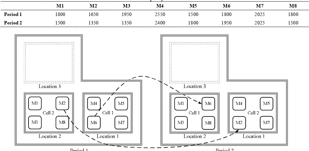
The obtained optimal solution of the proposed integrated model is presented in Tables 5 to 8. The cell configurations for two periods corresponding to the optimal solution of Table 5 are shown in Figure 1.

The optimal inter-cell layout is shown in Table 5. As an example in period one, cells 1 and 2 are constructed in locations 1 and 2, respectively, where they are 1 unit apart. Cell configurations for two periods are also presented in Table 5 and Figure 1. For instance, in period one, machine types M4, M5, M6 and M7 are assigned to cell 1. The efficient routing for each part type is shown in Table 6. By considering Tables 3, 5 and 6, it can be figured out how inter and intra-cell part trips happen. For instance, in period 2, part type 10 needs machines M3, M7 and M6 successively. On the other hand, the machines are assigned to C2, C1 and C1, respectively. Therefore, part type I2 after being processed on M3 in cell C2 would experience inter-cell part trip to cell C1 to be processed on machine M7, at last the part would experience intra-cell trip to M6.

TABLE 1. Distance matrix between cell locations

To

From L1 L2 L3

L1 0 1 2

L2 1 0 1

L3 2 1 0

TABLE 2. Capacity of machines

M1 M2 M3 M4 M5 M6 M7 M8

Period 1 1800 1650 1950 2550 1500 1800 2025 1800

Period 2 1500 1350 1350 2400 1800 1950 2025 1500

(8)

TABLE 3. Input data of part processing

Part Period 1 Period 2

Process Sequence Processing time (min) Demand Process Sequence Processing time (min) Demand

1 M7-M5-M1

M8-M7

2.4-3.2-1.6

4-2.4 95

M8-M5 M8-M7-M1

2.4-3.2

2.4-1.6-0.8 75

2 M2-M5 _M3-M4 0.8-3.2 _1.6-2.4 50 M2-M4-M5 0.8-4-2.4 0

3 M2-M5

M4-M6

2.4-4.8

3.2-4 65

M6-M7 M4-M6 M2-M5-M1

4-1.6 1.6-4 0.8-2.4-1.6

70

4

M1-M7-M8 M7-M4-M8 M1-M4-M3

2.4-4.8-0.8 4.8-3.2-0.8 2.4-3.2-1.6

60 M1-M4-M8 _M4-M7-M1 2.4-3.2-1.6 _4.2-2.4-2.4 50

5 M6-M3-M7

M2-M7-M4

3.2-1.6-0.8

2.4-0.8-1.6 50

M3-M6-M7 M2-M6-M7

3.2-4-0.8

2.4-4-0.8 45

6 M1-M4-M6 _M1-M2-M4 0.8-2.4-1.6 _0.8-1.6-2.4 80 M5-M4-M2 _M6-M7-M3 1.6-1.6-2.4 _0.8-1.6-3.2 60

7 M1-M4-M6

M3-M5-M2

1.6-0.8-2.4

3.2-4-0.8 40

M4-M5-M6 M1-M4-M5

0.8-2.4-3.2

1.6-0.8-2.4 45

8 M3-M7 _M5-M8 _3.2-4.82.4-4 50 M3-M7 _M4-M6 1.6-3.2 _1.6-4.8 60

9 M8-M6-M3

M2-M4-M3

1.6-4.8-6.4

3.2-2.4-6.4 0 M4-M8-M2 1.6-5.6-5.6 90

10 M3-M7-M6

M6-M8

0.8-2.4-1.6

1.6-3.2 50 M3-M7-M6 5.6-4-0.8 45

11 M8-M6-M7 _M2-M4-M3 _3.2-2.4-6.41.6-4-6.4 100 M6-M8-M7 1.6-5.6-5.6 85

12

M1-M7-M4 M4-M8 M1-M5-M4

1.6-3.2-2.4 2.4-4 1.6-2.4-2.4

70

M8-M5-M4 M3-M7-M4 M1-M5-M8

5.7-4-1.6 4.8-4.8-1.6

1.6-4-5.6

75

TABLE 4. Range of variation for conservation levels

Machine Period 1 Period 2

M1 [0,5] [0,5]

M2 [0,7] [0,5]

M3 [0,8] [0,5]

M4 [0,9] [0,8]

M5 [0,6] [0,6]

M6 [0,7] [0,7]

M7 [0,7] [0,9]

M8 [0,7] [0,5]

TABLE 5. Optimal inter-cell layout and machine grouping

Cell Period 1 Period 2

Cell location Machines Cell location Machines

C1 L1 M4,M5,

M6,M7 L2

M1,M8, M3,M6

C2 L2 M3,M8,

M1,M2 L1

M2,M5, M7,M4

TABLE 6. Optimal part routings

1 R2 R2

2 R1 R1

3 R1 R1

4 R1 R1

5 R1 R2

6 R2 R2

7 R2 R1

8 R2 R2

9 R2 R1

10 R2 R1

11 R2 R1

12 R2 R3

TABLE 7. Objective function value (OFV)

OFV Inventory cost Backorder cost Relocation cost Inter-cell cost Intra-cell cost

(9)

TABLE 8. Optimal production plan

Inventory Backorder Production Demand Inventory Backorder Production Demand

1 3 98 95 72 75

2 50 50 0 0

3 65 65 70 70

4 1 61 60 49 50

5 50 50 45 45

6 80 80 60 60

7 45 85 40 0 45

8 50 50 60 60

9 39 39 0 51 90

10 50 50 45 45

11 100 100 7 78 85

12 30 100 70 45 75

TABLE 9. Objective function value (OFV) for 1

7 6

a =

OFV Inventory cost Backorder cost Relocation cost Inter-cell cost Intra-cell cost

3828 404 168 86 1150 2020

TABLE 10. Computational results from different-sized problems

No. I×M×C×H No. variables No. constraints Objective function Computational time (sec) Gap (%)

1 12×8×2×2 2801 7551 3096 106 0

2 18×12×2×2 4973 12467 6453 291 0

3 24×16×2×2 8529 20767 11082 360 0

4 30×20×3×2 13469 41451 31078 914 0

5 36×24×3×2 17793 65519 44736 1159 0

6 42×28×3×2 26858 83587 60981 1453 0.01

7 48×32×4×2 51470 139547 94355 1898 0.01

8 54×36×4×2 97937 259859 135380 2642 0.08

9 60×42×4×2 129911 370775 176901 5648 10.3

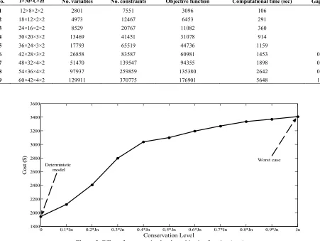
Figure 2. Effect of conservation level on objective function (cost)

0 0.1*Jn 0.2*Jn 0.3*Jn 0.4*Jn 0.5*Jn 0.6*Jn 0.7*Jn 0.8*Jn 0.9*Jn Jn

1800 2000 2200 2400 2600 2800 3000 3200 3400 3600

Conservation Level

C

os

t (

$) Worst case

(10)

The objective function value (OFV) is presented in Table 7. According to mentioned tables, for part type 1 in period 2, its routing R2 is chosen. This part should be processed on machines M8, M7 and M1 allocated to cells C2, C1 and C2, respectively. Hence, this part has two inter-cell trips. Based on the first term of the objective function, its first inter-cell part trip cost, is computed by:

1 2

2 ,1 2,1

2 2 2 2 2 2

1. 2,1. 2,1. 1 U ,2. 2,2. U ,1. 1,1 A Dis V PQ N. X N X

0.85´1´1´72´1´1= 30.6 Note that: 1

2,1

U indicates to machine M8, which is the first machine in the second routing of part type 1. Table 8 demonstrates optimal production planning, demand quantity for each part type can be satisfied through production, backorder and/or inventory. For instance in period 1, the demand of part type 7 is 40 while 85 units are produced. Therefore, 45 units will be kept for next period as inventory and this amount can satisfy the next period’s demand. Furthermore, type part 11 has been produced 78 units while the demand quantity is 85. Therefore, the demand cannot be satisfied completely and 7 units are considered as backorder. To verify the costing effect of inventories, assume that the unit inventory cost of part type 7 is increased from 3 to 6 per unit. Table 9 demonstrates the results in the objective function values. This increase makes the part type 7 demands to be satisfied in each pertaining period, in other words production quantity for part type 7 after this change is 40 and 45 in periods 1 and 2, respectively.

The robust optimization approach by solving the worst case problem presents an optimal solution immunized against all data uncertainties. To verify the behavior of the model, Figure 2 is plotted presenting the effect of the conservation level on the objective function value. According to this figure, the OFV is the function of conservation level. By increasing conservation level, the OFV increases. With robust optimization approach the desire to stay on the safe side can be achieved by enlarging uncertainty set. In the non-presence of conservation level (i.e., deterministic model), the optimal value is 1943. On the other hand, with maximum conservatism (i.e., worst case) the optimal value is increased by 75% to 3409. As far as we increase the conservatism, the presented model becomes more immune against processing time uncertainty. To better illustrate the ability of the robust DCMS model, the computational results from different-sized problems are presented in Table 10 illustrating the computational time, objective function, relative optimality criterion (Gap) and the number of variables and constraints for each problem. It is obvious that by increasing the problem size in terms of a number of variables, the computational time increases. The relative optimality criterion for an MIP problem is as follows:

(

BP BF-

)

/ 1.0

(

e- +10 BF

)

where, BF is the objective function value of the current best integer solution, while BP is the best possible integer solution [33].

4. CONCLUSION

In this paper, a robust optimization approach has been developed for a new presented mathematical model integration of cell formation, inter-cell design, and production planning under dynamic environment, in order to cope with parts processing time uncertainty. This model has minimized inter and intra-cell material handling costs, relocation costs and production planning costs (e.g., inventory and backorder costs). This model has been able to determine the optimal cell configuration and production plan for each part type at each period over the planning horizon. The important advantages of this study are as follows:

· Applying a robust optimization approach to the DCMS.

· Distance-based relocations of machine types.

· Considering different routings for each part type.

· Incorporating inter-cell layout of machines with cell formation to exactly calculate inter-cell material handling cost.

· Considering uncertainty for parts processing time.

For future studies, providing frameworks that which considers more options of uncertainty can be interesting fields.

5. REFERENCE

1. Wemmerlöv, U. and Hyer, N. L., "Procedures for the part family/machine group identification problem in cellular manufacturing", Journal of Operations Management, Vol. 6, No. 2, (1986), 125-147.

2. Chu, C., "Cluster analysis in manufacturing cellular formation", Omega, Vol. 17, No. 3, (1989), 289-295.

3. Singh, N., "Design of cellular manufacturing systems: an invited review", European Journal of Operational Research, Vol. 69, No. 3, (1993), 284-291.

4. Kia, R., Baboli, A., Javadian, N., Tavakkoli-Moghaddam, R., Kazemi, M., and Khorrami, J., "Solving a group layout design model of a dynamic cellular manufacturing system with alternative process routings, lot splitting and flexible reconfiguration by simulated annealing", Computers & Operations Research, Vol. 39, No. 11, (2012), 2642-2658. 5. Jolai, F., Tavakkoli-Moghaddam, R., Golmohammadi, A. and

(11)

6. Arkat, J., Farahani, M. H. and Hosseini, L., "Integrating cell formation with cellular layout and operations scheduling", The International Journal of Advanced Manufacturing Technology, Vol. 61, No. 5-8, (2012), 637-647.

7. Krishnan, K. K., Mirzaei, S., Venkatasamy, V. and Pillai, V. M., "A comprehensive approach to facility layout design and cell formation", The International Journal of Advanced Manufacturing Technology, Vol. 59, No. 5-8, (2012), 737-753. 8. Bulgak, A. A. and Bektas, T., "Integrated cellular manufacturing systems design with production planning and dynamic system reconfiguration", European Journal of Operational Research, Vol. 192, No. 2, (2009), 414-428.

9. Mahdavi, I., Aalaei, A., Paydar, M. M. and Solimanpur, M., "Multi-objective cell formation and production planning in dynamic virtual cellular manufacturing systems", International Journal of Production Research, Vol. 49, No. 21, (2011), 6517-6537.

10. Mahdavi, I., Aalaei, A., Paydar, M. M. and Solimanpur, M., "Designing a mathematical model for dynamic cellular manufacturing systems considering production planning and worker assignment", Computers & Mathematics with Applications, Vol. 60, No. 4, (2010), 1014-1025.

11. Szwarc, D., Rajamani, D. and Bector, C., "Cell formation considering fuzzy demand and machine capacity", The International Journal of Advanced Manufacturing Technology, Vol. 13, No. 2, (1997), 134-147.

12. Tavakkoli-Moghaddam, R., Minaeian, S. and Rabbani, S., "A new multi-objective model for dynamic cell formation problem with fuzzy parameters", International Journal of Engineering—Transactions A: Basic, Vol. 21, No. 2, (2008), 159-172.

13. Asgharpour, M. and Javadian, N., "Solving a Stochastic Cellular Manufacturing Model by Using Genetic Algorithms", International Journal of Engineering Transactions A, Vol. 17, (2004), 145-156.

14. Tavakoli-Moghadam, R., Javadi, B., Jolai, F. and Mirgorbani, S., "An efficient algorithm to inter and intra-cell layout problems in cellular manufacturing systems with stochastic demands", International Journal of Engineering-Materials and Energy Research Center-, Vol. 19, No. 1, (2006), 67.

15. Ghezavati, V. and Saidi-Mehrabad, M., "An efficient hybrid self-learning method for stochastic cellular manufacturing problem: A queuing-based analysis", Expert Systems with Applications, Vol. 38, No. 3, (2011), 1326-1335.

16. Ghezavati, V. and Saidi-Mehrabad, M., "Designing integrated cellular manufacturing systems with scheduling considering stochastic processing time", The International Journal of Advanced Manufacturing Technology, Vol. 48, No. 5-8, (2010), 701-717.

17. Rabbani, M., Jolai, F., Manavizadeh, N., Radmehr, F. and Javadi, B., "Solving a bi-objective cell formation problem with stochastic production quantities by a two-phase fuzzy linear programming approach", The International Journal of Advanced Manufacturing Technology, Vol. 58, No. 5-8, (2012), 709-722.

18. Sahinidis, N. V., "Optimization under uncertainty: state-of-the-art and opportunities", Computers & Chemical Engineering, Vol. 28, No. 6, (2004), 971-983.

19. Mirzapour Al-E-Hashem, S., Malekly, H. and Aryanezhad, M., "A multi-objective robust optimization model for multi-product multi-site aggregate production planning in a supply chain under uncertainty", International Journal of Production Economics, Vol. 134, No. 1, (2011), 28-42.

20. Ben-Tal, A., El Ghaoui, L. and Nemirovski, A., "Robust optimization, Princeton University Press, (2009).

21. Bertsimas, D., Brown, D. B. and Caramanis, C., "Theory and applications of robust optimization", SIAM Review, Vol. 53, No. 3, (2011), 464-501.

22. José Alem, D. and Morabito, R., "Production planning in furniture settings via robust optimization", Computers & Operations Research, Vol. 39, No. 2, (2012), 139-150. 23. Doole, G. J., "Evaluation of an agricultural innovation in the

presence of severe parametric uncertainty: An application of robust counterpart optimisation", Computers and Electronics in Agriculture, Vol. 84, (2012), 16-25.

24. Bagheri, M. and Bashiri, M., "A new mathematical model towards the integration of cell formation with operator assignment and inter-cell layout problems in a dynamic environment", Applied Mathematical Modelling, (2013). 25. Soyster, A. L., "Technical Note—Convex Programming with

Set-Inclusive Constraints and Applications to Inexact Linear Programming", Operations Research, Vol. 21, No. 5, (1973), 1154-1157.

26. Ben-Tal, A. and Nemirovski, A., "Robust convex optimization", Mathematics of Operations Research, Vol. 23, No. 4, (1998), 769-805.

27. Ben-Tal, A. and Nemirovski, A., "Robust solutions of uncertain linear programs", Operations Research Letters, Vol. 25, No. 1, (1999), 1-13.

28. Ben-Tal, A. and Nemirovski, A., "Robust solutions of linear programming problems contaminated with uncertain data", Mathematical Programming, Vol. 88, No. 3, (2000), 411-424. 29. El Ghaoui, L., Oks, M. and Oustry, F., "Worst-case value-at-risk

and robust portfolio optimization: A conic programming approach", Operations Research, Vol. 51, No. 4, (2003), 543-556.

30. Bertsimas, D. and Sim, M., "Robust discrete optimization and network flows", Mathematical Programming, Vol. 98, No. 1-3, (2003), 49-71.

31. Bertsimas, D. and Sim, M., "The price of robustness", Operations Research, Vol. 52, No. 1, (2004), 35-53.

32. Bertsimas, D., Pachamanova, D. and Sim, M., "Robust linear optimization under general norms", Operations Research Letters, Vol. 32, No. 6, (2004), 510-516.

33. CPLEX solver documentation, available at

(12)