Chapter 2
2.1 Let x∈(X\C)∩D. Then x∈X, x ∈D, x6∈C. So x∈D, x 6∈C which gives x∈D\C. Hence (X\C)∩D⊆D\C.
Conversely, if x ∈ D\C then x 6∈ C so x ∈ X\ C , and also x ∈ D. So x∈(X\C)∩D. Hence D\C ⊆(X\C)∩D.
Together these prove that (X\C)∩D=D\C.
2.3 Suppose that x ∈ V. Then x ∈ X and x 6∈ X \V = X ∩U, so x 6∈ U. So x ∈X ⊆Y and x 6∈U, so x ∈Y \U. This gives x∈X∩(Y \U). Hence V ⊆X∩(Y \U).
Conversely suppose that x ∈ X ∩ (Y \ U). Then x ∈ X and x 6∈ U, so x6∈X∩U =X\V. Hence x∈V. This shows that X∩(Y \U)⊆V.
Together these show that V =X∩(Y \U).
2.5 If (x, y) ∈(U1×V1)∩(U2×V2) then x∈U1 and x∈U2 so x∈U1∩U2,
and similarly y∈V1∩V2, so (x, y)∈(U1∩U2)×(V1∩V2). This shows that
(U1×V1)∩(U2×V2)⊆(U1∩U2)×(V1∩V2).
Conversely, if (x, y)∈(U1∩U2)×(V1∩V2) then x∈U1, x∈U2 and y ∈V1, y∈V2
so (x, y)∈U1×V1 and also (x, y)∈U2×V2, so (x, y)∈(U1×V1)∩(U2×V2).
This shows that
(U1∩U2)×(V1∩V2)⊆(U1×V1)∩(U2×V2).
Together these show that
(U1×V1)∩(U2×V2) = (U1∩U2)×(V1∩V2).
2.7 (a) Let the distinct equivalence classes be {Ai : i ∈ I}. Each Ai, being an equivalence class, satisfies Ai ⊆X. To see that the distinct equivalence classes are disjoint, suppose that for some i, j ∈ I and some x ∈X we have x ∈Ai∩Aj. Then for any a∈Ai we have a∼x and x∈Aj, hence a∈Aj. This shows that Ai ⊆Aj. Similarly Aj ⊆Ai. This shows that Ai=Aj. Thus distinct equivalence classes are mutually disjoint. Finally, any x∈X is in some equivalence class with respect to ∼, so X⊆[
i∈I
Ai. Also, since each Ai is a subset of X we have
[
i∈I
Ai ⊆X.
So X=[ i∈I
Ai and the union on the right-hand side is disjoint.
(b) We define x1 ∼ x2 iff x1, x2 ∈ Ai for some i ∈ I. This is reflexive since
each x ∈ X is in some Ai so x ∼ x. It is symmetric since if x1 ∼ x2 then
x1, x2 ∈Ai for some i∈I and then also x2, x1 ∈Ai so x2 ∼x1. Finally it is
transitive since if x1 ∼x2 and x2 ∼x3 then x1, x2 ∈Ai for some i∈ I and
x2, x3∈Aj for some j∈I. Now x2 ∈Ai∩Aj and since Ai∩Aj =∅ for i6=j we must have j = i. Hence x1, x3 ∈ Ai and we have x1 ∼ x3 as required for
Chapter 3
3.1 Suppose that y ∈ f(A). Then y = f(a) for some a ∈ A. Since A ⊆ B, also a ∈ B so y = f(a) ∈ f(B). By definition f(B) ⊆ Y. This shows that f(A)⊆f(B)⊆Y.
Suppose that x ∈ f−1(C). Then f(x) ∈C, so since C ⊆ D we have also that f(x) ∈ D. Hence x ∈ f−1(D). By definition f−1(D) ⊆ X. This shows that f−1(C)⊆f−1(D)⊆X.
3.3 First suppose that x ∈ (g ◦f)−1(U), so g(f(x)) = (g◦f)(x) ∈ U. Hence by definition of inverse images f(x)∈g−1(U) and again by definition of inverse images x∈f−1(g−1(U)). This shows that (g◦f)−1(U)⊆f−1(g−1(U)).
Now suppose that x∈f−1(g−1(U)). Then f(x)∈g−1(U), so g(f(x))∈U, that
is (g◦f)(x) ∈ U, and by definition of inverse images, x ∈ (g◦f)−1(U). Hence f−1(g−1(U))⊆(g◦f)−1(U).
These together show that (g◦f)−1(U) =f−1(g−1(U)).
3.5 We know from Proposition 3.14 in the book that if f : X → Y is onto then f(f−1(C)) =C for any subset C of Y.
Suppose that f :X → Y is such that f(f−1(C)) =C for any subset C of Y.
For any y ∈ Y we can put C = {y} and get that f(f−1(y)) = {y}. This tells us that there exists x ∈f−1(y) (for which of course f(x) =y ), so f−1(y) 6=∅. This proves that f is onto.
3.7 (i) We can have y 6= y0 with neither y nor y0 in the image of f , so that f−1(y) = f−1(y0) = ∅. For a counterexample, we may define f :{0} → {0,1,2}
by f(0) = 0 and take y= 1, y0 = 2.
(ii) Suppose that f : X → Y is onto and y, y0 ∈ Y with y 6= y0, and sup-pose for a contradiction that f−1(y) = f−1(y0). Since f is onto, there exists x∈f−1(y) =f−1(y0). This gives y = f(x) = y0, a contradiction. Hence (ii) is true.
3.9 (a) Suppose that y∈f(A)∩C. Then y∈C and y=f(a) for some a∈A. Then a ∈ f−1(C), so a ∈ A∩f−1(C) and y = f(a) ∈ f(A∩f−1(C)). Hence f(A)∩C⊆f(A∩f−1(C)).
Conversely suppose y∈f(A∩f−1(C)). Then y=f(a) for some a∈A∩f−1(C). Then y ∈ f(A) since a ∈ A and y=f(a)∈C since a ∈ f−1(C). Hence f(A∩f−1(C))⊆f(A)∩C.
Together these show that f(A)∩C =f(A∩f−1(C)).
(b) We apply (a) with C=f(B). This shows that
Chapter 4
4.1 Suppose that u is an upper bound for B. Then since A⊆B we have a6u for all a ∈ A. So A is bounded above. In particular since sup B is an upper bound for B it is also an upper bound for A. Hence supA6sup B.
4.3 (a) We prove that if ∅ 6= A ⊆ B and if B is bounded below then A is bounded below and inf A >inf B. For if l is a lower bound for B then a>l for all a∈ A since A ⊆B. So A is bounded below. In particular inf B is a
lower bound for A, so inf A>inf B.
(b) We prove that if A and B are non-empty subsets of R which are bounded below, then A∪B is bounded below and inf (A∪B) = min{inf A, inf B}. For let l = min{inf A,inf B}. If x ∈A∪B then either x ∈A so x > inf A >l, or x ∈ B so x > inf B > l. In either case x > l. Hence l is a lower bound for A∪B. So A∪B is bounded below and inf(A∪B)>l. Now let ε >0. If l= inf A then there exists x ∈A such that x < l+ε, and if f = inf B then there exists x ∈ B such that x < l+ε. In either case there exists x ∈ A∪B such that x < l+ε. Hence l is the greatest lower bound of A∪B. We now have inf (A∪B) = min{inf A,inf B} as required.
4.5 Suppose for a contradiction that q2 = 2 where q =m/n, with m, n mutu-ally prime integers. Then m2 = 2n2. Now 2 divides the right-hand side of this equation, hence 2 divides m2 (we write 2|m2 ). Since 2 is prime, we must have
2|m. So in fact 4|m2, and from the equation m2 = 2n2 again we get 2|n2 so 2|n. But now 2|m and 2|n together contradict the hypothesis that m, n are mutually prime. Hence there is no such rational number q.
4.7 Suppose that S is a non-empty set of real numbers which is bounded below, say s > k for all s ∈ S. Let −S mean the set {x ∈ R : −x ∈ S}. Then for any x ∈ −S we have −x > k so x 6 −k. This shows that −S is bounded above, so by the completeness property −S has a least upper bound sup(−S). Put l = −sup(−S). For any y ∈ S we have −y ∈ −S so −y 6 sup(−S), whence y>−sup(−S) =l. Thus l is a lower bound for S.
Now let l0 be any lower bound for S , so that y > l0 for any y ∈ S. Then
−y6−l0 for any y∈S, which says that x6−l0 for any x∈ −S. Thus −l0 is an upper bound for −S , and by leastness of sup(−S) we have −l0 >sup(−S). This gives l0 6−sup(−S) =l. So l is a greatest lower bound for S.
4.9 Since y > 1 we have y = 1 +x for some x > 0. Hence yn = (1 +x)n. Choose some integer r with r > α and let n > r. Then
(1 +x)n> n(n−1)(n−2). . .(n−r+ 1)x r
r! ,
so 06 n
α
yn <
r!nα
n(n−1)(n−2). . .(n−r+ 1)xr →0
4.11 Suppose a = ai0. Then a n = an
i0 6 a n
1 +an2 +. . .+anr. Also, ai 6 a for any i∈ {1,2, . . . , r} so ani 6an. Hence an1 +an2 +. . .+anr 6ran. As the hint suggests we now take nth roots and get
a6(an1 +an2 +. . .+anr)1/n 6r1/na.
Now r1/n →1 as n→ ∞ (this follows from Exercise 4.10, since 1< r1/n< n1/n for all n > r ). So by the sandwich principle for limits (an1+an2+. . .+anr)1/n→a as n→ ∞.
4.13 (a) If y>z then max{y, z}=y and |y−z|=y−z so (y+z+|y−z|)/2 =y. If y < z then max{y, z}=z and |y−z|=z−y so (y+z+|y−z|)/2 =z.
If y>z then min{y, z}=z and |y−z|=y−z so (y+z− |y−z|)/2 =z. If y < z then min{y, z}=y and |y−z|=z−y so (y+z− |y−z|)/2 =y.
These prove (a).
(b) We use (a) to see that for each x∈R we have
h(x) = 1
2(f(x) +g(x) +|f(x)−g(x)|), k(x) = 1
2(f(x) +g(x)− |f(x)−g(x)|). Now f and g are continuous, hence f+g and f−g are continuous by Propo-sition 4.31 (we note that the constant function with value −1 is continuous, hence
−g is continuous since g is continuous). Hence, again by Proposition 4.31, |f−g|
is continuous. Hence f +g± |f−g| is continuous, so h, k are continuous.
4.15 Let x∈R and take ε= 1/2. If f were continuous at x there would exist δ >0 such that |f(x)−f(y)|<1/2 for any y∈R such that |y−x|< δ. Now we know from Corollary 4.7 and Exercise 4.8 that there exist both a rational number x1 and an irrational number x2 between x and x+δ. Thus |x−x1|< δ and |x−x2|< δ. Hence we should have |f(x)−f(x1)|<1/2 and |f(x)−f(x2)|<1/2 ,
so
|f(x1)−f(x2)|6|f(x1)−f(x)|+|f(x)−f(x2)|<1.
But in fact f(x1) = 0 and f(x2) = 1, so |f(x1)−f(x2)|= 1. This contradiction
shows that f is not continuous at x.
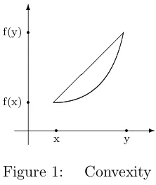
4.17 We use the fact that the graph of a convex function is convex, that is if x, y are real numbers with x < y then the straight-line segment joining the points (x, f(x)) and (y, f(y)) lies above or on the graph of f between x and y. (See Figure 1 below.)
6
-q q
x y
q q
[image:4.595.248.359.598.729.2]f(x) f(y)
Figure 1: Convexity
Any point on this straight-line segment is of the form
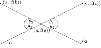
Now the graph of f at the point λx+(1−λ)y has height f(λx+ (1−λ)y) and the definition of convexity says that this height is not greater than λf(x) + (1−λ)f(y). For any point a∈R choose b < a and c > a, so a= λb+ (1−λ)c for some λ∈(0,1). Let L1 be the straight line through the points (a, f(a)) and (c, f(c))
and let L2 be the straight line through (b, f(b)) and (a, f(a)) (see Figure 2).
The idea of the proof is that by convexity the graph of f on [b, c] is trapped in the double cone formed by the lines L1, L2 and from this we can deduce continuity
of f at a.
H H
H H
H H
H H
H H
H H
H H
q
q(b, f(b)) (c, f(c))
q
(a, f(a))
L1 L2
θ1 θ2
θ3 θ4
[image:5.595.218.390.166.248.2]
Figure 2: Convex continuity
First, by convexity applied on [a, c] for any x ∈ (a, c) the point (x, f(x)) is below or on L1. Less obvious but also true is the fact that (x, f(x)) is above
or on L2. This follows from convexity applied between b and x : if (x, f(x))
were below L2 then (a, f(a)) would be above the straight-line segment joining
(b, f(b)) to (x, f(x)), contradicting convexity. By a similar argument we can show that if x∈(b, a) then the point (x, f(x)) lies below L2 and above L1.
Now to prove continuity at a, , let θ1, θ2, θ3, θ4 be the angles indicated in Figure
2. Given ε >0 choose a positive δ < ε/M where
M = max{|tanθ1|,|tanθ2|,|tanθ3|,|tanθ4|}.
Then for any x satisfying |x −a| < δ we have |f(x)−f(a)|6M δ and so
|f(x)−f(a)|< ε as required.
Chapter 5
5.1 From the triangle inequality d(x, z)6d(x, y)+d(y, z) so d(x, z)−d(y, z)6d(x, y). From the triangle inequality and symmetry d(y, z)6d(y, x) +d(x, z) =d(x, y) +d(x, z), so (y, z)−d(x, z)6d(x, y). Together these give |d(x, z)−d(y, z)|6d(x, y).
5.3 The proof is by induction on n. For n= 3 it is the triangle inequality. Suppose it is true for a given integer value of n>3. Then, using the triangle inequality and the inductive hypothesis we get that d(x1, xn+1) is less than or equal to
d(x1, xn) +d(xn, xn+1)6d(x1, x2) +d(x2, x3) +. . .+d(xn−1, xn) +d(xn, xn+1),
5.5 Suppose for a contradiction that z ∈ Bε(x)∩Bε(y). Then d(z, x)< ε and d(z, y)< ε, so by the triangle inequality and symmetry we get
d(x, y)6d(x, z) +d(z, y) =d(z, x) +d(z, y)<2ε.
This contradicts the fact that d(x, y) = 2ε.
5.7 Since S is bounded, we have for some (a1, a2, . . . , an)∈Rn and some K∈R
p
(x1−a1)2+ (x2−a2)2+. . .+ (xn−an)2 6K for all (x1, x2, . . . , xn)∈S.
In particular, for each i = 1,2, . . . , n, |xi−ai| 6 K so xi ∈ [ai −K, ai+K]. Let a=m−K and b=M+K where we define m= min{ai:i= 1,2, . . . , n}, and M = max{ai : i= 1,2, . . . , n}. Then xi ∈ [a, b] for each i = 1,2, . . . , n so (x1, x2, . . . , xn)∈[a, b]×[a, b]×. . .×[a, b] (product of n copies of [a, b] ).
This holds for all (x1, x2, . . . , xn) in S, so S ⊆[a, b]×[a, b]×. . .×[a, b] (product of n copies of [a, b] ).
5.9 Let the metric space be X. There exists some x0 ∈X and some K∈R such that d(b, x0) 6 K for all b ∈ B. Since A ⊆ B this holds in particular for all
points in A , so A is bounded.
If A=∅ then by definition diam A= 0 so diam A6 diam B, since the latter is the sup of a set of non-negative real numbers. Now suppose A 6= ∅. Since d(b, b0)6 diam B for all b, b0 ∈ B, in particular d(a, a0) 6 diam B for any a, a0 ∈A. Since diam A is the sup of such distances, diam A6 diam B.
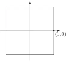
5.11 Since d∞((x, y),(0,0)) = max{|x|,|y|}, (x, y)∈Bd∞
1 ((0,0)) iff −1< x <1
and also −1< y <1, so the unit ball is the interior of the square shown in Figure 3 below.
6
-q
[image:6.595.238.350.466.580.2](1, 0)
Figure 3
5.13 Since any open ball is an open set by Proposition 5.31, any union of open balls is an open set by Proposition 5.41.
Conversely, given an open set in a metric space X, for each x∈U there exists by definition εx > 0 such that Bεx(x) ⊆ U. Then U =
[
x∈U
Bεx(x). For since each
Bεx(x) ⊆U, their union is contained in U. Also, any x ∈ U is in Bεx(x) and
hence is in the union on the right-hand side.
(b) If U is d-open then for any x∈U there exists ε >0 such that Bεd(x)⊆U. Then Bε/kd0 (x)⊆Bεd(x)⊆U. So U is d0-open.
(c) This follows from (b) together with Exercise 5.14.
5.17 Let x, y, z, t∈X. From Exercise 5.2,
|d(x, y)−d(z, t)|6d(x, z) +d(y, t) =d1((x, y),(z, t)).
So given ε >0 we may take δ =ε and if d1((x, y),(z, t))< δ then
|d(x, y)−d(z, t)|< δ=ε, so d:X×X→Ris continuous.
Chapter 6
6.1 (a) (i) The complement of [a, b] in R is (−∞, a)∪(b,∞), a union of open intervals which is therefore open in R. So [a, b] is closed in R.
(ii) The complement of (−∞,0] in R is (0,∞) which is open in R so (−∞,0] is closed in R.
(iii) The complement (−∞,0)∪(0,∞) is open in R so {0} is closed in R.
(iv) The complement is (−∞,0)∪(1,∞)∪ [
n∈N
(1/(n+ 1),1/n) which is open in
R so this set is closed in R.
(b) The complement of the closed unit disc in R2 is S={(x1, x2)∈R2 :x21+x22>1}.
If (x1, x2) ∈ S, let us put ε= p
x2
1+x22−1. Then Bε((x1, x2)) ⊆ S since if
(y1, y2) is in Bε((x1, x2)) then writing 0, x, y for (0,0),(x1, x2),(y1, y2)
re-spectively, we have from the reverse triangle inequality
d(0, y)>d(0, x)−d(x , y)> d(0, x)−ε=
q
x2
1+x22−ε= 1,
so y∈S. Hence S is open in R2 so the closed unit disc is closed in R2.
(c) Let S be the complement of this rectangle R in R2. Then S may be written as the union of the four sets
U1 =R×(−∞, c), U2 =R×(d, ∞), U3 = (−∞, a)×R, U4 = (b,∞)×R.
Each of these is open in R2. For example if (x1, x2) ∈ U1 then x2 < c. Take
ε=c−x2. We shall prove that Bε((x1, x2))⊆U1. For if (y1, y2) ∈Bε((x1, x2))
then |y2−x2|< ε=c−x2 so y2−x2< c−c2 which gives y2 < c so (y1, y2)∈U1
as claimed. This shows that U1 is open in R2. Similar arguments show that U2, U3, U4 are open in R2. Hence S =U1∪U2∪U3∪U4 is open in R2, and R is therefore closed in R2.
(d) In a discrete metric space X any subset of X is open in X ; in particular the complement in X of any set C is open in X so C is closed in X.
(e) It was proved on p.61 of the book that this subset is closed in C([0,1]).
in X. The union of a finite number of sets closed in X is also closed in X by Proposition 6.3, and the result follows.
6.5 Since Cn is the union of a finite number (namely 2n ) of closed intervals, Cn is closed in R for each n∈N so C is closed in R by Exercise 6.4.
6.7 We note first that {0,1} are points of closure of each of these intervals, since given any ε >0 there is a point of each of these intervals in Bε(i) for i= 1,2.
But also, if x6∈[0,1] then either x <0 or x >1, and in either case there exists ε >0 such that Bε(x)∩[0,1] =∅, so x is not a point of closure of [0,1]. This completes the proof.
6.9 Suppose that A is a non-empty subset of R which is bounded above and let u= sup A. Take any ε >0. Then by leastness of u there is some a∈ A with a > u−ε. Since u is an upper bound for A, also a6 u. So a∈ A∩Bε(u). this shows that u∈A. The proof for inf is similar.
6.11 The sets in Exercise 6.2 (a) and (d) are closed in R so by Proposition 6.11 (c) they are their own closures in R. The closure of the set in (b) is R: for given any x∈R and any ε >0 there exists an irrational number in (for example) (x−ε, x) by Exercise 4.8. The closure of the set A in 6.11(c) is A∪ {1} : for given any ε >0 there exists n∈N with 1/(n+ 1)< ε, which says that 1−n/(n+ 1)< ε, and this shows that 1∈A. Also, no point in the complement of A∪ {1} is in A: for the complement of A∪ {1} in R is
−∞, 1
2
∪(1,∞)∪
∞
[
n=1
n n+ 1,
n+ 1 n+ 2
, which is open in R.
The closure of the set in (d) is the set itself, since it is closed - its only limit point in R is 0.
6.13 First suppose that f :X→Y is continuous. Let y∈f(A) for some A⊆X and let ε >0. Then y =f(x) for at least one x∈A. By continuity of f at x there exists δ >0 such that f(Bδ(x))⊆Bε(y). By definition of A there exists some a∈A∩Bδ(x). Then f(a)∈f(Bδ(x))⊆Bε(y). So f(a) is in Bε(y)∩f(A) which shows that y∈f(A). Hence f(A)⊆f(A).
Conversely suppose that f(A) ⊆ f(A) for any subset A of X. We shall prove that the inverse image of any closed subset V of Y is closed in X , so that f is continuous by Proposition 6.6. For suppose that V is closed in Y. We have
f(f−1(V))⊆f(f−1(V), and f(f−1(V)⊆V sof(f−1(V)⊆V =V,
where the last equality follows from Proposition 6.11 (c) since V is closed in Y. Hence f(f−1(V) ⊆ V, so f−1(V) ⊆f−1(V). Since we always have the other
in-clusion f−1(V)⊆f−1(V), this shows that f−1(V) equals f−1(V), and f−1(V)
is closed in X by Proposition 6.11 (c).
6.15 Since for each i ∈I we have that Ai ⊆Ai, it follows that \ i∈I
Ai⊆\
But each Ai is closed in X by Proposition 6.11 (c) so \ i∈I
Ai is closed in X by
Proposition 6.4, and hence by Proposition 6.11 (f) \ i∈I
Ai ⊆
\
i∈I Ai.
In R we may take A1= (0,1), A2= (1,2). Then A1∩A2 =∅ so A1∩A2 =∅,
whereas A1 = [0,1] and A2 = [1,2] so A1∩A2 ={1}.
6.17 (a) Each point in A = [1,∞) is a limit point of A , since given any x ∈R with 1 6 x and any ε > 0, the open ball (x−ε, x+ε) contains points of A other than x (for example x+ε/2 ). Also, no point in the complement of A is a limit point of A , since any limit point of A is in A, and we have seen in Exercise 6.9 that A=A. So the set of limit points of A in R is precisely A.
(b) Any real number is a limit point of R\Q in R , since given x∈R and ε >0, by Exercise 4.8 there is an irrational number for example in (x−ε, x) and this is not equal to x. So the set of limit points here is R.
(c) We know from Definition 6.15 that any limit point of A in R is a point of closure of A, and we have seen in Exercise 6.9 that A =A∪ {1}. Now 1 is a limit point of A in R , since given any ε >0 there exists an n∈N such that 1/(n+ 1)< ε, so 1−ε < n/(n+ 1)<1, showing that 1 is a limit point.
But if x=n/(n+ 1) for some n∈N then we may take
ε= (n+ 1)/(n+ 2)−n/(n+ 1) = 1/(n+ 1)(n+ 2)
and then (x−ε, x+ε)∩A={n/(n+ 1)}, so x is not a limit point of A. The upshot is that the set of limit points here is the singleton {1}.
(d) The only limit point of the set in Exercise 6.2 (d) is 0.
6.19 Assume the result of Proposition 6.18, and first assume that the subset A is closed in X. Then A =A by Proposition 6.11 (c). By Proposition 6.18 all limit points of A are in A, hence in A.
Conversely suppose that the subset A⊆X contains all its limit point in X. Then by Proposition 6.18 A=A and A is closed in X by Proposition 6.11 (c).
6.21 (a) In each case we have already seen that the closure in R is [a, b] (this is the same as Example 6.8 (a)) so it is enough to show that the interior is (a, b). This follows from Proposition 6.21 (f) - the interior of a set A in X is the largest set contained in A and open in X.
(b) We have seen that the closure of Q in R is R. It is therefore enough to show that the interior of Q in R is ∅. But this is true, since given any x∈R and any open set U in R containing x, there is an ε >0 such that (x−ε, x+ε)⊆U. But any such open interval contains irrational numbers, so U cannot be contained in Q, so x is not in the interior of Q in R.
6.23 (a) By definition ∂A = A\A◦ , and A◦ ⊆ A ⊆ A so A◦ = A\∂A. Since
A◦ ⊆A, in fact A◦ =A\∂A.
x∈X\A⇔ any open set U 3x has non-empty intersection with X\A⇔ no
open set U 3x is contained in A⇔ x6∈A◦ ⇔x∈X\A◦ .
(c) By definition ∂A = A\A◦ . Now using Exercise 2.1 (with the C, D of that
exercise taken to be A◦ , A respectively) we have A\ A◦ = (X \ A◦ ) ∩A. So
∂A = (X\A◦ )∩A = X\A∩A, where the second equality uses (b) above. The second equality in the question follows by symmetry.
(d) This follows from (c), since ∂A is the intersection of the two closed sets X\A and A.
6.25 Let the metrics on X, Y be dX, dY. First suppose that f : X → Y is continuous. Let (xn) be a sequence in X converging to a point x0 ∈ X.
Then by continuity of f at x0, given ε > 0 there exists δ > 0 such that
dY(f(x), f(y)) < ε whenever dX(x, y) < δ. Since (xn) converges to x0 there
exists an integer N such that dX(xn, x0)< δ whenever n>N. So for n>N
we have dY(f(xn), f(x0))< ε. This proves that (f(xn)) converges to f(x0).
Conversely suppose that (f(xn)) converges to f(x0) whenever (xn) converges
to a point x0. We shall prove by contradiction that f is continuous at x0. For
if it is not, then for some ε >0 there is no δ >0 such that dY(f(x), f(y))< ε whenever dX(x, x0)< δ. In particular, for each n∈N there exists a point, call it xn, such that dX(x, y) <1/n yet dY(f(x), f(y))>ε. Now (xn) converges to x0 but (f(xn)) does not converge to f(x0). This contradiction proves that f is
continuous at x0, and the same applies at any point of X.
6.27 Since d(2)(x, y)6d(x, y) for all x, y∈X , we see that as in Exercise 5.15 (a), Bεd(x)⊆B(2)ε (x) for all x∈X and ε >0. Hence if U ⊆X is d(2) -open it is also d-open. Conversely suppose that U is d -open and let x∈U. Then Bdε(x)⊆U for some ε > 0, and we may take ε <1. Then Bεd(2)(x) =Bεd(x)⊆U, so U is d(2) -open. This shows that (X, d) and (X, d(2)) are topologically equivalent.
Since d(3)(x, y)6d(x, y) for all x, y∈X, as for d(2) when a subset U ⊆X is d(3) -open it is also d-open. Conversely suppose that U is d-open and x ∈U.
Then Bdε(x) ⊆ U for some ε > 0. Let δ = min{ε/2,1/2}. If d(3)(x, y) < δ then d(3)(x, y)<1/2, so
d(x, y) = d
(3)(x, y)
1−d(3)(x, y) 62d
(3)(x, y)< ε.
Then Bδd(3)(x) ⊆Bεd(x) ⊆U, so U is d(3) -open. This proves that (X, d) and (X, d(3)) are topologically equivalent.
Chapter 7
7.1 (a) Any topology on {0,1} has to contain ∅ and {0,1}. It may contain either, neither or both of {0} and {1} and each of these possibilities gives a topology. So there are precisely four distinct topologies on X = {0,1}, namely
(b) The combinatorics of the situation rapidly increase in complexity with the num-ber of points in X. If X={0,1,2} then again any topology on X must contain X and ∅, but there are now many topologies (29 in fact). One way to keep track of them is to list them by the number of singleton sets in them.
If there are no singleton sets in the topology, then the topology must have at most one set of order two in it (for if say {0,1} and {0,2} are in the topology then by the intersection property (T2) so is the singleton {0} : we get four topologies
{∅, X},{∅,{0,1}, X},{∅,{0,2}, X},{∅,{1,2}, X}.
If there is just one singleton set in the topology, and if it is {0}, then there are five possible topologies: these are {∅,{0}, X},{∅,{0},{0,1}, X},{∅,{0},{0,2}, X},
{∅,{0},{1,2}, X},{∅,{0},{0,1},{0,2}, X}.
There are five analagous topologies in which the only singleton is {1} and another five in which the only singleton is {2}.
Next we list the topologies with precisely two singleton sets in them. There are those with just one set of order two and those with two sets of order two in them. For example if the two singleton sets are {0},{1} then we get just one topology with precisely one set of order two, namely {∅,{0,},{1},{0,1}, X} . We get two topologies with these same singleton sets and precisly two sets of order two,
{∅,{0},{1},{0,1},{0,2}, X} and {∅,{0},{1},{0,1},{1,2}, X}. We also get three topologies in which the singletons are {0},{2} and three more in which the singletons are {1},{2} .
Finally, if the topology contains all three possible singletons, then it is the discrete topology (all subsets of X are in the topology). Altogether this gives 29 distinct topologies.
7.3 Suppose that T1,T2 are topologies on a set X. Then so is T1∩ T2. For (T1) ∅, X∈ T1 and ∅, X ∈ T2 so ∅, X∈ T1∩ T2.
(T2) If U, V ∈ T1∩ T2 then U, V ∈ T1 and T1 is a topology so U ∩V ∈ T1.
Similarly U ∩V ∈ T2 so U ∩V ∈ T1∩ T2.
(T3) If Ui ∈ T1∩ T2 for all i in some index set I , then for all i∈I, Ui ∈ T1
so [ i∈I
Ui ∈ T1 since T1 is a topology. Similarly [
i∈I
∈ T2 so [ i∈I
U1 ∈ T1∩ T2.
The union of the topologies {∅,{0},{0,1}} and {∅,{1},{0,1} is the discrete topology on {0,1}. But the union of the topologies {∅,{0}, X} and {∅,{1}, X}
on X = {0,1,2} is {∅,{0},{1}, X} which is not a topology on X since the union of {0},{1} is not in it.
We see that the argument above for the intersection of two topologies works exactly the same way for the intersection of any family of topologies.
7.5 Let T be defined on a set X as in Example 7.9.
(T1) By definition ∅ ∈ T. Also, since X\X=∅ is finite, X∈ T.
(T2) Suppose that U, V ∈ T. If either is empty, then so is U∩V so U∩V ∈ T. Otherwise X\U and X\V are both finite, hence X\(U∩V) = (X\U)∪(X\V) is also finite, so U∩V ∈ T.
(T3) Suppose that Ui ∈ T for all i in some index set I. If all the Ui are empty then so is [
i∈I
Ui and hence it is in T. Otherwise Ui0 6= ∅ for some i0 ∈ I, so
X\Ui0 is finite. Then X\
[
i∈I Ui
!
⊆X\Ui0 is also finite, so
[
i∈I
Chapter 8
8.1 (a) In this case the inverse image of any open set is itself hence it is open, so f is continuous.
(b) Let the constant value of f be y0 ∈ Y. Then f−1(U) =X if y0 ∈U and
f−1(U) =∅ if y06∈U. In either case f−1(U) is open so f is continuous.
(c) In this case f−1(U) is open in X for any subset U ⊆Y so f is continuous.
(d) The only open sets of Y are ∅, Y. Now f−1(∅) =∅ and f−1(Y) = X. So f is continuous since both ∅ and X are open in X.
8.3 Suppose first that A is open in X . The only open sets in S are ∅,S and
{1}. Now χ−A1(∅) =∅, χA−1(S) =X and χ−A1(1) =A, all of which are open in X so χA is continuous.
Conversely suppose that χA is continuous. Then A is open in X since A=χ−A1(1) and {1} is open in S.
8.5 We need to show that any open subset U ⊆R is a union of finite open intervals. By definition of the usual topology on R, for any x ∈ U there is some εx >0 such that (x−εx, x+εx)⊆U. It is straightforward to check that
U = [ x∈U
(x−εx, x+εx).
8.7 We have to show that B is a basis, and that it is countable. We first show that
B is a basis. For this we need to show that any open subset U ⊆R2 is the union
of a subfamily of B.
So let U be an open subset of R2 and let (x, y)∈U. It is enough to show that there is a set B ∈ B such that (x, y) ∈B ⊆U. First, there exists ε > 0 such that B3ε((x, y)) ⊆ U. Now choose a rational number q such that ε < q < 2ε.
Let q1, q2 be rational numbers with |x−q1|< ε/ √
2 and |y−q2|< ε/ √
2. Let us write d for the Euclidean distance in R2. Then
d((q1, q2),(x, y)) = p
(x−q1)2+ (y−q2)2< ε.
Hence (x, y)∈Bε((q1, q2))⊆Bq((q1, q2))∈ B. Also,
Bq((q1, q2))⊆B3ε((x, y))⊆U : for if (x0, y0)∈Bq(q1, q2) then
d((x0, y0),(x, y))6d((x0, y0),(q1, q1)) +d((q1, q2),(x, y))< q+ε <3ε.
This shows that U is a union of sets in B.
To show that B is countable, note that there is an injective function from B to Q3 defined by Bq((q1, q2))7→(q, q1, q2). Now B is countable by standard facts about
countable sets: Q is countable, a finite product of countable sets is countable, and any set from which there is an injective function to a countable set is countable.
9.1 The complement of any subset V of a discrete space X is open in X, so V is closed in X.
9.3 We may choose for example U = (0,1)∪(2,4), V = (1,3). Then
U∩V = (2,3], U∩V = [2,3), U∩V ={1} ∪[2,3], U∩V = [2,3].
9.5 (a) This is false in general. For a counterexample let X be the space {0,1}
with the discrete topology, let Y be the space {0,1} with the indiscrete topology, and let f be the identity function. Then f is continuous e.g. by Exercise 8.1 (c) or (d). Also, A ={0} is closed in X but f(A) =A is not closed in Y. (The analogous counterexample would work for any set with at least two points in it.)
(b) Again this is false: Exercise 9.3 gives a counterexample - take A= (0,1)∪(2,4) and B= (1,3) in R, and we have A∩B = (2,3] while A∩B = [2,3].
(c) This is also false. Let f be as in the counterexample to (a) and let B ={0}. Then the closure of B in Y is B ={0,1} so f−1(B) ={0,1} but f−1(B) ={0}
so the closure of this in X is f−1(B) ={0}.
9.7 Suppose first that f :X →Y is continuous and that A⊆X. Let y ∈f(A), say y=f(x) where x∈A. Let U be any open subset of Y containing y. Then f−1(U) is open in X and x∈f−1(U). Hence there exists a∈A∩f−1(U), and then f(a)∈U. Hence y∈f(A). This shows that f(A)⊆f(A).
Conversely suppose that f(A) ⊆ f(A) for any subset A ⊆ X. In particular we apply this when A=f−1(V) where V is closed in Y. Then
f(f−1(V)⊆f(f−1(V))⊆V =V.
Hence f−1(V) ⊆ f−1(V). Since f−1(V) ⊆ f−1(V) we have f−1(V) = f−1(V)
so by Proposition 9.10 (c) f−1(V) is closed in X, showing that f is continuous.
9.9 (a) If a ∈ A◦ then by definition there is some open set U of X such that
a∈U ⊂A. In particular then a∈A. So A◦ ⊆A.
(b) if A⊆B and x∈A◦ then by definition there is some open subset U of X
such that x∈U ⊆A. Since A⊆B then also U ⊆B, so x∈B◦ . This proves
that A◦ ⊆B◦ .
(c) If A is open in X then for every a∈ A there is an open set U (namely
U =A ) such that a∈U ⊆A, so a∈A◦ . This shows that A⊆A◦ and together
with (a) we get A=A◦ .
Conversely if A =A◦ then for every a∈A there exists an open set, call it Ua, such that a∈Ua ⊆A. It is straightforward to check that A=
[
a∈A
Ua which is a
union of sets open in X hence is open in X.
point x∈U we have x∈U ⊆A, so also x ∈A◦ . This shows that a∈U ⊆A◦ ,
and U is open in X, so a is in the interior of A◦ . These together show that
the interior of A◦ is A◦ .
(e) This follows from (c) and (d).
(f) We know that A◦ is open in X from (e). Suppose that B is open in X and
that B⊆A. By (b) then B◦ ⊆A◦ . Since B is open we have B◦ =B by (c). So
B ⊆A◦ , which says that A◦ is the largest open subset of X contained in A.
9.11 Since Ai
◦
⊆ Ai for each i = 1,2, . . . , m we get m
\
i=1
Ai
◦ ⊆
m
\
i=1
Ai. Also,
m
\
i=1
Ai
◦
is the intersection of a finite family of open sets hence is open in X,
hence it is contained in the interior of m
\
i=1
Ai. Conversely m
\
i=1
Ai ⊆Aj for each
j= 1,2, . . . , m; it follows (9.9 (b)) that the interior of m
\
i=1
Ai is contained in Aj
◦
for each j= 1,2, . . . , m, so the interior of m
\
i=1
Ai is contained in m
\
i=1
Ai
◦
. This
proves the result.
9.13 This follows from the fact that ∂A=A∩X\A (Proposition 9.20) since each of A, X\A is closed in X hence so is their intersection.
9.15 Since ∂A=A\A◦ , we have ∂A∩A◦ =∅. By the definition ∂A=A\A◦
we know that ∂A ⊆ A and A◦ ⊆ A ⊆ A. So the disjoint union ∂AtA ⊆ A.
Conversely since ∂A= A\A◦ , we have A ⊆A◦ t∂A. These two together show
that A=A◦ t∂A.
Now if B ⊆ X and B ∩A 6= ∅ then B ∩A 6= ∅ so either B ∩A◦ 6= ∅ or B∩∂A6=∅.
Chapter 10
10.1 The subspace topology TA consists of all sets U ∩A where U ∈ T. Hence
TA={∅,{a}, A}.
A. Either V =∅ and then V = A∩ ∅ ∈ TA, or A\V is finite. In this latter case let U = (X\A)∪V. Then A∩U =V, and U is in the co-finite topology for X since X\U =A\V and the latter is finite.
Conversely suppose that V =A∩U where U is in the co-finite topology T for X. Then either U =∅, so V =A∩U =∅, and V is in the co-finite topology for A , or else X\U is finite, in which case A\V ⊆X\U is finite and again V is in the co-finite topology for A.
10.5 Since V is closed in X its complement X\V is open in X. Now we have A\(V ∩A) =A∩(X\V) by Exercise 2.2. So A\(V ∩A)∈ TA. This shows that V ∩A is closed in (A,TA).
10.7 (a) We use Proposition 3.13: for any subset B ⊆Y we have
f−1(B) =[ i∈I
(f|Ui)−1(B).
Now let B be open in Y. For each i ∈ I continuity of f|Ui implies that (f|Ui)−1(B) is open in Ui and hence, by Exercise 10.6 (a), open in X. Hence f−1(B) is a union of sets open in X , so f−1(B) is open in X. Thus f is continuous as required.
(b) We again use Proposition 3.13: for any subset B ⊆Y we have
f−1(B) =[ i∈I
(f|Vi)−1(B).
Now suppose that B is closed in Y. Then continuity of f|Vi ensures that (f|Vi)−1(B) is closed in V , and hence, by Exercise 10.6 (b) it is closed in X. Hence f−1(B) is the union of a finite number of sets closed in X, so f−1(B) is closed in X, and f is continuous as required.
10.9 (a) First suppose x ∈B1. Then x ∈X1 and also for any set W open in
X1 with x ∈W we have W ∩A6=∅. Now let U be any set open in X2 with
x∈U. Then W =U∩X1 is open in X1 and contains x, so W ∩A6=∅. Then
U∩A=U∩(A∩X1) = (U∩X1)∩A=W ∩A6=∅, so x∈B2. Since also x∈X1
this shows that B1⊆B2∩X1.
Conversely suppose that x∈B2∩X1. Then x∈X1 and for any subset U open
in X2 we know U∩A6=∅. Now let W be an open subset of X1 with x∈W.
Then W =X1∩U for some U open in X2 with x∈U. Hence U∩A6=∅, so
since A⊆X1 we have U ∩A =U ∩X1∩A=W ∩A, so W ∩A6=∅ , showing
that x∈B1.
Taking these two together, we have B1=B2∩X1.
10.11 Any singleton set {(x, y)} in X×Y is the product {x}×{y} of sets which are open in X, Y since they have the discrete topology so {(x, y)} is open in the product topology. Hence any subset of X×Y is open in the product topology, which is therefore discrete.
complement of U×Y is (X\U)×Y, which is infinite. So U×Y is not open in the co-finite topology on X×Y although it is open in the product of the co-finite topologies on X and Y.
10.15 (a) Any open subset W of X×Y is a union [ i∈I
Ui×Vi for some index
set I , where each Ui is open in X and each Vi is open in Y. We may as well assume that no Vi (and no Ui ) is empty, since if it were then Ui ×Vi would be empty, and hence does not contribute to the union. The point of this is that pX(Ui×Vi) =Ui for all i∈I. Now
pX(W) =pX
[
i∈I
Ui×Vi
!
=[ i∈I
pX(Ui×Vi) =
[
i∈I Ui,
which is open in X as a union of open sets. Similarly pY(W) is open in Y.
(b) Consider the set W ={(x, y)∈R2:xy= 1} . This is closed in
R2: a painless way to see this is to consider the function m:R×R→R given by m(x, y) =xy. Since m is continuous by Propositions 8.3 and 5.17, and {1} is closed in R, W =m−1(1) is closed in R×R by Proposition 9.5. But p1(W) =R\ {0} is not closed in R.
10.17 Since t is clearly one-one onto, it is enough to prove that t and t−1 are continuous. Now t is continuous by Proposition 10.11, since if p1, p2 are the
projections of X×X on the first, second factors, then p1◦t=p2 and p2◦t=p1
and p1, p2 are both continuous. Now we observe that t is self-inverse, i.e. t−1=t
so t is a homeomorphism.
10.19 (a) The graph of f is a curve through the point (0,1) which has the lines x =−1, x= 1 as asymptotes. We argue as in the proof of Proposition 10.18: let θ:X → Gf be defined by θ(x) = (x, f(x)) and let φ:Gf → X be defined by φ(x, f(x)) =x. Then θ and φ are easily seen to be mutually inverse. Continuity of θ follows from Proposition 10.11, since p1◦θ is the identity map of X and p2◦θ
is the continuous function f. Continuity of φ follows since φ is the restriction to Gf of the continuous projection p1 :X×R→X. Hence θ is a homeomorphism (with inverse φ).
(b) The graph of f is not easy to draw, but it oscillates up and down with decreasing amplitude as x approaches 0 from the right. The continuity of f : [0,∞) → R on (0,∞) follows from continuity of the sine function together with Propositions 8.3 and 5.17. Continuity (from the right) at 0 follows from Exercise 4.14. Now arguing as in Proposition 10.18 we see that x7→(x, f(x)) defines a homeomorphism from [0,∞) to Gf.
Chapter 11
11.3 We can prove this by induction on n. When n= 2 the conclusion is simply the Hausdorff condition. Suppose the result is true for a given integer n with n>2 and let x1, x2, . . . , xn+1 be distinct points of X. By inductive hypothesis,
for i= 1,2, . . . , n there exist pairwise disjoint open sets Wi with xi ∈Wi. Also, by the Hausdorff condtion, for each i= 1,2, . . . , n there exist disjoint open sets Si, Ti such that xi ∈Si, xn+1∈Ti. For each i= 1,2, . . . , n put Ui =Si∩Wi,
and put Un+1=
n
\
i=1
Ti. Then U1, U2, . . . , Un are disjoint since W1, W2, . . . , Wn
are, and for each i = 1,2, . . . , n we have Ui ∩Un+1 = ∅ since Ui ⊆ Si and Un+1⊆Ti. Also, by construction each of U1, U2, . . . Un, Un+1 is open in X. Thus
U1, U2, . . . , Un+1 are pairwise disjoint open sets. This completes the inductive step.
11.5 We prove that (X×Y)\Gf is open in X×Y. (Once we have opted for this, the rest of the proof ‘follows its nose’.) It is enough, by Proposition 7.2, to show that for every point (x, y) ∈ (X×Y)\Gf there exists an open subset W of X×Y with (x, y)∈W ⊆(X×Y)\Gf. So let (x, y)∈(X×Y)\Gf. Then (x, y) 6∈ Gf so f(x) 6= y. Since Y is Hausdorff there exist disjoint open sets V1, V of Y such that f(x)∈V1, y∈V. Since f is continuous, U =f−1(V1) is
open in X. Note that x∈U since f(x)∈V1. Also, y∈V. Write W =U×V.
Then (x, y) ∈U ×V =W, and W ⊆(X×Y)\Gf since if (x0, y0) ∈W then x0 ∈ U and y0 ∈V so f(x0) ∈V1 and y0 ∈V, but V1∩V =∅ so f(x0)6=y0,
which says that (x0, y0)6∈Gf.
11.7 (a) Suppose first that X is a Hausdorff space. We shall prove that (X×X)\∆ is open in X×X from which it will follow that ∆ is closed in X ×X. (This proof is almost identical to that in Exercise 11.5.) So let (x, y)∈(X×X)\∆. By Proposition 7.2 it is enough to show that there is an open set W of X×X with (x, y) ∈ W ⊆ (X ×X)\∆. Since (x, y) ∈ (X×X)\∆ we have (x, y) 6∈ ∆, so y 6= x. Since X is Hausdorff there exist disjoint open subsets U, V of X such that x ∈ U, y ∈ V. Then W = U ×V is an open subset of X ×X, and (x, y) ∈ U ×V. Moreover W ⊆ (X ×X)\∆ since if (x0, y0) ∈ W then x0 ∈U, y0 ∈V and U ∩V =∅ so y0 6=x0, which says (x0, y0)6∈∆.
Conversely suppose that ∆ is closed in X×X. Then (X×X)\∆ is open in X×X. Let x, y be distinct points of X. Then y 6=x so (x, y) 6∈∆. Hence (x, y) is in the open set (X×X)\∆ and by definition of the product topology there exist open sets U, V of X such that (x, y)∈U ×V ⊆(X×X)\∆. Now x∈U, y∈V and U∩V =∅ since if z∈U∩V then (z, z)∈∆∩(U∩V) =∅. So X is Hausdorff.
(b) Consider the characteristic function χA:X×X→S of the set A= (X×X)\∆. Since χ−A1(∅) =∅, χ−A1(1) =A and χ−A1S=X×X we have that χA is continuous iff A= (X×X)\∆ is open in X×X, i.e. iff ∆ is closed in X×X, and by (a) this holds iff X is Hausdorff.
and g−1(0,∞) are clearly disjoint (if x ∈ g−1(−∞,0) then g(x) <0, while if x∈g−1(0,∞) then g(x)>0. ).
Chapter 12
12.1 (i) has the partition {B1((1,0)), B1((−1,0))} so it is not connected, hence
not path-connected. The others are all path-connected and hence connected. We can see this for (ii) and (iii) by observing that any point in B1((1,0)) may be connected
by a straight-line segment to the centre (1,0) (and this segment lies entirely in B1((1,0)) ), any point in X =B1((−1,0)) or B1((−1,0)) can be connected by a
straight-line segment in X (or in B1((−1,0)) ) to the centre (−1,0). Moreover
the points (1,0) and (−1,0) can be connected by straight-line segment which lies entirely in B1((−1,0))∪B1((1,0)), hence certainly in B1((−1,0))∪B1((1,0)).
To see that (iv) is path-connected note that any point (q, y) ∈ Q×[0,1] can be connected by a straight-line segment within Q×[0,1] to the point (q, 1) and that any two points in the line R× {1} can be connected by a straight-line segment entirely within this line.
Finally to see that the set S in (v) is path-connected, it is enough to show that any point (x, y) ∈S can be connected to the origin (0,0) by a path in S . If x ∈ Q we first connect (x, y) to (x,0) by a vertical line-segment in S , then we connect (x, 0) to (0,0) by a (horizontal) line-segment in S. If x6∈Q then y∈Q and we first connect (x, y) to (0, y) by a straight-line segment in S and then we connect (0, y) to (0,0) by a (vertical) straight-line segment in S.
12.3 Suppose that X is an infinite set with the co-finite topology and let U, V be non-empty open sets in X . The X \U and X\V are both finite, hence X\(U ∩V) = (X\U)∪(X\V) is finite. This shows that U∩V is nonempty -indeed it is infinite. Hence there is no partition of X, so X is connected.
12.5 We may prove that this is true for any finite integer n by induction. The result is certainly true when n= 1 and if it holds for a given integer n then for n+ 1 it follows from Proposition 12.16 applied to the connected sets A1∪A2∪. . .∪An (which is connected by inductive hypothesis) and An+1 : these have non-empty
intersection since An∩An+16=∅.
The analogous result is also true for an infinite sequence (Ai) of connected sets such that Ai∩Ai+1 6=∅ for each positive integer i . For suppose that {U, V} were
a partition of ∞
[
i=1
Ai. For each i∈ N we have either Ai ⊆U or Ai ⊆V, since
otherwise {U∩Ai, V ∩Ai} would be a partition of Ai. Let IU be the subset of all i∈ N for which Ai ⊆ U and let IV be the analogous set for V. Suppose w.l.o.g. that 1 ∈IU (otherwise switch the names of U and V ). Now n ∈ IU implies n+ 1 ∈ IU, for if An ⊆ U then the connected set An∪An+1 is also
contained in U, otherwise {(An∪An+1)∩U,(An∪An+1)∩V} would partition
An∪An+1. It follows that N⊆IU, so ∞
[
i=1
Ai ⊆U , contradicting the assumption
12.7 This follows from the intermediate value theorem since we may show that if the polynomial function is written f, then f(x) takes a different sign for x large and negative from its sign for x large and positive, so its graph must cross the x -axis somewhere. Explicitly, we may as well assume that the polynomial is monic (has leading coefficient 1)
f(x) =xn+an−1xn−1+. . .+a1x+a0 =xn+g(x),say.
Since g(x)/xn → 0 as x → ±∞, there exists ∆ ∈R such that |g(x)/xn| <1 for |x|>∆. This says that for large |x|, we have that f(x) and xn have the same sign. But n is odd, so f(x) <0 for x large and negative, and f(x)>0 for x large and positive.
12.9 Define g as the hint suggests. Then g is continuous on [0,1] and
g(0) +g(1/n) +. . .+g((n−1)/n) =f(0)−f(1/n) +f(1/n) +. . .+f((n−1)/n)−f(1)
=f(0)−f(1) = 0.
Hence we have only the following two cases to consider.
Case 1. All the g(i/n) are zero. Now if g(i/n) = 0 then f(i/n) =f((i+ 1)/n) and the conclusion holds with x=i/n.
Case 2, For some i= 0,1, . . .(n−1) the values g(i/n), g((i+ 1)/n have opposite signs. Then by the intermediate value theorem there exists some x∈(i/n, (i+1)/n) with g(x) = 0, so f(x) =f(x+ 1/n).
12.11 (a) This is false. For example let X=Y =R and A=B={0}. Then
X\A=Y \B =R\ {0}
which is not connected, but X×Y\(A×B) =R2\{(0,0)} which is path-connected and hence connected.
Note that common sense suggests (b) false (c) true, since the conclusion is the same for both, but the hypotheses are stronger in (c). (This proves nothing, but it is suggestive.)
(b) This is false. For example let X =R and let A= {0,1}, B = (0,1]. Then both of A∩B={1} and A∪B = [0,1] are connected, but A is not connected.
(c) This is true. We prove it in the style of Definition 12.1. So let f :A→ {0,1} be continuous, where {0,1} has the discrete topology. Then f|A∩B is continuous, and since A∩B is connected, f|A∩B is constant, say with value c (where c= 0 or 1 ). Define g:A∪B → {0,1} by g|A=f, g|B =c. Then g is continuous by Exercise !0.7 (b), since each of A, B is closed in X and hence in A∪B, and on the intersection A∩B the two definitions agree. But A∪B is connected, so g is constant. In particular this implies that f :A→ {0,1} is constant, so X is connected. Similarly B is connected.
12.13 Let y1, y2 ∈ Y. Since f is onto, f(x1) = y1, f(x2) = y2 for some
x1, x2∈X. Let g : [0,1] → X be a continuous path in X from x1 to x2.
Then f ◦g : [0,1] → Y is a continuous path in Y from y1 to y2. So Y is
path-connected.
6
=X ) non-empty subset of X is open and closed in X , it is connecetd iff every proper non-empty subset of X has non-empty boundary.
12.17 Suppose that f :A∪B → {0,1} is continuous, where {0,1} has the discrete topology. Since A and B are connected, both f|A and f|B are constant, say with values cA and cB in {0,1}. Let a ∈A∩B. Then f−1(cA) is an open set containing a and hence some point b ∈ B. But then f(b) = cA and also f(b) = cB since b ∈ B. So cA = cB, and f is constant. Hence A∪B is connected.
12.19 The idea of this example is an infinite ladder where we kick away a rung at a time. Explicitly, let
Vn= ([0,∞)× {0,1})∪
[
i∈N, i>n
{i} ×[0,1].
Then it is clear that each Vn is path-connecetd hence connected and that Vn⊇Vn+1
for each n∈N. But
∞
\
n=1
Vn= [0∞)× {0,1}, which is not connected.
Chapter 13
13.1 Suppose that the space X has the indiscrete topology. Then the only open sets in X are ∅, X. So any open cover of X must contain the set X, and {X}
is a finite subcover.
13.3 Suppose that U is an open cover of A∪B. In particular U is an open cover of A, so there is a finite subfamily UA of U which covers A. Similarly there is a finite subfamily UB of U which covers B. Then UA∪ UB is a finite subcover of U which covers A∪B and this proves that A∪B is compact.
13.5 Suppose that U is any open cover of (X, T). Since T ⊆ T0, each set in U
is in T0, hence U is an open cover of (X, T0) as well. But (X,T0) is compact, so there is a finite subcover. This proves that (X, T) is compact.
13.7 This is immediate since any finite subset of a space is compact.
13.9 Suppose first that X ⊆ R is unbounded. Let us define f : X → R by f(x) = 1/(1 +|x|). Then the lower bound of f is 0, since f(x) > 0 for all x ∈ X, but for any δ > 0 there exists x ∈ X such that 1 +|x| > 1/δ, and then f(x)< δ. But f does not attain its lower bound 0 since f(x)>0 for all x∈X.
δ >0 there exists x∈X with |x−c|< δ. But this lower bound is not attained since f(x)>0 for all x∈X.
13.11 This follows from Exercise 13.6 since the family {Vn :n∈N} has the finite intersection property - the intersection of any finite subfamily {Vn1, Vn2, . . . , Vnr}
is VN where N = max{n1, n2, . . . , nr} and VN 6=∅. Hence since X is compact,
Exercise 13.6 says that ∞
\
n=1
Vn is non-empty.
13.13 (a) We show that the Xn form a nested sequence of closed subsets of X. Note that X1 = f(X0) = f(X) ⊆ X0. Suppose inductively that Xn ⊆ Xn−1
for some integer n > 1. Then f(Xn) ⊆ f(Xn−1) which says Xn+1 ⊆ Xn. So
by induction Xn ⊆ Xn−1 for all n ∈ N. Also, since X is compact and f is continuous, X1 = f(X) is compact by Proposition 13.15. Suppose that Xn is compact for some integer n>0. Then since f is continuous, Xn+1 =f(Xn) is
also compact by Proposition 13.15. By induction Xn is compact for all integers n > 0. But X is Hausdorff, so each Xn is closed in X. Also, each Xn is
non-empty by inductive construction. Now by Exercise 13.11, A= ∞
\
n=0
Xn is
non-empty.
(b) The inclusion f(A) ⊆ A is straightforward: if a ∈ A then a ∈ Xn for any integer n > 0, so f(a) ∈f(Xn) =Xn+1 for any integer n > 0. But since
X0 ⊇ X1 ⊇ . . . ⊆Xn ⊇. . . , we have ∞
\
n=0
Xn+1 =
∞
\
n=1
Xn= ∞
\
n=0
Xn =A, and we
see that f(a)∈A.
To prove the other inclusion we follow the hint: for any a∈A let Vn=f−1(a)∩Xn. Since the Xn are nested so are the Vn. Since X is Hausdorff, {a} is closed in A, hence since f is continuous, f−1(a) is closed in X by Proposition 9.5. Also each Xn is closed in X as in (a). So each Vn is closed in X. Moreover, for each integer n > 0 we know a ∈ Xn+1 = f(Xn) so there exists x ∈ Xn such that f(x) = a. This says that Vn = f−1(a)∩Xn 6= ∅. Now by Exercise 13.11,
∞
\
n=0
Vn is non-empty. Let b be a point in this set. Then b ∈ Vn =f−1(a)∩Xn
for any integer n>0. Also, b=f−1(a) says that f(b) =a, and b∈Xn for all
integers n > 0 says that b∈
∞
\
n=0
Xn=A. So A ⊆ f(A). We have now proved
that f(A) =A.
13.15 The exercise gives the procedure for constructing the sequences (an), (bn). The sequence (an) converges to some real number c since it is monotonic increas-ing and bounded above (for example by b1 ). Likewise since (bn) is monotonic decreasing and bounded below (for example by a1 ) it too converges to some real
13.17 Suppose that T1, T2 are topologies on a set X such that T1 ⊆ T2, and that (X, T1) is Hausdorff and (X, T2) is compact. Consider the identity function from
(X, T2) to (X, T1). This is continuous since T1 ⊆ T2, and it is one-one onto. Since
(X, T1) is Hausdorff and (X, T2) is compact it follows from the inverse function theorem Proposition 13.26 that the identity function from (X, T2) to (X, T1) is
a homeomorphism, i.e. the identity function from (X, T1) to (X, T2) is also
continuous. This says that T2⊆ T1. So T1 =T2 as required.
In particular if X = [0,1] and T1 is a Hausdorff topology on [0,1] which is
contained in the Euclidean topology T2, then since we know that ([0,1],T2) is
compact, the first part of this exercise shows that T1 =T2. So T1 is not strictly coarser than the Euclidean topology T2.
13.19 Let X be a compact Hausdorff space, let W ⊆X be closed in X and let y∈X\W. Since W is a closed subspace of a compact space, W is compact by Proposition 13.20. For any w∈W, by the Hausdorff condition there exist disjoint open subsets Uw, Vw of X such that y ∈Uw, w ∈Vw. Now {Vw :w∈W} is an open cover of compact W , so there is a finite subcover {Vw1, Vw2, . . . , Vwr}.
Put
U = r
\
i=1
Uwi, V =
r
[
i=1
Vwi.
Then U, V are open in X. Also, W ⊆V since {Vw1, Vw2, . . . , Vwr} covers W.
Next, y ∈ U since y ∈ Uwi for all i ∈ {1,2, . . . , r}. Finally U and V are
disjoint, since for any point v ∈ V we have v ∈Vwi for some i ∈ {1,2, . . . , r}
so since Uwi and Vwi are disjoint, v6∈Uwi hence v 6∈U. This proves that X
is regular.
The proof that X is normal is similar. Suppose that W, Y are disjoint closed subsets of X. From the first part of this exercise, for each y ∈ Y there exist disjoint open subsets Uy, Vy of X such that y ∈Uy, W ⊆Vy. Now {Uy :y∈Y} is an open cover of Y, and Y is compact by Proposition 13.20, so there is a finite subcover {Uy1, Uy2, . . . , Uys}. Put
U = s
[
j=1
Uyj, V =
s
\
j=1
Vyj.
Then U, V are open in X. Also, Y ⊆U since {Uy1, Uy2, . . . , Uys} is a cover for
Y. Next, W ⊆V since W ⊆Vyj for all j ∈ {1,2, . . . , s}. Finally U and V
are disjoint, since if u∈U then u ∈Uyj for some j ∈ {1,2, . . . , s} so u6∈Vyj
since Uyj and Vyj are disjoint, so u6∈V. Hence X is normal.
13.21 First, following the hint we prove that
f−1(V) =pX(Gf ∩p−Y1(V)) for any subset V ⊆Y .
For if x ∈f−1(V) then f(x)∈V, and x=pX(x, f(x)) where (x, f(x))∈ Gf and also (x, f(x))∈p−Y1(V) since pY(x, f(x)) =f(x)∈V.
Suppose x∈pX(Gf∩p−Y1(V)). There exists y∈Y such that (x, y)∈Gf∩p1Y(V). Now (x, y)∈Gf says that y=f(x) and (x, y)∈p−Y1(V) says that y ∈V, so f(x)∈V so x∈f−1(V) as required.
9.5 since V is closed in Y. So Gf∩pY−1(V) is closed in X×Y and since Y is compact, by Exercise 13.20 (a) pX(Gf∩p−Y1(V)) is closed in X. This tells us that f−1(V), which equals pX(Gf ∩p−Y1(V)), is closed in X whenever V is closed in Y , so f is continuous by Proposition 9.5.
Chapter 14
14.1 Consider the sequence (1/n) in (0,1). This has no subsequence converging to a point of (0,1) since the sequence (1/n), and hence every subsequence of it, converges in R to 0.
14.3 Let A be a closed subset of a sequentially compact metric space X. Let (xn) be any sequence in A. Then (xn) is also a sequence in X, which is sequentially compact, hence there is a convergent subsequence (xnr). The point this converges
to must lie in A since A is closed in X (see Corollary 6.30). Hence A too is sequentially compact.
14.5 Let (yn) be a sequence in f(X). For each n∈N there is a point xn∈X such that yn=f(xn). Since X is sequentially compact there is some subsequence (xnr) of (xn) which converges to a point x ∈X. Then by continuity of f the
subsequence (ynr) = (f(xnr)) converges in Y to f(x) (see Exercise 6.25). Hence
f(X) is sequentially compact.
14.7 This follows from Exercises 14.5 and 14.2. For if f :X →Y is a continuous map of metric spaces and X is sequentially compact, then by Exercise 14.5 so is f(X), and hence by Exercise 14.2 f(X) is bounded.
14.9 Suppose that (X, dX) and (Y, dY) are sequentially compact metric spaces. In X×Y we shall use the product metric d1 : recall that
d1((x, y),(x0, y0)) =dX(x, x0) +dY(y, y0).
Let ((xn, yn)) be any sequence in X×Y. First, since X is sequentially com-pact there is a subsequence (xnr) of (xn) converging to a point x ∈ X. Now
consider the sequence (ynr) in Y. Since Y is sequentially compact there
ex-ists a subsequence (ynrs) of (ynr) converging to a point y in Y. Then (xnrs)
is a subsequence of (xnr) hence also converges to x. Consider the subsequence
((xnrs, ynrs)) of ((xn, yn)). This converges to (x, y). For let ε >0. Since (xnrs) converges to x, there exists S1 ∈ N such that dX(xnrs, x) < ε/2 whenever
s > S1. Similarly there exists S2 ∈ N such that dY(ynrs, y) < ε/2 whenever
s>S2. Put S = max{S1, S2}. If s>S then
d1((xnrs, ynrs),(x, y)) =dX(xnrs, x) +dY(ynrs, y) < ε.
14.11 Let xn ∈ Vn for each n ∈ N. Since X is sequentially compact, there is a subsequence (xnr) of (xn) converging to some point in X. Since the Vn are
nested, xnr ∈ Vm for all r such that nr > m. But Vm is closed in X, so
x ∈ Vm (by Corollary 6.30). This holds for all m ∈ N so x∈ ∞
\
n=1
Vn and this
intersection is non-empty.
14.13 The exercise does most of this! As suggested, we prove inductively that [a, ai] ⊆ A for a1, a2, . . . , an = b. This is true for i = 1 since a0 = a ∈ A,
and since a1−a0 < ε where ε is a Lebesgue number for the cover {A, B}, we
know that [a0, a1] is contained in a single set of the cover, and this must be A since
A∩B =∅. Suppose inductively that [a, ai] ⊆ A for some i ∈ {1,2, . . . n−1}. We can repeat the above argument with a replaced by an−1 and deduce that also
[an−1, an] ⊆ A. Hence [a, b]⊆ A, so {A, B} is not a partition of [a, b] after all. So [a, b] is connected.
14.15 If, say, Vn0 is empty, then ∞
\
n=1
Vn=∅ and its diameter is 0 by definition.
Likewise in this case diam Vn0 = 0 so
inf{diamVn:n∈N}= 0 also.
Suppose now that all the Vn are non-empty. (We already know from Exercise 14.11
that their intersection is then non-empty.) Now ∞
\
n=1
Vn⊆Vm for any m ∈ N so
diam ∞
\
n=1
Vn
!
6 diam Vm. Hence
diam ∞
\
n+1
Vn
!
6inf{diamVm :m∈N}=m0 say.
Conversely m0 is a lower bound for the diameters of the Vn so for any ε >0 and any n∈N we know that diam Vn> m0−ε. Hence there exist points xn, yn∈Vn
such that d(xm, xn)> m0−ε. Since X is sequentially compact (xn) has a
sub-sequence (xnr) converging to a point x∈X, and then (ynr) has a subsequence
(ynrs) converging to a point y ∈ X. Since (xnrs) is a subsequence of (xnr) it
too converges to x. Also, by continuity of the metric, d(xnrs, ynrs) →d(x, y) as s→ ∞. Hence d(x, y)>m0−ε. Also, x, y ∈Vn for each n∈N since Vn is
closed in X. Since this is true for all n∈N we have x, y∈
∞
\
n=1
Vn. Hence diam
∞
\
n=1
Vn>m0−ε. But this is true for any ε >0 , so diam
∞
\
n=1
Vn>m0.
The above taken together prove the result.
14.17 (a) Let x ∈ X. We want to show that x ∈ f(X). Consider the sequence (xn) in X defined by
Since X is sequentially compact there is a convergent subsequence, say (xnr).
Any convergent sequence is Cauchy, so given ε >0 there exists R∈N such that
|xnr −xns|< ε whenever s > r>R. Now we use the isometry condition, iterated
nR−1 times, to see that |x1−xnr−nR+1|< ε whenever r >R. But x1 =x and
xnr−nR+1∈f(X) whenever r > R. Hence x∈f(X). But X is compact and f
is continuous, so f(X) is compact. Also, X is metric so Hausdorff, hence f(X) is closed in X. Hence f(X) = f(X). So x∈f(X) for any x∈X , which says that f is onto. Hence f is an isometry.
(b) We can apply (a) to the compositions g◦f :X→ X and f ◦g:X → X to see that these are both onto. Since g◦f is onto, g is onto. Similarly since f ◦g is onto, f is onto. Hence both f and g are isometries.
(c) We define f : (0,∞)→(0,∞) by f(x) =x+ 1.
Chapter 15
15.1 (a) A figure-of-eight.
(b) A two-dimensional sphere. (See below.)
a
c
@ @ R
@
@b
---
x
@ @ R
@ @
z --- y
(c) This gives a M¨obius band. (See below.) For we first cut along the dashed vertical line in the triangle abc to get two triangles as in the middle picture, with vertical sides labelled to recall how these are to be stuck together. Then we reassemble these middle triangles to get the picture on the right, which represents a M¨obius band.
@
@ R
@ @
a
c b 66 66
@ @ R
@
@ 6
6 ? ?
15.3 It is clear that (0, t) ∼ (1,1−t) for any t ∈ [0,1], by (iv). What needs proving is that the equivalence classes are no bigger than the sets described in the question.
First if 0< s <1 and (s2, t2)∼(s, t) then (i) must apply and (s2, t2) = (s, t).
So (s, t) cannot be equivalent to any point other than itself - {(s, t)} is a complete equivalence class.
Consider now what points can be equivalent to (0, t), for some t ∈ [0,1]. So suppose that (s2, t2)∼(0, t). Then either(i) applies and (s2, t2) = (0, t) or (ii)
applies and s2= 1 and t2 = 1−t. Thus the set {(0, t), (1,1−t)} is a complete
equivalence class.
15.5 For example since [0, π) = (−∞, π)∩[0,2π] it follows that [0, π) is open in [0,2π]. Now f([0, π)) is the upper semi-circle of S1, closed at the end with co-ordinates (1,0) and open at the end (−1,0). This is not open in S1, since any open set in S1 containing the point (1,0) also contains points (x, y) ∈ S1 with y <0, and such points are not in f([0, π)).
15.7 This is proved by complements. By Proposition 3.9, X\f−1(V) =f−1(Y\V) for any subset V ⊆Y. Suppose that f :X →Y is a quotient map. Then V ⊆Y is closed in Y iff Y\V is open in Y, which happens iff X\f−1(V) =f−1(Y\V)
is open in X iff f−1(V) is closed in X.
Conversely suppose that V ⊆Y is closed in Y iff f−1(V) is closed in X. Then U ⊆Y is open in Y iff Y \U is closed in Y iff X\f−1(U) = f−1(Y \U) is closed in X iff f−1(U) is open in X, so f is a quotient map.
15.9 We proceed in the same way as in the proof that the quotient space of the square S= [0,2π]×[0,2π] by an appropriate equivalence relation is homeomorphic to T. Define
f :R2 →T by f((s, t)) = ((a+rcost) coss,(a+rcost) sins, rsint).
Then as in the proof mentioned above, we show that (a) f is a map to T,
(b) i◦f :R2 → R3 is continuous, where i : T → R3 is the inclusion, so f is continuous by Proposition 10.6.
(c) f respects the equivalence relation ∼ just as before.
Hence f induces a well-defined continuous map g : R2/∼ → T. Just as before (with S replacing R2 in the proof), we can show that g is one-one onto T. Since T is Hausdorff as a subspace of R3, it remains to prove that R2/∼ is compact and this is really the only difference from the proof when R2 is replaced by S. But if j : S → R2 is the inclusion map then the composition p◦j is onto where p :R2 → R2/∼ is the quotient map: for given any point (s, t) ∈ R2 we can find a point (s0, t0) ∈S such that p((s0, t0)) = p((s, t)). [If S were the square [0,1]×[0,1] we could take s0 = s−[s] and t0 = t−[t] where [s],[t] are the integer parts of s, t. Since S is actually [0,2π]×[0,2π] we scale this and take s0 = 2π(s/2π−[s/2π]) and t0 = 2π(t/2π−[t/2π]). Hence since S is compact so is R2/∼ and as before we can apply Corollary 13.27 to see that g is a homeomorphism.
Chapter 16
16.1 Let f be the pointwise limit of (fn) on D, which certainly exists since each x ∈ D belongs to some Di , so (fn(x)) converges. Let ε > 0. For each i ∈ {1,2, . . . , r} the sequence (fn) converges uniformly on Di, so there exists Ni ∈ N such that |fn(x) −f(x)| < ε whenever n > Ni and x ∈ Di. Let N = max{N1, N2, . . . , Nr}, let x be any point in D and let n > N. Then
x∈Di for some i∈ {1,2, . . . , r} and n>N >Ni, so |fn(x)−f(x)|< ε. Thus (fn) converges uniformly on D.
that the pontwise limit of (fn) here is the zero function. The same inequality shows that the maximum Mn of fn on [0,1] satisfies Mn 61/n so Mn →0 as n→ ∞ and convergence is uniform on [0,1].
(ii) Again the pointwise limit exists and is the zero function: for fn(0) = 0 for all n∈N, and when x ∈(0,1] we have 0< fn(x)<2nx/(nx2)2 = 2/nx3. But fn0(x) =ne−nx2 −2n2x2e−nx2 which is zero when x= p1/2n. Also, fn0(x) >0 for x < p1/2n and fn0(x) < 0 for x = p1/2n, so the maximum Mn of fn on [0,1] is attained at p1/2n. Hence Mn =
p
n/2e−1/2. Since M
n 6→ 0 as n→ ∞ convergence is not uniform on [0,1].
(iii) Here fn(x) = 0 for all n∈N when x= 0 or 1 . For x∈(0,1) Exercise 4.9 shows that fn(x)→0 as n→ ∞. So again (fn(x)) converges pointwise to the zero function. Now fn0(x) =n2xn−1(1−x)−nxn, which is zero when x=n/(n+1). Since fn(0) =fn(1) = 0 and fn(n/(n+ 1))>0, we get
Mn=fn
n n+ 1
=
n n+ 1
n+1
=
1 1 + 1/n
n
n n+ 1 →
1 e 6= 0
as n→ ∞. Hence convergence is not uniform on [0,1].
(iv) Again fn(0) = fn(1) = 0 for all n ∈ N and fn(x) → 0 as n → ∞ for x ∈ (0,1) by Exercise 4.9, so again the pointwise limit is the zero function. Now fn0(x) = n1/2(1−x)n −n3/2x(1−x)n−1. This is zero for x = 1/(n+ 1). Since fn(1/(n+ 1))>0 and fn(0) =fn(1) = 0 we have
Mn=fn
1 n+ 1
= n
1/2
n+ 1
n n+ 1
n
→0 as n→ ∞.
So convergence is uniform on [0,1].
(v) Again as before (fn) converges pointwise to the zero function. The derivative fn0(x) =n(1−x2)n2−2x2n3(1−x2)n2−1 which is zero when x= 1/√2n2+ 1. As
before then
Mn=fn(1/p2n2+ 1) = √ n
2n2+ 1
2n2
2n2+ 1 n2
→ √1
2e
as n→ ∞. Hence convergence is not uniform on [0,1] in this case.
(vi) Here the limit function is discontinuous - it takes the value 0 when x∈[0,1) but the value 1/2 when x= 1. Each fn is continuous on [0,1] so by Theorem 16.10 convergence is not uniform on [0,1].
(vii) The pointwise limit is again the zero function (we can argue separately for x ∈ [0,1) and for x = 1 ). The function fn satisfies |fn(x)| 6 xn 6 1/2n for x ∈ [0,1/2], while |fn(x)| 6 1/n1/2 for x ∈ [1/2,1]. These give uniform convergence on [0,1/2] and [1/2,1] respectively hence Exercise 16.1 gives uniform convergence on [0,1].
16.5 Using 16.4 (b) let K be a uniform bound for the set {fn:n∈N}, and using 16.4 (a) let L be an upper bound for |g(x)| on D. We may assume that K, L are strictly positive. Let ε > 0. By uniform convergence of (fn) to f , there exists N1 ∈N such that |fn(x)−f(x)|< ε/2L for all n >N1 and all x ∈D.
and all x ∈D. Put N = max{N1, N2}. Then for any n>N and any x ∈ D
we have
|fn(x)gn(x)−f(x)g(x)|=|fn(x)(gn(x)−g(x)) +g(x)(fn(x)−f(x))|
6|fn(x)||gn(x)−g(x)|+|g(x)||fn(x)−f(x)|< Kε/2K+Lε/2L=ε. Hence (fngn) converges to f g uniformly on D.
16.7 We may let
fn(x) =
1/n ifx6= 0, 0 ifx= 0.
Then (fn) converges uniformly on R although each fn is discontinuous at 0 .
If we wish, we may even make each fn discontinuous everywhere by setting
fn(x) =
0 ifx∈Q, 1/n ifx6∈Q.
16.9 We first make a reduction of the problem by setting gn(x) =fn(x)−f(x), so that (gn) converges pointwise to the zero function and we still have that each gn is continuous on X and that gn(x)>gn+1(x) for all n∈N and all x∈X.
Let ε >0. By pointwise convergence, for any x∈X there exists an integer Nx such that 0 6 gn(x) < ε/2 for all n > Nx. Now gNx is continuous at x so
there exists an open set Ux ⊆X containing x and such that |gNx(y)−gNx(x)|<
ε/2 whenever y ∈ Ux. Hence 0 6 gNx(y) < ε whenever y ∈ Ux. Hence by
monotonicity 06gn(y)< ε whenever y∈Ux and n>Nx. Now {Ux:x∈X} is an open cover of the compact space X , so there exists a finite subcover, say
{Ux1, Ux2, . . . , Uxr}. Let
N = max{Nx1, Nx2, . . . , Nxr}.
Then for any n>N and any y∈X we have y∈Uxi for some i∈ {1,2, . . . , r}.
So n > N > Nxi, and we get 0 6 gn(y) < ε. So (gn) converges to the zero
function uniformly on X , hence (fn) converges to f uniformly on X.
Chapter 17
17.1 Let (xn) be a Cauchy sequence in a discrete metric space (X, d). There exists N ∈N such that d(xm, xn)<1 whenever m>n>N, so in fact d(xm, xn) = 0 whenever m > n > N since the metric is discrete. This says that the sequence is ‘eventually constant’, i.e. xn =xN for all n>N. So (xn) converges, hence (X, d) is complete.