The Examination of the Ability of Earnings and Cash Flow in Predicting
Future Cash Flows: Application to the Tunisian Context
Olfa Ben Jemâa1, Mohamed Toukabri2 & Faouzi Jilani3 1 Higher Institute of Commerce and Accounting of Bizerte, University of Carthage, Tunisia 2 Faculty of Economic Sciences and Management of Nabeul, University of Carthage, Tunisia 3 Faculty of Economic Sciences and Management of Tunis, University of Tunis el Manar, Tunisia
Correspondence: Olfa Ben Jemâa, Assistant professor of accounting, Higher Institute of Commerce and Accounting of Bizerte, University of Carthage, Tunisia. E-mail: [email protected]
Received: October 15, 2014 Accepted: November 10, 2014 Online Published: November 14, 2014 doi:10.5430/afr.v4n1p1 URL: http://dx.doi.org/10.5430/afr.v4n1p1
Abstract
This research aims to test the ability of accounting earnings versus cash flows to predict future cash flows in the Tunisian context. The study sample consists of 37 companies listed on the Tunisian financial market for the period 1998-2012. In this study, we provide evidence of the ability of accounting earnings and cash flows to predict cash flow for one and two subsequent years. The results show that for simple models whose variables of prediction is one or two years of delay, it is the operating cash flows that have the most interesting predictive capacity. However, for multi-year models, accounting earnings is most relevant in terms of predictive power of future cash flows.
Keywords: Accounting earnings, Operating cash flow, Future cash flow 1. Introduction
The ability of the company to generate future cash flows is an important component in the decision making process of its various stakeholders. The forecasting of future cash flows is a fundamental task for the financial evaluation and investment analysis (Krishnan and Largay, 2000; Hammami, 2012; Farshadfar and Monem, 2013). Indeed, these cash flows reflect investment returns and the ability of the company to achieve the earnings in the payment of dividends; that is why they are crucial in the financial valuation models.
The International Accounting Standards Board (IASB) has adopted a perspective of decision-usefulness in the formulation of its accounting principles and has given paramount importance to the accounting accruals in paragraph 24 of its conceptual framework in a way that “The majority of disclosures in the financial statements related to resources, commitments and their variations result from the application of accounting accruals, and also information related to cash flow”.
Some authors have explained the importance given by the standards bodies to accounting earnings in predicting future cash flows, by the benefits of the process of accounting (Beaver, 1989; Dechow, 1994; Dechow et al., 2000; Dechow and Dichev, 2001). This method is based on the principle that all transactions and events are recognized when they occur, regardless of their receipt or the payout dates. However, opponents of this method confirm that accounting accruals are not a good approximation of the performance of the company.
They reckon this system, which produces the components of the earnings, includes a degree of subjectivity higher than that contained in the operating cash flow. Accounting literature has extensively discussed the earnings management by recording discretionary accruals. It has shown that discretionary accruals give managers the opportunity to engage in opportunistic behavior with the intent to maximize their personal gains at the expense of the company. As a result, analysts rather prefer to rely on operating cash flows for checking the quality of accounting profit (Tim and Todd, 2000; Tergesen, 2001).
superiority of earnings in relation to cash flow. By contrast, for others it is the cash flow that has the most interesting predictive power.
The objective of this research is to gauge the relevance of earnings contrasted with operating cash flows in terms of their powers to predict the future prospects of operating cash flows.
This article is divided into four sections. The first exposes a review of the related literature and of the hypothesis of this research. The second, we specify the methodology of the study. Thirdly, we analyze the results. Next, we present the conclusion, limitations of this research and potentials for future research.
2. Literature review and hypothesis
Dechow (1994) noted that “Many analysts believe that cash flow from operations is a guarantee of better financial performance than net income, because it is less subjective to distortion resulting from the different accounting practices”. These claims have been empirically validated by De Fond and Hung (2003), who showed that financial analysts tend to issue cash flow forecasts for firms with different accounting choices.
Another cited factor that has empirically validated this analysts’ trend is the accounting earnings volatility. In fact, these researchers have shown that analysts tend to make predictions related to cash flow for companies whose accounting earnings volatility is higher than that of cash flows.
Further evidence proven by accounting research suggests that forecasting operating cash flows restrains opportunistic manipulation of earnings and improves the quality of accruals. Indeed, Wasley and Wu (2006) showed that managers carry out the voluntary disclosures of cash flow forecasts to signal good news related to cash flows not only to satisfy more requests from investors but also to allow separation between results and their two components; namely cash flows relative to accruals. Consequently, this reduces the degree of freedom associated with the manipulation of earnings.
Their results have also suggested that three reasons may explain the tendency of CEOs to disclose good news related to cash flows: First, to mitigate the negative effects of bad news related to accounting earnings. Second, to associate credibility to good news contained in the earnings. Finally, to indicate the economic viability when the firm is in a growth phase, the authors have even suggested that managers do not seem to produce forecasts of cash flows when conducting earnings management tending to increase based on the manipulation of discretionary accruals, as such a disclosure might draw attention to the opportunistic manipulation of results.
It is in the same context, as Call et al. (2009) showed that forecasts of accounting earnings published by financial analysts are more accurate when accompanied by those of the operating cash flows. Also, they add that financial analysts seem understand better the time series properties of accounting income and its components, when they jointly forecast the earnings and cash flows. In fact, these authors showed that the evaluation of stock prices is significantly improved for firms whose analysts are based on forecasts of cash flows.
The usefulness of the issuance of cash flow forecasts by financial analysts was also treated by Call (2008), who showed that such publication can serve as an important control on the earnings and information disclosed by companies and consequently improves its predictive ability of future cash flows. The results of this study have even suggested that abnormal cash flows were significantly lower during the year immediately following the issuance of cash flow forecasts by financial analysts.
The above findings were subsequently extended by Mcinnis and Collins (2011), who studied the impact of cash flows forecasting on the quality of accruals. Their results indicated a significant decline in the magnitude of the absolute value of abnormal accruals and better conversion of accruals into cash flows for the period during which analysts start issuing forecasts of cash flows. Similarly, they showed that after the issuance of the forecast cash flows, companies focus on certain types of real transaction management, and their orientation in determining the earnings is rather conservative, with the intention to confront the financial analysts' forecasts. These results provide evidence that the issue of forecast cash flows increases the transparency manipulation of accruals and acts as a deterrent to opportunistic manipulation of income, and consequently improves the quality of accruals.
(2011), who found that if the financial analysts' forecasts serve as an approximation of the behavior of investors, and they believe that the income can be potentially manipulated, the inclusion of forecasts cash flows by analysts can mitigate this bias.
Forecasting future cash flows is one of the operating lines followed by research to empirically test the predictive power of accounting information. These studies were mainly based on the assertion of the FASB, which the information about earnings and its components is generally more predictive of future cash flows than current cash flow. The results of these studies were heterogeneous and inconclusive; some of them have confirmed this assertion, while others have disputed.
2.1 Studies have confirmed the assertion of FASB
Murdoch and Krause (1989) in their study sought to test the information content of accounting accruals and cash flows for the prediction of future cash flow from operations. These authors concluded that sales have predictive power for future cash flows higher than the cash flow. Similarly, they showed that the variable of cash flow provided information that exceeds accounting income to predict the future cash flows. They also conclude that when adding the variable of cash flow to the components of accounting income, there has been a significant decline in the overall predictive power.
Unlike Murdoch and Krause (1989), which relied on annual data, Lorek and Willinger (1996) have used quarterly information. Three indicators were developed to predict the future cash flow: cash flow from operations, operating income, and current accruals. The results of this study allowed finding two main interpretations.
The first suggests that the multivariate model is more efficient because it allows estimating the parameters specific to a company, and it incorporates a level of accounting variables (accruals) in addition to past values of cash flow. The second states that the forecast cash flow is improved by data consideration associated to income and accruals accounting, which confirms the assertion of FASB.
In their study, Cheung and Krishnan (1997) have chosen another component of accruals to test its importance for forecasting cash flows, namely the deferred taxes. This dimension has been the subject of several controversies in the field of accounting, and the authors are based on the assertion of the FASB, that the differentiation of the tax expense on income threatens the forecasting of future cash flows. The results confirmed the usefulness of taking into account information related to deferred taxes for forecasting cash flows.
The study of Dechow, Kotthari, Watts (1998) (DKW) is a valuable contribution in the field of accounting literature related to forecasting cash flows. Indeed, in this research, the authors modeled the cash flows from operations and the formal accounting process by which forecasts of future cash flows are included in the financial results. This model allowed them to generate specific forecast: the relative powers of the earnings and cash flows from operations for forecasting future cash flows; series-temporal properties of earnings, operating cash flows and accruals, and the cross-sectional variation in the relative powers of prediction and correlations resulting.
In this explore, DKW considered that the effects of the time series properties of annual earnings and forecasting future cash flows appear more clearly observable for revolving fund accruals. Indeed, they argue that as an argument for the majority of businesses, the cycle resulting expenses related to purchases and receipts relating to sales (operating cash cycle) is shorter than the cycle resulting expenditures and receipts related to long-term investments. Therefore, accruals revolving fund (receivables, short-term debt, stocks) tend to vary the operating cash flow through the adjacent years, so that their effect is observable in a series of first order and for forecast future year. Investment accruals (facility costs) are associated with the cash flows of longer periods of time. For this reason, the authors have modeled and studied the effect of revolving funds accruals on cash flow forecasting future operating. The results of this study show that the current accounting income is the best indicator for predicting future cash flows. DKW have reported that specific regressions businesses for the future cash flows on current earnings and cash flow have additional explanatory power.
positively correlated with future cash flows, and the addition of total current accruals, increases the power. These authors later, have extended their studies to test the impact of firm characteristics namely the operating cycle and the industrial sector, on such a predictive power. Their results suggested that accrual improves the prediction of future cash flows independently of the characteristics of firms.
Jordan and Waldron (2001), in their study sought to assess the predictive power of accruals comparable with respect to the cash flow in predicting future cash flows. Five regression models were developed in this study. Each model provides cash flow for future period using one of the following independent variables: result before extraordinary items, result before extraordinary items more depreciation amortization and non-current assets, revolving funds, cash flow from operations, the net change in cash and cash equivalents during the year. To compare the predictive power of the models, an analysis is performed for both coefficients of determination for residues. The comparisons show that the result before extraordinary items which we added provisions and depreciation is the best predictor of future cash flows.
Dechow and Dichev (2001) suggested a new approach to estimate the quality of accruals and accounting results. This approach is based on the principle that high precision in estimating accruals requires a good balance between accruals and the achievements of past cash flows, present and future. However, the inaccuracy or erroneous estimates reduce the beneficial role of accruals. On this basis, the authors measured empirically the quality of accruals as the standard deviation of the regression residuals accruals revolving on cash flows from operating activities of the past, current, and future year. The results of the study show that current variations in revolving funds are negatively related to cash flows from current operations, and positively related to the cash flows operating past and future. They also suggest that the quality of accruals is negatively related to the absolute magnitude of accruals, the extended of operating cycle, the standard deviation of sales, cash flows, and earnings, and positively related to the size of the company.
At this development we tried to identify exhaustively the various studies and the methodologies adopted, having confirmed the hypothesis formulated by the FASB for forecasting future cash flows. However, the consultation of accounting literature has identified studies that have shown conflicting results. This research will be presented at the next development.
2.2 Studies failed to confirm the assertion of FASB
The study by Bowen, Burgstahler and Daley (1986), describe the empirical relationship between the signals supplied by the earnings and various measures of cash flow. In this research, two definitions of cash flow were selected. The traditional definition is a simple adjustment of accounting earnings by depreciation and amortization and funds operating of capital. An alternative definition that incorporates more extensive adjustments to the accounting profit. According to this definition, the operating cash flows are obtained by adjusting the cash flow from changes in net working capital, cash flow investment, and cash flow from financing activities.
The results of this study, showed that: First, the observed correlations between the traditional measures of cash flow and alternative measures that incorporate more extensive adjustments are low. Second, they confirmed that the correlations between alternative measures of cash flow and earnings are high. Finally, the authors seem to lead to results that attach priority predictive power to traditional measures of cash flow.
The study of Beth (1993) aims to verify the assertion FASB, however it has the advantage of being carried out at a later date to 1987 (date of publication by the FASB, SFAS N° 95 entitled ‘Statement of cash flows’). Therefore, data related to cash flow are extracted directly from the cash flow statements for companies that constitute the sample. The results of the study lead to conclusions that confirm the null hypothesis that neither the net income nor cash flow from operations will provide a better basis for predicting future cash flow from operations.
of companies, for four years they are significant for 85% of companies and 56% for two past years. The third shows the earnings used with operating cash flows provide incremental information for the majority of companies (90%). The fourth says that cash flows have better predictive power than earnings, whereas in the long term these data have an approximate power.
The study of Krishnan and Largay (1998) took a different direction from that of previous studies. Indeed, in this research, the basic objective was to test the predictive power of the direct method of information related to operating cash flows. The results have confirmed the superiority of cash flows past operating activities using the direct method over those conveyed by the indirect method for the prediction of future cash flows exploitation. Likewise results have strengthened the superiority of the ability of cash flows past relative to accounting income and accruals in predicting future cash flows.
The orientation of the study by Greg, Baljit and Samantha (2000) is similar to Krishnan and Largay (1998). These researchers are based on suggestions from the FASB (SFAS No 95) which are favorable for direct disclosure of the components of cash flow. Three questions were raised in this research. The first focuses on treating the informational content of direct and indirect components of cash flow to investors. The second question is related to the predictive power of the components of cash flow from operations for future cash flows. The last question seeks to examine whether the direct components of cash flow from operations published, have explanatory power of yield titles higher than that provided by the components of cash flow from operations estimated on the basis of other financial statements.
The basic model built by the authors is consists by dependent variable is which the return on a security and two independent variables that are cash flows from operations and total of accruals. The conclusions that have been learned from this study can be summarized in three points. The first is that the components of cash flow from operations have a highly significant association with stock returns for both sectors. Indeed, for the industrial sector, only the non-cash accruals and other accruals are significantly associated with stock returns. With regard to the sector of mine, the results show a significant and negative association other accruals with returns of securities, and a weak association between the latter and accruals related to taxes and interest. The second allows mentioning the superiority of direct components of cash flows for forecasting cash flows for a time horizon of one year thereafter. The third indicates a higher explanatory power of direct components of cash flow from operations compared to estimated components from the balance sheet and statement of income.
Our research focuses on studying the ability of earnings with respect to cash flows to predict future cash flows operating in the Tunisian context. Thus, Tunisia is an emerging country that has carried out the reform of the accounting system from 1997 to switch from Euro-continental model towards Anglo-American accounting model. However, the features of the Tunisian socio-economic environment still remain attached to the Euro-continental environment.
Similarly, given the pace at which international accounting regulations evolve, the Tunisian accounting system happens to be far exceeded. This is why it seems to be necessary to reform the current accounting system to assimilate international accounting rules in national standardization.
Our research contributes to the current accounting literature at several levels. Indeed, most studies were interested in the developed countries such as the United States and the United Kingdom. The present study is interested in a new context, representing one of the emerging countries trying to adapt itself to the new international economic and financial environment. However, the specificity of the institutional frame of developing economies, and the dominance of the SME (SMALL AND MEDIUM-SIZED ENTERPRISE) in the Tunisian economic made that accounting practices remain stationary in front of the phenomenon of international harmonization. Subsequently, such interpretations lead the Tunisian accounting standard-setters to consider this diversity of the context and the stage of evolution of the Tunisian economy. Consequently, this study exposes clarifications about the forecast of the cash flows in a context which not still widely studied.
The hypothesis thus formulated in our study is as follows:
H1: The ability of earnings to predict future operating cash flows is higher than the ability of past operating cash flows.
Nevertheless, the ability of accounting information to predict future cash flows operating seems to vary through industries. Indeed, as suggested by (Farshadfar and Monem, 2013; Barth, Beaver, Hand and Landsman, 2005; Barth and al., 2001; Dechow, 1994), economic conditions and the accounting policies adopted generally differ from one industry to another, which may influence the predictive ability of accounting information across industries. So to test the sensitivity of estimates to the industrial sector, our analysis is complemented by re-estimation models to predict cash flows future operating after the amalgamation of companies by sector.
3. Research Methodology 3.1 Sample Selection
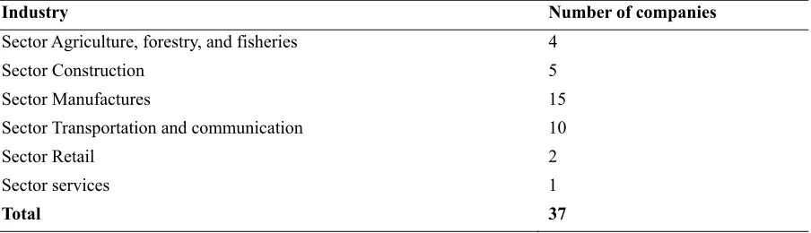
To our sample, three selection criteria were used: 1) the company must be listed on the Tunisian financial market, 2) the companies’ data must be observed on the longest possible period of study, 3) the company is not part of the financial sector given the peculiarities it represents in the field of regulation of financial reporting. The final sample thus constructed in this study is composed of 37 companies over the period 1998-2012.
The firms in our sample are part of six sectors: Sector Agriculture, forestry, and fisheries; Sector Construction; Sector Manufactures; Sector Transportation, communication; sector Retail; and Sector services.
Table 1. Distribution of firms by sector
Industry Number of companies
Sector Agriculture, forestry, and fisheries 4
Sector Construction 5
Sector Manufactures 15
Sector Transportation and communication 10
Sector Retail 2
Sector services 1
Total 37 3.2 Definition of variables
Accounting earnings and cash flows are collected directly from the financial statements composed of the balance sheet, state of result, state of cash flow and notes to the financial statements. The data were collected from the Financial Market Council Tunisia (FMC).
3.2.1 Operating Cash-flows (dependent variable)
For cash flows, it’s the cash flows from operating activities that are retained. Two methods were defined for the determination of operating cash-flow:
-The indirect method (as inspired by the SFAS n° 95 (1987)): According to this method, the operating cash-flow was generally approximated by the accounting earnings adjusted by the depreciation and provisions and the capacity of self-financing (variation in inventories; changes in operating receivables; Changes in operating liabilities).
-The direct method (as inspired by the SFAS n° 95 (1987)): Under this method, the Operating cash flow resulting from cash inflows and cash outflows from operating activities. Operating cash flow = cash inflow received from the customers – cash outflow liquidated to the suppliers – cash outflow of operating loads
3.2.2 Earnings
Variables in our study are as follows: NI: Net Income
OI: Operating Income CFO: Operating Cash Flow
All variables are divided by total assets. 3.3 Descriptive statistics
Table 2. Descriptive statistics of variables in the models (354 firms-years: 1998-2012)
Variables Mean SD Min Max
CFO 2.839472 19.43516 -37.65193 225.5934
NI 1.350238 11.20474 -44.36886 94.3214
OI 1.972882 14.68963 -38.53392 145.7202
CFO: Operating Cash Flow; NI : Net Income ; OI : Operating Income
The descriptive statistics presented above show that the average of operating cash-flows, net income and operating income are positive. These results are consistent with those already found in previous research (Sloan, 1996; and Barth et al. 2001). For the change in cash flows, it is the most important, these results are consistent with those Dechow (1994), Dechow, Kothari and Watts (1998) in the American context.
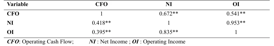
Table 3. The correlation matrix of Pearson (Spearman) above (below) the diagonal
Variable CFO NI OI
CFO 1 0.672** 0.541**
NI 0.418** 1 0.953**
OI 0.395** 0.835** 1
CFO: Operating Cash Flow; NI : Net Income ; OI : Operating Income ** Correlation is significant at the 1% level.
To measure the correlation between variables, we used the coefficient of Pearson and Spearman. Pearson correlations are used to signal that operating cash flows are positively and significantly correlated with net income (r = 0.672) and operating income (r = 0.541) at 1%. As regards the non-parametric correlations of Spearman, they can reveal a positive and significant correlation between cash flows, net income (r = 0.418) and the operating income (r = 0.395) at the 1%.
4. Models of research
According to Bowen, Burgstahler, and Daley (1986), there is no theory that allows specifying an appropriate form of a model for forecasting future cash flows. Lorek et al. (1993) suggest that the uni-varied model ARIMA which takes into account data quarterly cash flows provided more accurate forecasts for operating cash flows that cross-sectional multi-varied models used in previous studies (Wilson, 1986; Rayburn, 1986; Stober and Bernard, 1989). Lorek and Willinger (1996) showed that the pattern of multivariate time-series forecasting is the most efficient for the prediction of future cash flows.
In our study, models are built to the forecast horizon of one and two previous years. Thus, the dependent variable is represented by cash flows from operating activities to be provided by the independent variables of operating cash flow, net income and operating income. For the first level models, it is based on lagged values of one year. For the second level, it is late two previous years are retained. However, the third level model is based on multi-annual regressions, as developed previously by Greenberg, Ramesh and Johnson (1986), and Beth (1993). Forecasting models are as follows:
4.1 Forecast horizon of one year late
Model (1): , , ,
Model (2): , , ,
4.2 Prediction for the horizon two years late
Model (4): , , ,
Model (5): , , ,
Model (6): , , ,
4.3 Multi-annual forecast
Model (7): CFO, α α CFO, α CFO, ε,
Model (8): , , , ,
Model (9): , , , ,
5. The estimation techniques
In the case of panel data modeling, three techniques are used to estimate the coefficients namely the procedure Ordinary Least Squares (OLS), the fixed effect model and the random effects model.
For the first regression procedure, it is used for individual or temporal data. It can also be used for panel data, but it has the disadvantage of ignoring the double dimension. The second fixed-effects model, it is frequently used for panel data. It takes into account the heterogeneity of firms in the sample, and it assumes that the relationship between the dependent variable and the explanatory variables are the same for all individuals. The third random effects model is used for panel data. This model composed in error assumes that individual specificity is in a random form. The constant term specific to individual i is random. It consists of a fixed term and a random term specific to the individual to control individual heterogeneity.
By grouping the random terms of the model, we obtain a structure composed errors, ε i, t = μi + vit. Where μi denotes the random variable specific to the company, it takes into account the risk of the effect of heterogeneity, and it is invariant over time, while vit is the new error term.
It should be noted that for these two models (fixed effects / random effects), they take into account the heterogeneity between firms in the sample. However, it should be noted that before considering the heterogeneity, it is necessary to ensure the need to introduce this dimension in the estimate. For this purpose, a specification test individual effects is required. To choose the method most appropriate of panel data estimation, several tests must be performed. In first level, the specification test, thereafter the Hausman test.
5.1 The test of specification individual effects
The sample of this study is classified according the panel data, is characterized by the presentation of individual and temporal dimensions, (i) for companies and (t) for time. Thus, the first step of the estimate is to examine homogeneity or heterogeneity of the data generating process. In other words, is to examine whether the theoretical model is the same for all companies or whether there are specific effects of each company. This test is formulated as follows:
H0 : βi = β;
H
1 : βi ≠ β
The acceptance of H0 confirms the absence of a specific effect, and therefore, all firms are assumed to be homogeneous. As against, the acceptance of H1 provides evidence for the presence of heterogeneity across companies. This is the Fisher test that can verify or reject these hypotheses. With N the number of enterprises; T: the period of the study, and k the number of explanatory variables.
If the test is significant (p-value <5%), H0 is rejected, if not, H0 is accepted. If the null hypothesis is rejected (and therefore one must take into account the heterogeneity), one has to choose between the fixed effects model and random effects model.
5.2 The Hausman specification test
H0: E (ui | Xi) = 0 (estimators of model errors are effective).
H
1: E (ui | Xi) ≠ 0 (estimators of the model error component are biased). The Hausman test compares the variance-covariance of two estimators:
W must be positive, if not, we must invert the matrix, and begins with the random estimator. Under the null hypothesis of correct specification, this statistic is asymptotically distributed according to a chi-square with K degrees of freedom, the number of variable factors over time introduced in the model. If the test is significant (p-value <5%), it retains the estimators of the fixed effects model which are not biased. Otherwise, we use the error component model.
To evaluate the performance of prediction models, we first compare the adjusted R2. However, as stated by Watts and Leftwich (1977), a high adjusted R2 does not necessarily imply a higher predictive power. Therefore, in this study we consider the test of likelihood ratio. This test is a statistical test used to compare the robustness of two models among which the one is considered the null model, and the other the alternative model. This test is based on the ratio of likelihood which allows considering the performance of a model with regard to another one. Afterward, this ratio is used to calculate a p-value to decide whether to reject the null model in favor of the alternative model.
6. The empirical results
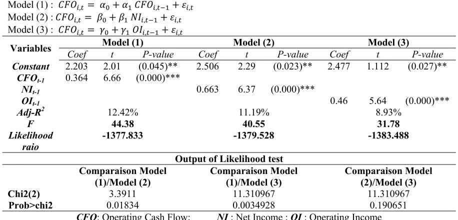
Panel A of Table 4 presents the estimation results of model (1), (2) and (3) related to the horizon of one year late. Estimates show that the coefficients of the three variables are positively significant for forecasting cash flows for the following year. R2 and the application of likelihood test ratio also prove the superiority of the model (1) with respect to model (2). Indeed, the statistical test is 3.3911 and the p-value associated with this test is low (below 10%). These results show that the cash-flows from operations are better than the net income to forecast future cash-flows. Similarly, comparing the model (1) with respect to model (3), the statistical test is 11.310967 and the p-value is 0, 0034. The test of likelihood shows that the cash-flows from operations are more relevant than the operating income for forecasting future cash-flows.
Therefore, according to these results, the cash flows from operating activities delayed by one year, which offers the most interesting predictions, which is contrary to the assertion of the FASB.
Table 4. The predictive power of net result, operating result with respect to cash flows to predict future cash flows: forecast horizon of one year late.
Panel A : Forecasting future cash flows with the late of one year delay cash flow from operations, net result and operating result
Model (1) : , , ,
Model (2) : , , ,
Model (3) : , , ,
Variables Coef t P-value Coef t P-value CoefModel (1) Model (2) Model (3) t P-value Constant 2.203 2.01 (0.045)** 2.506 2.29 (0.023)** 2.477 1.112 (0.027)**
CFOt-1 0.364 6.66 (0.000)*** NIt-1 0.663 6.37 (0.000)***
OIt-1 0.46 5.64 (0.000)***
Adj-R2 12.42% 11.19% 8.93%
F 44.38 40.55 31.78
Likelihood raio
-1377.833 -1379.528 -1383.488
Output of Likelihood test
Comparaison Model
(1)/Model (2) Comparaison Model (1)/Model (3) Comparaison Model (2)/Model (3)
Chi2(2) 3.3911 11.310967 11.310967
Prob>chi2 0.01834 0.0034928 0.190651
According to the panel B, the delay of two years indicates a predictive capability for the three variables of the study. This power is always positive for cash flows from operating, then it takes the negative sign for net income and operating income. For the model (4), we notice a loss of predictive performance relative to the model (1), contrariwise there was an improvement in accuracy between the model delay a single year and the two years.
Table 5. The predictive power of net result, operating result with respect to cash flows in predicting future cash flow: Forecast for the next two years of delay
Panel B: prediction of future cash flows with delay of two years of cash flow from operations, net result and operating result.
Modèle (4) : , , ,
Modèle (5) : , , ,
Modèle (6) : , , ,
Variables Model (4) Model (5) Model (6)
Coef t P-value Coef t P-value Coef t P-value Constant 1.704 1.77 (0.078)* 2.647 2.65 (0.008) 2.764 2.78 (0.006)***
CFOt-2 0.324 5.50 (0.000)*** NIt-2 -0.236 -2.08 (0.039)**
OIt-2 -0.292 -2.86 (0.005)***
Adj-R2 9.59% 11.9% 2.54%
F 30.27 4.32 8.19
Likelihood raio
-1157.517791 -1169.818884 -1167.915602
CFO: Operating Cash Flow; NI : Net Income ; OI : Operating Income
****: Significant at the 1% level, ** significant at the 5% level, significant at the 10% level.
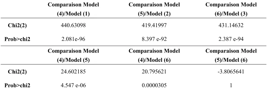
To delay two years of net result, estimates show an improvement in the performance of the model. The R2 passes of 11.19% for the model (2) to 11.9% for the model (4) and the likelihood ratio test indicates that the models which the explanatory variables delayed for two years are more efficient than models which explanatory variables lagged of one delay. Also, such test confirms the superiority of the delay of two years of the operating cash flows with regard of the two other variables. Indeed, the test statistic is 24.602185, and the associated p-value is 4.547 e-06 when we compare the model (4) with regard to the model (5) and it is 20.795621 and the associated p-value is 0.0000305 when we compare the model (4) with regard to the model ( 6 ). Also, this test is used to demonstrate that the model (6) is better than model (5).
Table 6. Output of Likelihood test
Comparaison Model (4)/Model (1)
Comparaison Model (5)/Model (2)
Comparaison Model (6)/Model (3)
Chi2(2) 440.63098 419.41997 431.14632
Prob>chi2 2.081e-96 8.397 e-92 2.387 e-94
Comparaison Model (4)/Model (5)
Comparaison Model (4)/Model (6)
Comparaison Model (5)/Model (6)
Chi2(2) 24.602185 20.795621 -3.8065641
Prob>chi2 4.547 e-06 0.0000305 1
According to the panel C, the addition of a further delay in the prediction models improves the predictive ability of the models compared to those associated with a horizon of one year. Indeed, for the three predictors we notice a marked improvement in the predictive ability of the models at the level of accuracy of their forecasts. For cash flow from operations, estimates of model (7) show that this dimension is positively significant for the prediction of future cash flows for the two years late. For the other two variables, the outputs show that the predictive ability is significant and positive for only one year behind, while she takes the negative sign for the second year. According to the adjusted R2 the model (8) based on delays of one and two years of net income offers the greatest performance. Table 7. The predictive power of net result, operating result with respect to cash flows to predict future cash flows: multi-annual models
Panel C: Forecasting future cash flows with delay of two years of the cash flow from operations, net result and operating result
Model(7): , , , ,
Modèle (8) : , , , ,
Modèle (9) : , , , ,
Variabls Coef Model (7) t P-value Coef Model (8) t P-value Coef Model (9) t P-value
Constant 0.964 1.09 0.277 1.9 2.19 (0.030) 2.042 2.33 (0.021)** CFOt-1 0,328 7,66 (0.000)***
CFOt-2 0.202 3.62 (0.000)***
NIt-2 0.7807 9.72 (0.000)*** NIt-1 -0.5106 -5.00 (0.000)***
OIt-1 0.582 9.15 (0.000)***
OIt-2 -0.549 -5.85 (0.000)***
Adj-R2 25.85% 26.33% 25.15%
F 47.6 50.15 47.20
Likeliho
od ratio -1126.956737 -1124.520307 -1127.258384 CFO: Operating Cash Flow; NI : Net Income ; OI : Operating Income
****: Significant at the 1% level, ** significant at the 5% level, significant at the 10% level.
These results confirm the assertion of the FASB and the interpretations provided by the accounting literature that certain components of earnings are related to strategies whose effects on the future cash flows that will be felt over a period exceeding one year later (Beth, 1993; Finger, 1994; and Barth et al., 2001).
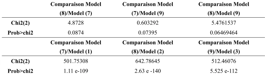
The likelihood test ratio reinforces also these interpretations. According to this test, it is the delayed of two years of net income that represent the most important predictor of future operating cash-flows. The superiority of the multi-variate models has been also proved by this test. Indeed, Looking below we see that the test statistic is 501.75308, and that the associated p-value is very low (1.11 e-109). The same interpretations have been deducted when we compare the model (2) to (8), and the model (3) to (9).
Table 8. Output of Likelihood test
Comparaison Model (8)/Model (7)
Comparaison Model (7)/Model (9)
Comparaison Model (8)/Model (9)
Chi2(2) 4.8728 0.603292 5.4761537
Prob>chi2 0.0874 0.07395 0.06469464
Comparaison Model
(7)/Model (1)
Comparaison Model (8)/Model (2)
Comparaison Model (9)/Model (3)
Chi2(2) 501.75308 642.78645 512.46076
Prob>chi2 1.11 e-109 2.63 e -140 5.525 e-112
7. Additional Analysis: The sensitivity of the results the sector of activity
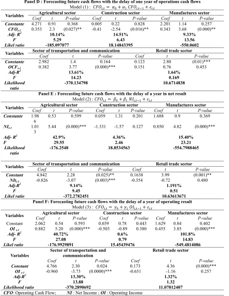
To test the susceptibility of estimates to the industrial sector, we re-estimate the models (1), (2) and (3) after corporate consolidation by industry. Our sample is the same by sector of activity, with the exception of the services sector has been excluded from our analysis because it includes a single company. The estimation results are summarized in Table 7. At the level of Panel D, the coefficient of cash flows operating in a previous year is significant for all sectors except retail sector. This coefficient is negative for the construction sector, while it is positive for other sectors. In Panel E, the result has a significant positive power for agriculture, and manufacturing. This variable shows no predictive ability for the building sector and the retail trade. In the model (3), which the estimates are summarized in panel F, all sectors illustrate a significant predictive capability except the building sector. This ability is positive for agriculture and manufacturing, and negative for the communication sector, electricity and gas.
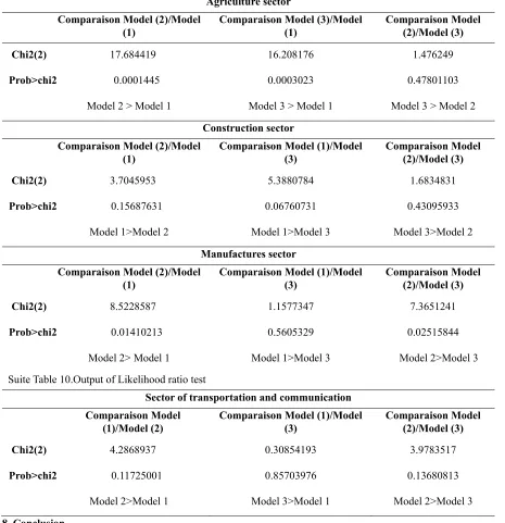
At the end to verify the performance of forecasting models, the application of the likelihood ratio test proves that for the agricultural sector, the model (3) is the most efficient one. Indeed, comparing the model (3) to the model (1), the value of the test is 16.201 and the associated p-value is 0.0003. The same interpretation is also deducted when comparing the model (2) with the model (3). In this case, the estimations indicate that the value of the test is 1.476 and the p-value is 0.478. Also, the likelihood ratio test allows to prove the superiority of the model (2) with regard to the model (1).
For the construction sector, it is the model (1) which demonstrates the most interesting performance according to the likelihood ratio test. In the same way, this last test justified the superiority of the model (3) with regard to the model (2). This test takes the value of 1.683 and a p-value of 0.4309. For the manufacturing sector, it is the model based on the net income which shows the most performance. Certainly, by comparing the model (2) with regard to the model (1), the test takes the value of 8.522 and the corresponding p-value is 0.0141. Similarly, by comparing the model (2) with the model (3) the test is 7.365 and the p-value is 0.0251. However, by comparing the model (1) and the model (3), it is the first one that demonstrates the most efficiency.
Table 9. The predictive power of net result, operating result relative to cash flows in predicts future cash flows: Analysis by sector of activity.
Panel D : Forecasting future cash flows with the delay of one year of operations cash flows
Model (1) : , , ,
Variables Agricultural sector Construction sector Manufactures sector
Coef t P-value Coef t P-value Coef t P-value
Constante 4.271 0.91 0.368 0.005 0.22 0.828 2.201 1.14 0.257
CFOt-1 0.353 2.3 (0.027)** -0.41 -2.54 (0.016)** 0.343 3.68 (0.000)**
Adj- R2 10.14% 14.51% 9.33%
F 5.29 6.43 13.56
Likel ratio -185.097077 18.14843395 -550.0602
Variables Sector of transportation and communication Retail trade sector
Coef t P-value Coef t P-value
Constante 2.982 1.4 0.164 0.123 2.80 (0.01)***
OCFt-1 0.382 3.77 (0.000)*** 0.151 0.76 0.453
Adj-R2 13.61% 1.64%
F 14.23 0.169
Likelihood ratio
-370.134798 10.6714838
Panel E : Forecasting future cash flows with the delay of a year in net result
Model (2) : , , ,
Variables Agricultural sector Construction sector Manufactures sector
Coef t P-value Coef t P-value Coef t P-value
Constante 1.98
6 0.53 0.599 0.059 1.31 0.201 1.688 0.9 0.369
NIt-1 1.01
3 5.44 (0.000)*** -1.331 -1.57 0.127 0.850 4.82 (0.000)***
Adj- R2 42.9% 4.36% 15.40%
F 29.55 2.46 23.21
Likelihood ratio
-176.2548 18.8534563 -554.7988465
Variables Sector of transportation and communication Coef t P-value Coef t Retail trade sector P-value
Constant 4.842 2.28 (0.025)** 0.1638 3.99 (0.001)**
NItt-1 -0.826 -3.07 (0.003)*** -0.354 -0.72 0.480
Adj-R2 9.14% 1.191%
F 9.45 0.51
Likel ratio -372.2782451 10.63613671
Panel F: Forecasting future cash flows with the delay of a year of operating result
Model (3) : , , ,
Variables Coef t P-value Coef t Agricultural sector Construction sector P-value Coef Manufactures sector t P-value
Constant 2.062 0.54 0.593 0.039 0.78 0.443 1.629 0.84 0.402
OI t-1 0.882 5.20 (0.000)*** -0.503 -0.89 0.380 0.455 3.85 (0.000)***
Adj- R2 40.72% 0.6% 101.8%
F 27.08 0.79 14.83
Likel ratio -176.9929891 15.45439476 -549.4814086
Variables Sector of transportation and communication Retail trade sector
Coef t P-value Coef t P-value
Constant 4.766 2.30 0.024 0.173 4.36 (0.000)***
OI t-1 -0.960 -3.73 (0.0000)*** -0.651 -1.16 0.257
Adj-R2 13.30% 1.32%
F 13.88 1.32
Likelihood ratio -370.2890692 11.07012407
CFO: Operating Cash Flow; NI : Net Income ; OI : Operating Income
Table 10. Output of Likelihood ratio test
Agriculture sector Comparaison Model (2)/Model
(1)
Comparaison Model (3)/Model (1)
Comparaison Model (2)/Model (3)
Chi2(2) 17.684419 16.208176 1.476249
Prob>chi2 0.0001445 0.0003023 0.47801103
Model 2 > Model 1 Model 3 > Model 1 Model 3 > Model 2
Construction sector Comparaison Model (2)/Model
(1)
Comparaison Model (1)/Model (3)
Comparaison Model (2)/Model (3)
Chi2(2) 3.7045953 5.3880784 1.6834831
Prob>chi2 0.15687631 0.06760731 0.43095933
Model 1>Model 2 Model 1>Model 3 Model 3>Model 2
Manufactures sector Comparaison Model (2)/Model
(1) Comparaison Model (1)/Model (3) Comparaison Model (2)/Model (3)
Chi2(2) 8.5228587 1.1577347 7.3651241
Prob>chi2 0.01410213 0.5605329 0.02515844
Model 2> Model 1 Model 1>Model 3 Model 2>Model 3
Suite Table 10.Output of Likelihood ratio test
Sector of transportation and communication Comparaison Model
(1)/Model (2)
Comparaison Model (1)/Model (3)
Comparaison Model (2)/Model (3)
Chi2(2) 4.2868937 0.30854193 3.9783517
Prob>chi2 0.11725001 0.85703976 0.13680813
Model 2>Model 1 Model 3>Model 1 Model 2>Model 3
8. Conclusion
This study's main objective is to verify the FASB assertion that information about earnings is generally more predictive of future cash flows than current cash flows. We rely on annual and multi-annual models, we offer in this study clarification on the role of earnings relative to cash flows past to forecasting future cash flows operating in the Tunisian context. In this study, we analyze a sample of 37 companies listed on the Tunisian financial market for the period 1998-2012.
Our analysis was later extended by studying the sensitivity of estimates to sector of activity. With the results of this review, we demonstrate that the predictive ability of accounting information vary across industrial membership. Indeed, estimates showed that operating cash flows that have the most significant predictive power for future cash flows in the transport sector, communication, electricity and gas. By contrast, it’s the earnings that is superior to the agricultural and manufacturing sectors. These findings confirm interpretations of Farshadfar and Monem (2013), Barth, Beaver and Landsman (2005), Barth et al. (2001), Dechow (1994).
The results of this study are interesting for users of financial statements (investors, financial analysts…), accountants’ professionals and all interested parties in accounting information and its relationship to future cash flows. For the users of financial statements, it provides them a clarification about the relevance of indicators for estimating the future corporate profitability, and therefore, it provides a proposal to improve the evaluation process and correct the forecast errors. For the standards, it illuminates them on the relevance of the information provided in financial statements and the transparency of the accounting disclosure systems.
Despite these contributions, this study is not without limits. Indeed, the sample is considered to be relatively restricted to generalize the findings. Similarly, studies of predictive capacity of accounting information on a sample of heterogeneous firms could be a source of bias in the results found, the fact that the predictive ability of information elements disclosed may depend on the economic circumstances and characteristics of companies.
References
Ali, A. (1994). The incremental information content of earnings, working capital from operations, and cash-flows. Journal of Accounting Research, Vol.32, pp.61-74. http://dx.doi.org/10.2307/2491387
Atwood, T.J., Drake, M.S., Myers, J.N., Myers, L.A. (2011). Do Earnings Reported Under IFRS Tell Us More About Future Earnings and Cash Flows? Journal of Accounting and Public Policy, Vol.30, pp.103-121. http://dx.doi.org/10.1016/j.jaccpubpol.2010.10.001
Barth, M.E., Cram, D.P., & Nelson, K.K., (2001). Accruals and the Prediction of Future Cash- Flows. The Accounting Review, Vol.76, Issue.1 pp.27-58. http://dx.doi.org/10.2308/accr.2001.76.1.27
Barth,M.E., Beaver, W.h., Hand, J.R.M., & Landsman, W.R. (2005). Accruals, accounting based valuation models, and the prediction of equity values. Contemporary Accounting Research, Vol.27, Issue.2, pp413-460.
Beaver, W.H. (1989). Financial Accounting: A Accounting Revolution. Englewood. Cliffs, NJ: Prentice-Hall. Belkaoui, A.R. (1984). Théorie comptable. Presses de l’Université du Québec. 2ème Edition 1984. pp.416.
Bowen, .R.D., Burgstahler., & Daley, L. (1987). The incremental information content of accruals versus cash-flows. The Accounting Review, Vol.62, Issue.4, pp.723-747.
Brown, L.D., & Pinello, A. (2007). To what extent does the financial reporting process curb earnings surprise games?
Journal of Accounting Research, Vol.45, Issue.5, pp.947–981. http://dx.doi.org/10.1111/j.1475-679X.2007.00256.x
Call, A., (2008). Analysts’ Cash Flow Forecasts and the Predictive Ability and Pricing of Operating Cash Flows. Working paper, University of Georgia.
Call, A.C., Chen.S., & Tong.Y.H. (2009). Are analysts’ earnings forecasts more accurate when accompanied by cash-flow forecasts. Review of Accounting Studies, Vol.14, Issue 2/3, pp.358-391. http://dx.doi.org/10.1007/s11142-009-9086-7
Cheng, C.S., Agnes, Liu, & Chao-Shin. (1997). The Value-Relevance of SFAS N°95: Cash-Flows From operations as Assessed By Security Market Effects. Accounting Horizons, Vol.11, pp.15-18.
Dechow, P.M, & Dichev, I.D. (2001). The quality of accruals and earnings: The role of accruals estimation errors. The Accounting Review, Vol.77, pp.35-59. http://dx.doi.org/10.2308/accr.2002.77.s-1.35
Dechow, P.M. (1994). Accounting earnings and cash-flows as measures of firm performance: The role of accounting accrual. Journal of Accounting and Economics, Vol.18, pp.3-42. http://dx.doi.org/10.1016/0165-4101(94)90016-7
DeFond, M.L. & Hung, M. (2003). An empirical analysis of analysts’ cash-flow forecasts. Journal of Accounting and Economics, Vol.35, pp.73-100. http://dx.doi.org/10.1016/S0165-4101(02)00098-8
Demski, J. S., & Sappington, D. E.M. (1990). Fully revealing income measurement. The Accounting Review, Vol.65, pp.363-383.
Farshadfar, S., & Monem, R., (2013). Further evidence on the usefulness of direct method cash-flow components for forecasting future cash-flows. The International Journal of Accounting, Vol.48, pp.111-133. http://dx.doi.org/10.1016/j.intacc.2012.12.001
Greenberg, R.R., G.L. Johnson & K. Ramesh (1986). Earnings versus cash-flow as a predictor of future cash- flow measures. Journal of Accounting, Auditing, and Finance, pp. 266-277.
Hammami, H., (2012). The use of reported cash-flows versus earnings to predict cash-flows: Preliminary evidence from Quatar. The Busines Sytems Review, Vol.1, pp.103-121.
Healy, P., & Palepu, K., (1993). The effect of firm’s financial disclosure strategies on stock prices. Accounting Horizons, Vol.7, pp.1-11.
Holthausen, R., & Leftwich, R. (1983). The economic consequences of accounting choice: Implications of costly contracting and monitoring. Journal of Accounting and Economics, Vol.5, pp.77-117. http://dx.doi.org/10.1016/0165-4101(83)90007-1
Krishnan, V.G., & Largay, J.A. (2000). The Predictive Ability of Direct Method Cash-Flow Information. Journal of Business Finance and Accounting, Vol.27,pp215-245. http://dx.doi.org/10.1111/1468-5957.00311
Mcinnis, J., & Collins, D. (2011). The effect of cash-flow forecasts on accrual quality and benchmark beating . Journal of Accounting and Economics, Vol.5, Issue 3, pp219-239. http://dx.doi.org/10.1016/j.jacceco.2010.10.005
Murdock, B., & Krause, P. (1989). An empirical investigation of the predictive power of accrual and cash-flow data in forecasting operating cash flow. Akron Business and Economic Review, Vol.20, pp.100-113.
Murdock, B., & Krause, P. (1990). Further evidence on the comparative ability of accounting data to predict operating cash flows. The Mid-Atlantic Journal of Business, Vol.26, pp.1-14.
Penman, S., (2001). Financial statement analysis & security valuation. McGraw-Hill Irwin, New York, NY.
Philipich, K., Costigan, M., et Lovata, L. (1994). The corroborative relation between earnings and cash-flow information. Advances in Accounting, pp.112-133.
Quirin, J., O’Bryan, D., & Wilcox, W. (1999). The corroborative relation between earnings and cash-flows. Quarterly Journal of Business and Economics, Vol. 38, pp.3-16.
Rayburn, J., (1986). The association of operating cash Flow and accruals with security returns. , Journal of Accounting Research, Vol.24, pp.112-133. http://dx.doi.org/10.2307/2490732
Schilit, H., (1993). How to detect accounting gimmicks and fraud in financial reports. New York; NY; MC Graw-Hill.
Vickrey, D. (1996). Additional thoughts on conditions for fully revealing disclosure. Journal of Business Finance and Accounting, Vol.23, pp.481-490. http://dx.doi.org/10.1111/j.1468-5957.1996.tb01135.x
Wasley, C., & Wu, J. (2006), Why do managers voluntarily issue cash flow forecasts? Journal of Accounting Research, Vol. 44, pp.389-429. http://dx.doi.org/10.1111/j.1475-679X.2006.00206.x
Watts, R.L, & Zimmerman, J.L. (1986). Positive Accounting theory. Prentice-Hall, (1986), 388 pages.