A Localization Algorithm of Wireless Sensor Network Based on Statistical Uncorrelated Vector

(1)

A Localization Algorithm of Wireless Sensor Network

Based on Statistical Uncorrelated Vector

https://doi.org/10.3991/ijoe.v13i07.7283

Min Wang

Hunan Mechanical & Electrical Polytechnic, Hunan, China

[email protected]

Abstract—For exploring wireless sensor network _{a self-organized}

net-work _{a new node location algorithm based on statistical uncorrelated vector}

(SUV) model, namely SUV location algorithm, is proposed. The algorithm, by translating the node coordinate, simplifies the solution to double center coordi-nate matrix, and gets the coordicoordi-nate inner product matrix; then it uses statistical uncorrelated vectors to reconstruct the coordinates of the inner product matrix and remove the correlation of inner matrix of coordinates caused by the ranging error, so as to reduce the impact of ranging error on subsequent positioning ac-curacy. The experimental results show that the proposed algorithm does not consider the network traffic, bust still has good performance in localization. At last, it is concluded that reducing the amount of communication of sensor nodes is beneficial to prolong the service life of the sensor nodes, thus increasing the lifetime of the whole network.

Keywords—wireless sensor, SUV, inner product matrix

1

Introduction

(2)

the signal intensity attenuation into the signal propagation distance. Since that the wireless signal, with the increase of transmission distance, the signal intensity will be reduced by a certain law. However, the propagation characteristics of signals are re-lated to environmental parameters, and the signal attenuation rule is affected by the temperature, humidity, obstacles, communication mode, multipath effect and other factors [2-3], so it is difficult to establish a unified signal transmission attenuation model. In addition, the RF antenna height is also an important factor affecting the signal transmission attenuation model. The accuracy of the localization algorithm based on RSSI is not only related to the ranging accuracy based on the signal intensi-ty, but also related to the characteristics of the localization algorithm. Many scholars have put forward a lot of RSSI positioning algorithms. For example, the famous RA-DAR positioning system, multi-point positioning method [4], the maximum a posteri-ori probability location algposteri-orithm based on the model and the map [5].

This paper is devoted to the study of location problem based on RSSI ranging. In order to reduce the influence of ranging errors on the positioning accuracy, a location algorithm based on statistical uncorrelated vector set (SUV) is proposed. The algo-rithm, by coordinate transformation, simplifies the solution equation of the center coordinate matrix, uses statistical uncorrelated vectors to reconstruct the coordinates of the inner product matrix and reduce the ranging noise interference, and directly uses the inner product matrix to calculate the coordinates of the nodes. The experi-mental results showed that the SUV location algorithm can effectively improve the positioning accuracy in the case of large ranging error, especially suitable for wireless sensor network node localization based on low cost hardware.

2

SUV location algorithm

2.1 Centralized SUV localization algorithm

A centralized location algorithm is an algorithm for focusing the desired infor-mation to a central node or a computer, and locating a single or all of the nodes. Sup-pose the original coordinate of N nodes X1X2…XNis

X

'_i

(

X

'_i

!

R

d

)

, and

the set N={1,2},... N} represents a collection of sensor nodes. All nodes are transi-tional, so

X

'₁ is at the origin of coordinate, the translation of

a

=

(

a

₁

,

a

₂

,...,

a

_d

)

, then the new coordinate is

X

_i

(

X

_i

!

R

d

)

, in which

X

'₁is an arbitrary node in the reference nodes, and then the coordinate matrix of reference node after transition is

[

]

T

N 2 1

N

X

=

,

,...,

. The 2-2 distance between all nodes forms a measurement

matrix

N N ij N

d

D

!

"

#

$

%

&

'

=

~ , where the measurement distance between the nodes is:

(

)

(

"

)

!

=

,

~

j i ij

N

d

x

(3)

In (1),

(

)

!

(

)

= " " "

#

=

d 1 2 j i j

i

x

d

,

is the Euclidean distance between the

sen-sor node Xi and Xj. In order to get the inner product between the coordinates of the

nodes, introduce the coordinate inner product matrix

N N ij N

d

B

!

"

#

$

%

&

'

=

, and bij is:

2

d

b

~2

ij ~ 2 j 1 ~ 2 i 1

ij

!!

/

"

#

$$

%

&

'

+

=

(2)

Because of the error of the measurement value

d

~_ij, the correlation of the data that is only correlated in the d dimension is extended to the high dimension, and the ei-genvalue decomposition of BN is performed, and the number of eigenvalues greater

than 0 will be greater than d. If only the first d eigenvalues and their corresponding eigenvectors are chosen to form the relative coordinate, the error will be larger.

In wireless sensor networks, because the BN is usually singular, there is at least one

eigenvalue of 0 for the BN feature decomposition, which leads to the in-existence of

the inverse matrix of the eigenvalue matrix. In the following, the eigenvalue decom-position of BN can be expressed as:

(

)

!!

"

#

$$

%

&

!!

"

#

$$

%

&

=

_T 2 T 1 2 1 2 1 N

V

D

0

D

V

B

,

(3)

Define

B

'_N

=

V

₁

D

₁

V

₁T, where D1 is a diagonal matrix composed of r eigenvalue

greater than 0, V1 is the matrix composed of the eigenvectors corresponding to the r

eigenvalue greater than 0, D2 is the diagonal matrix constituted by the rest N+1-r

eigenvalues, and V2 is the matrix constituted by the eigenvectors corresponding to the

eigenvalues of D2.

The coordinates of unknown nodes can be calculated by

X

_N

x

T_k

=

b

'_k:

(

)

' k T N 1 N T N T

k

X

b

x

!

=

₍₄₎

In (4),

!

"

#

$

%

&

=

' ' ' '

...

k m k 2 k 1 k

b

,

k

=

{

M

+

1

,

M

+

2

,...,

N

}

, then the absolute coordinate

(4)

a

x

'k

=

k

!

₍₅₎

2.2 Distributed SUV localization algorithm

The distributed localization algorithm only needs to communicate with the neigh-bor nodes during the positioning process and the location process is completed in the node. In the distributed SUV localization algorithm, only the coordinates of anchor nodes are used, and the distance information between unknown nodes and anchor nodes is specified, to make a distributed location of the specified unknown nodes.

It is assumed that in the wireless sensor, there are K anchor nodes {X1, X2,... Xk}, the original coordinate is

X

'_i

(

X

_i'

!

R

d

)

, and the set K={1,2,... K} represents a col-lection of K anchor nodes. Preform the coordinate translation of all anchor nodes, to make

X

'₁ located in the origin of coordinates, and the translation is a=(a1,a2,...,ad),

then re-set the new coordinate

X

_i

(

X

_i

!

R

d

)

, in which

X

'₁ is an arbitrary node of anchor node, and then the anchor node coordinate matrix after the translation is

[

]

T

K 2 1

X

=

,

,...,

. Because the anchor node coordinate information is known,

the distance between anchor nodes is determined. The 2-2 distance between the an-chor nodes forms a measurement matrix

D

_K

( )

d

_ij _K _K

!

=

, in which

(

)

!

=

"

" "

#

=

d

1

2 j i

ij

x

d

is the Euclidean distance between nodes,

i

,

j

!

K

.

Similarly, in order to get the product relationship between the node coordinates, in-troduce the coordinate inner product matrix of coordinates

( )

K K ij

K

b

B

=

_! , in which

bij is:

(

d

)

2

b

2

ij 2

j 1 2

i 1

ij

=

+

!

/

₍₆₎

In distributed location system, the unknown nodes, through two ways, get the pa-rameter a, DK and BK. One is to directly store the three parameter in the unknown

nodes, the other is through a wireless signal to seed to the unknown nodes. In wireless sensor networks, for arbitrary unknown node K+1, we can the measure distance

( ) ( ) ( )

~ , ~

, ~

,k 1

,

2 k 1

,...,

k k 1

1

d

+ + + between it and all the other anchor nodes by the ranging technology. We assume that the unknown nodes can communicate with all the anchor nodes.

Because

b

_ij

=

b

_ji, the coordinate inner product matrix BK+1 can be represented by

(5)

( ) ( ) ( ) ( ) ( ) ( )

!

"

#

$

%

&

=

+ + + + + + + 1 k 1 k 1 k k 1 k 1 1 k k k 1 k 1 1 k

b

B

b

B

, , , , ,

...

₍₇₎

Similar to the centralized SUV localization algorithm, BK+1 is usually singular, and

there is at least one eigenvalue of 0 when BK+1 is conducted with characteristics

de-composition, which will cause that the inverse matrix of eigenvalue matrix does not exist. In the following, the eigenvalue decomposition of Bn can be expressed as:

(

)

!!

"

#

$$

%

&

!!

"

#

$$

%

&

=

+ _T 2 T 1 2 1 2 1 1 k

V

D

0

D

V

B

,

(8) In (8), D1 is the diagonal matrix composed of r eigenvalues more than 0, V1 is the

matrix composed of the eigenvectors corresponding to r eigenvalues more than 0, D2

refers to the diagonal matrix composed of the rest of K+1-r eigenvalues, and V2 is the

matrix composed of the eigenvectors corresponding to the eigenvalues of D2.

Reconstruct the coordinate inner product matrix:

T 1 1 1 1

k

V

D

V

B

'+

=

(9)

Because

( )

_k T_k

k k ij

k

b

X

B

=

_!

=

, we can get:

( ) '(k 1)

T 1 k

k

x

b

X

₊

=

₊ ₍₁₀₎

Then the unknown node coordinate

x

₍T_k₊₁₎ can be calculated:

( )

(

)

Tk '(k 1)

1 k T k T 1

k

X

b

x

+

!

+

=

₍₁₁₎

In (11),

b

'_k₊₁

=

(

b

₁'_,₍_k₊₁₎

,

b

'₂_,₍_k₊₁₎

,...,

b

'₍_k₊₁_{) (}_,_k₊₁₎

)

T.

At last, through the coordinate transition, we can get the absolute coordinate of the unknown nodes is:

( )

x

( )

a

x

k+1

=

k+1

!

'

(6)

3

Experimental simulation

The distance measurement technology based on RSSI, by the strength of the RSSI signal received, makes use of signal propagation attenuation model to obtain the dis-tance between the signal point to the receiving point. Radio frequency signal is used in wireless sensor localization. Because the RSSI is easy to be affected by the envi-ronment and other factors, there is no fixed propagation error model. It is necessary to determine the model parameters according to the specific environment for on-site measurement.

Select the CC2430 chip as the main chip of the experimental node. CC2430 is the first 2.4 GHz RF system single chip in line with ZigBee technology [6], which adopts the CC2420 chip architecture, and integrates ZigBee RF front-end, memory and micro controller on a single chip. The current loss of the chip in working is 27mA, and the current loss is less than 27mA or 25mA in the receiving or transmitting mode. Hard-ware supports for CSMA/CA function, digital RSSI/LQI and powerful DMA func-tion. Each node can receive / transmit frequency signal; a node sends a signal, and the other node receives the signal sent and measures the RSSI. The parameters of the RSSI signal transmission error model are estimated in the lab.

3.1 RSSI signal transmission attenuation model [7].

Pij is defined as the signal strength (mW) of node j received by node i, and

assum-ing that Pij=Pji, Pij is a log normal random variable, and Pij(dBm)=10log10Pij obeys the

Gauss distribution:

(

)

(

)

2

)

dB ij

ij dBm ~NP dBm

P ,! ₍₁₃₎

(

)

0

(

)

p 10

(

ij 0

)

ij

dBm

P

dBm

10

n

d

P

=

!

log

/

₍₁₄₎

(

dBm

)

Pij refers to the energy average value (DB MW),

!

dBis the standard

devia-tion,

!

(

)

=

"

" "

#

=

d

1

2 j i

ij

x

d

is the Euclidean distance between the node i and the

node j, P0(dBm) indicates the energy received when the node has the distance of d0,

and np suggests the path loss coefficient related to environment.

Use CC2430 production nodes to receive and transmit RF signal, and measure the RSSI value to verify the above statistical model. To obtain the above model, three parameters must be determined: d0P0(dBm) and np. Usually, take d0=1 m, P0(dBm)

value is the RSSI value measured when the distance between the node Xi and the node

X2 is dij=1m. When d0 and P0(dBm) are determined, the node Xi and the node X2 are

placed in different positions, measuring the RSSI value for several times, substituting in (14) to calculate for several times, and the average value of np is obtained. So far,

(7)

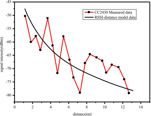
In Figure 1, the dot represents the average value of RSSI signal when sensor nodes are in different distance. In this experiment, 10 RSSI values are measured at each position, and then averaged. According to the measured value, we can get RSSI signal transmission attenuation model parameters: P0(dBm)!-45, np!3. Two parameters are

substituted in (14), we can get RSSI- distance data model as shown in the smooth curve in Figure 1.

0 2 4 6 8 10 12 14

-80 -75 -70 -65 -60 -55 -50 -45

signal

int

ens

ity(

dB

m

)

distance(m)

CC2430 Measured data RSSI-distance model data

Fig. 1. Relationship between RSSI signal intensity and distance

It is found that, for two fixed sensor nodes with a certain distance, not only RSSI will fluctuate, but the farther away from each other, the larger the fluctuation frequen-cy and amplitude. Figure 2 shows the distribution of the signal intensity with time when the transceiver is in the distance of 1, 2, and 3 meters, each position has a total of 105 sets of signals, and each signal is separated by 2s. We can see that the RSSI value fluctuates around the mean in a fixed position, and the greater the distance, the stronger the fluctuating. Figure 1 and Figure 2 show that the above model is in line with the actual situation.

3.2 Experimental results of SUV positioning based on RSSI

After the RSSI signal transmission attenuation model is obtained, the performance of the distributed SUV localization algorithm based on RSSI ranging is evaluated. Measurement environment is also selected in the laboratory. Eight reference nodes are placed around the laboratory of 10 x 10m2_{, and the equipment and furniture are}

(8)

Fig. 2. RSSI signal intensity fluctuations with time of two nodes at the distance of 1, 2, 3 me-ters

4

Results and Discussion

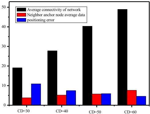
Figure 3 shows the relationship between CD and the average connectivity of the network, the average number of neighbor anchor nodes, and the positioning error. With the increase of 10m of CD, the average connectivity of the nodes in the network is increased by more than 10 nodes, and with the improvement of the network connec-tivity, the positioning error decreases.

0 10 20 30 40 50

CD=60 CD=50

CD=40 Average connectivity of network Neighbor anchor node average data positioning error

CD=30

(9)

In order to better evaluate the performance of the centralized SUV location algo-rithm, in the following, from the deployment number (NN) of sensor nodes, the rang-ing error between nodes ("), node communication distance (CD), we view the posi-tioning precision of the algorithm, as the standard for the evaluation of the posiposi-tioning performance of the algorithms proposed in this chapter. In the following three groups of experiments, the sensor nodes are randomly deployed in the area of 100 x 100m2_,

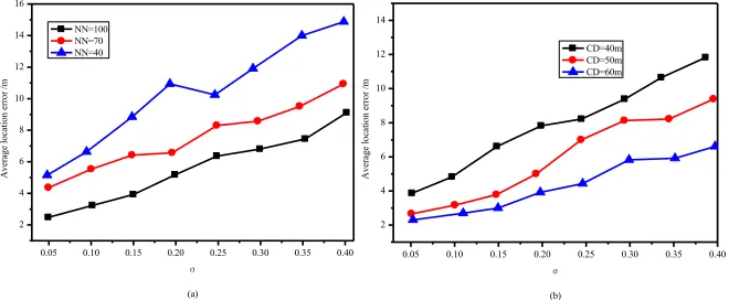
and we select any six of the nodes as the anchor node of the known coordinates. First of all, we evaluate the effect of NN on the performance of SUV localization algorithm. Figure 4 (a) is, in the case of range error "=0.1, to continue to add sensor nodes to the network, and get the positioning error graph of SUV algorithm. It can be seen that when the NN is more than 40, the positioning error of the three kinds of CD decreases; when the NN increases from 70 to 100, the three curves become more gentle. Taking CD=50 as an example, when NN=70, the average positioning error is 3.85M; when NN=100, the average positioning error is 3.23M, reduced by 0.62m.

Figure 4 (b) gives, when " changes, the relationship between average positioning error and NN. Similar to Figure 4 (a), the curve slope of NN between 30 to 40 is greater than the curve slope when NN is between 40 to 70, and the curve slope of NN between 40 to 70 is greater than the slope between 70 to 100. That is to say, when NN>70, under the same parameter conditions, the variation range of positioning error is no great, which provides a reference for the deployment of sensor networks. From Figure 4 (b), it can also be seen that, the influence of " on SUV positioning is rela-tively large (the spacing between the three curves is obvious). In the case of NN=80, the positioning error average values when " is 0.1, 0.2 and 0.3 were 3.26m, 6.11m, and 8.52m, respectively, and the positioning accuracy decreased significantly.

30 40 50 60 70 80 90 100 4

6 8 10 12 14 16 18

A

verage

locat

ion err

or

/m

Mumber of the sensor nodes (a)

CD=40m CD=50m CD=60m

30 40 50 60 70 80 90 100 4

6 8 10 12 14 16 18

A

verage

locat

ion err

or

/m

Mumber of the sensor nodes (b)

=0.1

=0.2

=0.3

Fig. 4. (a) the influence of the number of sensor nodes (b)the impact of sensor nodes on the positioning error under different ranging distance

(10)

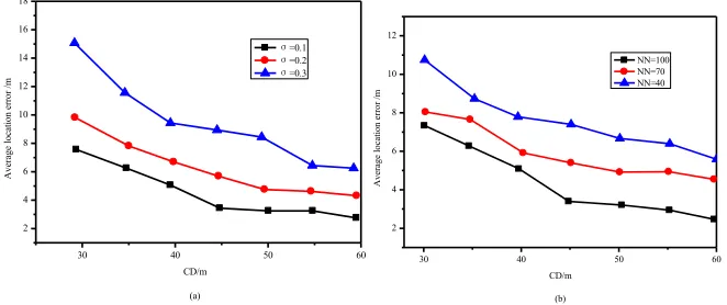
100 or 70, the change amplitude of the curve is slower than when NN is 40; in the three cases, when " increased from 5% to 40%, the positioning error was increased by 7.50 m, 6.63 m, and 10.92 m; it also verified the relationship between the number of node and the positioning error in the last group experiment. Then, set the NN=100 in the region, and in the case of CD of 40 m, 50 m, and 60 m, calculate the positioning error by changing ", and the results are shown in Figure 5 (b). It can be seen that the positioning error increases with the increase of "; when " increased from 0.05 to 0.40, the positioning error in three kinds of CD were increased by 8.10 m, 7.50 m, 5.03 m, respectively.

0.05 0.10 0.15 0.20 0.25 0.30 0.35 0.40 2

4 6 8 10 12 14 16

A

ve

rag

e

loc

at

ion

er

ror

/m

(a) NN=100

NN=70 NN=40

0.05 0.10 0.15 0.20 0.25 0.30 0.35 0.40 2

4 6 8 10 12 14

A

ve

rag

e

loc

at

ion

er

ror

/m

(b) CD=40m CD=50m CD=60m

Fig. 5. (a)the total number of different nodes (b) the influence of sensor node ranging error on positioning error under different node communication distance

(11)

30 40 50 60 2

4 6 8 10 12 14 16 18

A

ve

ra

ge

loc

at

ion e

rror

/m

CD/m (a)

=0.1

=0.2

=0.3

30 40 50 60

2 4 6 8 10 12

A

verage

locat

ion err

or

/m

CD/m (b)

NN=100 NN=70 NN=40

Fig. 6. (a) different ranging errors (b)the influence of the communication distance of the sensor nodes on the positioning error under different total number of nodes

5

Conclusion

The algorithm greatly simplifies the solution of center coordinate matrix and gets the coordinate inner product matrix, and uses statistical uncorrelated vectors to recon-struct the coordinates inner product matrix and the correlation of the coordinate inner product matrix caused by removing the ranging error. After the appropriate transfor-mation, the SUV localization algorithm can realize the wireless sensor node central-ized localization and the distributed localization two kinds of plans. We use TI com-pany's CC2430 as the main chip, design and produce relevant wireless sensor nodes. Based on these hardware nodes, a lot of tests are carried out to analyze the influence of the RSSI signal transmission attenuation model and the actual environment on the RSSI signal. The proposed algorithm does not consider the network traffic. In the process of positioning, reducing the amount of communication of sensor nodes is beneficial to prolong the service life of the sensor nodes, thus increasing the lifetime of the whole network. Under the premise of ensuring the positioning accuracy, it is of great significance to reduce the network traffic positioning technology as much as possible.

6

References

[1]Andreyev, P., Grishko, A., & Yurkov, N. (2016). The temperature influence on the

propa-gation characteristics of the signals in the printed conductors. International Conference on Modern Problems of Radio Engineering. Telecommunications and Computer Science (pp.376-378).

[2]Da-li, Z., Jing, S., Hao, J., & Ying, Y. (2016). Pseudo Base Location for Mobile Terminal

with Abnormal Dynamic Access. International Journal of Future Generation

(12)

[3]Guo, H., Zhang, H. (2017). Development of double-pair double difference earthquake lo-cation algorithm for improving earthquake lolo-cations. Geophysical Journal International,

208(1): 333-348. https://doi.org/10.1093/gji/ggw397

[4]Hui, J., Yang, Y., Hui, Y., & Luo, L. (2016). Research on Identify Matching of Object and

Location Algorithm Based on Binocular Vision. Journal of Computational and Theoretical

Nanoscience, 13(3): 2006-2013. https://doi.org/10.1166/jctn.2016.5147

[5]Jia, K., Li, M., Bi, T., & Yang, Q. (2016). A voltage resonance-based single-ended online

fault location algorithm for DC distribution networks. Science China Technological

Sci-ences, 59(5): 721-729. https://doi.org/10.1007/s11431-016-6033-2

[6]Wang, H., Tong, L., Yu, L., & Ben, H. (2015). The research of facial features localization

based on posterior probability deformable model. IEEE International Conference on

Mechatronics and Automation (pp.2392-2396). IEEE. https://doi.org/10.1109/icma.2015.7

237861

[7]Xu, Q. (2014). Design and development of a compact flexure-based, precision positioning

system with centimeter range. IEEE Transactions on Industrial Electronics, 61(2):

893-903. https://doi.org/10.1109/TIE.2013.2257139

[8]Yang, B., Lei, Y., & Yan, B. (2016). Distributed multi-human location algorithm using

na-ive Bayes classifier for a binary pyroelectric infrared sensor tracking system. IEEE Sensors

Journal, 16(1): 216-223. https://doi.org/10.1109/JSEN.2015.2477540

[9]Zhang, S., Gao, H., & Song, Y. (2016). A New Fault-Location Algorithm for

Extra-High-Voltage Mixed Lines Based on Phase Characteristics of the Hyperbolic Tangent Function.

IEEE Transactions on Power Delivery, 31(3): 1203-1212. https://doi.org/10.1109/TPWRD

.2015.2461678

[10]Zhang, Y., Liang, J., & Wang, P. (2016, August). Mutual impedance parameter modeling

and accurate location algorithm of angled space crossed transmission lines. In Electricity Distribution (CICED), 2016 China International Conference on (pp. 1-6). IEEE. https://doi.org/10.1109/ciced.2016.7576202

7

Author

Min Wang is with Hunan Mechanical & Electrical Polytechnic, Hunan, China ([email protected]).