Cloud-based Geophysical Inversion Modeling Using GNU Octave and MatlabMPI on Amazon EC2

Cloud-based Geophysical Inversion Modeling Using

GNU Octave and MatlabMPI on Amazon EC2

https://doi.org/10.3991/ijoe.v13i09.7468

Jie Xiong

Yangtze University, Jingzhou, China; Mississippi State University, Starkville, MS, USA

Song Zhang

Mississippi State University, Starkville, MS, USA

Yuantao Chen!!_"

Changsha University of Science and Technology, Changsha, China

[email protected]

Abstract—Computer modeling and simulation can be very demanding in terms of computational resources. Cloud computing has opened up new avenues for the scientific researchers with limited resources to do complicated simula-tion. In order to investigate whether cloud computing is suitable for modeling and simulation, we first describe how to build a cloud-based modeling and sim-ulation platform using GNU Octave and MatlabMPI on the Amazon Elastic Compute Cloud (EC2). Then, we evaluation its performance taking the geo-physical inversion modeling as an example. The results show that the cloud-based modeling and simulation platform is suitable for basic modeling for free. It can provide much more higher performance with acceptable price. Further-more, we can cut down the cost by employing the Spot instance without losing the computation performance.

Keywords—Cloud-based modeling, Amazon Elastic Compute Cloud (EC2), Geophysical inversion modeling, GNU Octave, MatlabMPI

1

Introduction

and may expand or shrink based on demand [3]. Cloud computing has opened up new avenues for scientists with limited resources to do complicated simulation which hitherto required expensive and computationally-intensive resources [4].

The field of modeling and simulation tools is diverse and emergent. General-purpose tools (e.g. MATLAB [5] or Octave [6]) sit beside highly focused and do-main-specific applications [7]. MATLAB is a powerful general-purpose tool and widely employed to solve the scientific and engineering problems [8], including mod-eling and simulation [9-13]. However, using MATLAB on the cloud need MATLAB Distributed Computing Server license, which is very expensive, depending on the number of nodes used (See the white paper [14] for the detail of installation, configu-ration, and setting up clustered environments using licensed products from Math-Works on Amazon EC2).

GNU Octave is a high-level interactive language, primarily intended for numerical computations that is mostly compatible with MATLAB [6]. With Octave, which is developed under GNU license, the commercial license problems are solved. The MatlabMPI [15] is a set of MATLAB scripts that implement a subset of Message Passing Interface (MPI) and allow any MATLAB program, or Octave program (re-ported by [16]), to be run on a parallel computer .

Amazon EC2 could be used to build a virtual cluster, powerful enough for scien-tific computing, for free [17]. This paper is dedicated to study how to build a cloud-based modeling and simulation platform using GNU Octave and MatlabMPI on the Amazon EC2, and to validate its performance taking the geophysical inversion mod-eling as an example.

2

Building simulation platform on Amazon EC2

2.1 Building virtual cluster on Amazon EC2

Fig. 1. Architecture of the virtual cluster on Amazon EC2 (According to [17] ).

2.2 Deploying GNU Octave and MatlabMPI on the cloud (1) Start and launch a virtual cluster on Amazon EC2

$

starcluster start mycluster

$ starcluster sshmaster mycluster -u sgeadmin

(3) Install MatlabMPI

There are 3 steps to install MatMPI:

Step 1: Copy MatlabMPI into a location that is visible to all computers. Step 2: Add MatlabMPI/src directory to Octave path.

octave:1> addpath ~/MatlabMPI/src

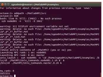
Step 3: Go to the ‘examples’ directory, and run a test program to validate the in-stallation.

octave:2> cd ~/MatlabMPI/examples

octave:3> eval (MPI_Run( ‘xbasic’, 2, machines );

MPI_Run has three arguments: the name of the MatlabMPI program ( without the “.m” suffix), the number of machines to run the program on and the “machines” ar-gument which contains a list of names of machines on which to run the program.

The “machines” argument can be of the following form: machines = {}; //Run on a local process.

machines = {‘machine1’, ‘machine2’}; //Run on multiprocessors. The result of running the ‘xbasic.m’ program is shown as following:

3

Cloud-based geophysical inversion modeling

3.1 General description

The magnetic method is one of the most popular geophysical techniques for the exploration of minerals, oil and gas resources [19]. Inversion is one of the important works of magnetic data quantitative interpretation. The magnetic inversion, same as the other geophysical inversions, is an ill-posed problem because the inversion result is non-uniqueness. The Tikhonov regularization is used to solve ill-posed geophysical inversion problem [20], which has two major issues must be studied: (1) How to choose the optimal regularization parameter; (2) How to find the global optimal solu-tion which independent on the initial guess.

J. Xiong and T. Zhang proposed a multiobjective optimization (MO) inversion al-gorithm deal with these two issues at the same time, but has the disadvantage of huge computational time [21]. We implement the MO inversion algorithm on the cloud-based modeling and simulation platform, described in chapter 2 in this paper, to over-come the problem of computational time mentioned above.

3.2 Problem formulation

Forward Modeling. We consider the 2D magnetic forward modeling. We divide the subspace into several regular arranged 2D prisms. The magnetic anomaly of a prism, which is shown in Fig. 3., is calculated as follows:

F=2kFe[sin(2I)sin!ln(r2r3/r4r1)+(cos2I!sin2! "sin2I)(#1" #2" #3+#4)] (1)

In the equation (1) where

F

is the magnetic anomaly,

F

_eis the Earth’s magnetic filed (EMF) intensity,

k

is the susceptibility contrast between the magnetic target and the host medium,

I

is the inclination of the EMF field,

!

is the strike angle of the prism relative to the magnetic north, and

r

_i

,

!

_iare distances and angles (see Fig. 3).

The magnetic anomaly vector is

F

=

(

F

₁

,

F

₂

,...,

F

_n

)

T, where

F

_i

(

i

=

1

,..,

n

)

is the magnetic anomaly on the

i

-th observation point on the surface. The model vector is

m

=

(

k

₁

,

k

₂

,...,

k

_m

)

T, where

k

_i

(

i

=

1

,...,

m

)

is the susceptibility of

i

-th prism. The magnetic anomaly vector

F

can be regarded as the model vector

k

multiplied by the kernel matrix

A

_(m!n). Equation (1) can be rewritten as

Am

F

=

(2)

3.2.2 Inversion Modeling

The goal of the inversion is to derive a model

m

that best fits the observed data. The objective function of the data misfit is [21]

min,

)

(

2

1

m

=

F

obs

"

Am

!

f

₍₃₎

Where

F

obsis the observed magnetic anomaly and

Am

is the theoretical predic-tion based on the model

m

.

The model constraint

f

₂

(

m

)

and regularization factor

!

are used to stabilize the inversion process and deal with non-uniqueness. The objective function of the regu-larization inversion is [20]

min

)

(

)

(

)

(

m

=

1

m

+

2

m

!

P

"

f

"

f

, (4)

where most common model constraint is minimum of norm of model vector:

2 2

(

m

)

=

m

f

₍₅₎

The regularization factor, which determines the relative weight of data misfit and model constraint, affects the inversion result extremely.

Because of the difficulty to choose the optimal regularization factor, J. Xiong and T. Zhang employ the MO inversion method to minimize the data fitness and model constraint simultaneously [21]. The MO objective function is

min

))

(

),

(

(

)

(

m

=

₁

m

₂

m

!

3.3 Modeling method

J. Xiong and T. Zhang employed a multiobjective particle swarm optimization inversion (MPSO-I) algorithm to solve the equation (6) successfully except the disadvantage of huge computational time [21].

In the MOPSO-I algorithm, the swarm consists of N particles. The particle’s position and speed are updated as follows:

k i k i k i k i k i k i k i k

i

c

r

c

r

v

m

m

m

LEADER

m

pbest

v

v

+

=

!

+

!

+

"

=

+ + 1 2 2 1 1

1

#

(

)

(

),

(7)

where

m

k_i

,

v

k_i

,

pbest

k_iis the position, speed, and personal best of the i-th par-ticle at the k iteration;

LEADER

is the global best of the swarm at the k itera-tion.

!

is the inertial weight;

r

₁

,

r

₂are random numbers between 0 and 1; and

2 1

,

c

c

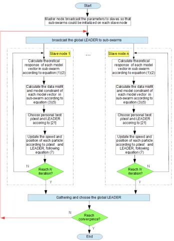
are factors.

Here, we propose a parallel MPSO-I algorithm and implement it on the cloud-based modeling and simulation platform using GNU Octave and MatlabMPI on the Amazon EC2, to overcome the computational time problem. The cloud-based geophysical inversion modeling algorithm is illustrated in Fig.4.

In the Fig.4, we can see that there are three main steps in the algorithm: (1) the master node broadcast the necessary parameters to slave nodes, including the sub-swarm size, local iteration number N, upper and lower boundary of susceptibility,

!

,

,

I

F

_e , so that each slave node could initial a swarm locally; (2) each sub-swarm iterated locally on slave node for N iterations; (3) master node gathering information and choose global LEADER.

4

Numerical Results

Table 1. Computation time and price of several typical instance types

Instance Type

Computation time (seconds) Price ($/hour) 1 node 2 nodes 4 nodes 8 nodes 16 nodes On-Demand _instance Spot in-_stance

PC 4381.1 -- -- -- -- -- --

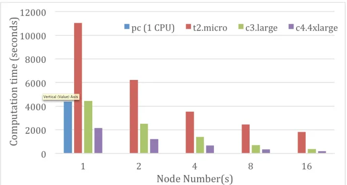
t2.micro 11045.3 6231.7 3541.1 2439.2 1821.9 free -- c3.large 4453.7 2498.0 1388.3 714.4 378.7 0.105 0.0156 c4.4xlarge 2142.8 1205.9 671.7 345.3 178.8 0.796 0.1887

The comparing of geophysical inversion modeling computation time between PC and different types of instance are illustrated in Fig.5.

From Table 1 and Fig. 5 we can see that: (1) Although t2.micro instance is less powerful than comparing PC, the cluster of t2.micro instances is more powerful than PC and it is free. (2) The one node c3.large instance cluster is as powerful as PC and c4.4xlarge instance is more powerful than PC. Furthermore, the cluster of c3.large instances and c4.4xlarge instances are much more powerful than PC; (3) The prices of c3 large and c4.4xlarge instance is 0.105 and 0.796 $/hour for On-Demand instance respectively, and 0.0156 and 0.1887 $/hour for Spot instance respectively, which are all affordable for scientific researchers.

To investigate the price issue in detail, we calculate the total prices for 100 times modeling on Amazon EC2 for different types of instance, and list the results in Table 2. The total prices vary from free to $63.26, according to instance types with different computation abilities and the size of cluster.

Table 2. Total prices for 100 times modeling on the Amazon EC2 for different types of in-stance

Instance Type Total Price ($)

1 node 2 nodes 4 nodes 8 nodes 16 nodes

t2.micro free free free free free

c3.large (On-demand) 12.99 14.57 16.20 16.67 17.67 c4.4xlarge (On-demand) 47.38 53.33 59.41 61.08 63.26

c3.large (SPOT) 1.93 2.16 2.41 2.48 2.63

c4.4xlarge (SPOT) 11.23 12.64 14.08 14.48 15.00

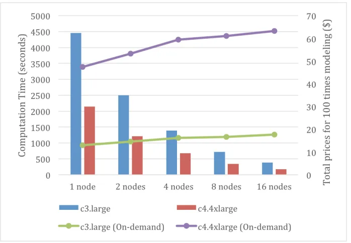
We put the computation time data in Table 1 and total price data in Table 2 togeth-er and plot the Fig.6 and Fig. 7, to show the relationship of them. From Fig. 6, we can see that, for the On-Demand instance(s), the computation time of geophysical inver-sion modeling on the cluster of c4.4xlarge instance(s) is about half of that of c3.large instance(s), however the total price of c4.4xlarge instance(s) is about 3 times of that of c3.large instance(s). This results indicate that if we do not care about the computa-tion time very much, the price of relative lower performance instance is more ac-ceptable.

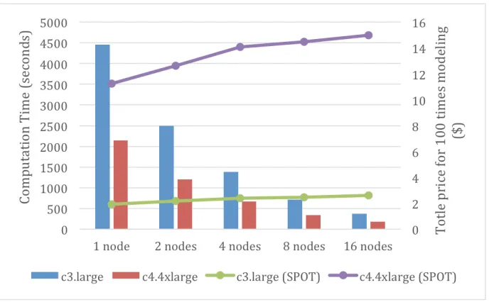
Fig. 7. Computation time and total prices for different types of Spot instances (100 times modeling) of cloud-based geophysical inversion modeling

The price of Spot instance is much more cheaper than that of On-Demand instance. From Fig. 7 we can see that, for the Spot instance(s), the computation time of geo-physical inversion modeling on the cluster of c4.4xlarge instance(s) is about half of that of c3.large instance(s), however the total price of c4.4xlarge instance(s) is about 4 times of that of c3.large instance(s). This results indicate that if we do not care about the computation time very much, the price of relative lower performance Spot in-stance is much more acceptable.

5

Conclusion

much more cheaper than On-Demand one(s). We could build a cloud-based modeling and simulation platform based on the Spot instance to do complicated modeling without spending too much money.

6

References

[1]X. Liu, Q. He, X., Qiu, et al., (2012). “Cloud-based computer simulation: Towards plant-ing existplant-ing simulation software into the cloud”, Simulation Modellplant-ing Practice and Theo-ry, Vol. 26, pp. 135-150. https://doi.org/10.1016/j.simpat.2012.05.001

[2]G. D’Angelo, M. Marzolla, (2014). “New Trends in parallel and distributed simulation: From many cores to Cloud Computing”, Simulation Modelling Practice and Theory, Vol. 49, pp. 320-335. https://doi.org/10.1016/j.simpat.2014.06.007

[3]F. Durao, J. F. S. Carvalho, A. Fonseka, et al., (2014). “A systematic review on cloud computing”, The Journal of Supercomputing, Vol. 68, No. 3, pp.1321-1346. https://doi.org/10.1007/s11227-014-1089-x

[4]S. Shekhar, H. Abdel-Aziz, M. Walker, et al., (2016). “A simulation as a service cloud middleware”, Annals of Telecommunications, Vol. 71, No. 3-4, pp. 93-108. https://doi.org/10.1007/s12243-015-0475-6

[5]The Mathworks (2017), “Matlab - The Language of Technical Computing”, http://www.mathworks.com/products/matlab, (Jul. 19, 2017, last accessed).

[6]https://www.gnu.org/software/octave, (Jul. 19, 2017, last accessed).

[7]S. Fortmann-Roe, (2014). “Insight Maker: A general-purpose tool for web-based modeling & simulation”, Simulation Modelling Practice and Theory, Vol. 47, pp. 28-45. https://doi.org/10.1016/j.simpat.2014.03.013

[8]T. Michalowsk, (2011). “Application of MATLAB in science and engineering”. Intech. https://www.intechopen.com/books/applications-of-matlab-in-science-and-engineering, https://doi.org/10.5772/1534 (Jul. 19, 2017, last accessed).

[9]A. Singh, R. Dehiya, P. K. Gupta, et al., (2017). “A Matlab based 3D modeling and inver-sion code for MT data”, Computer & Geosciences, Vol. 104, pp. 1-11. https://doi.org/10.1016/j.cageo.2017.03.019

[10]M. Dehghanimohammadabadi, T. K. Keyser, (2017). “Intelligent simulation: Integration of SIMIO and MATLAB to deploy decision support systems to simulation environment”, Simulation Modelling Practice and Theory, Vol. 71, pp. 45-60. https://doi.org/10.1016/j.simpat.2016.08.007

[11]Y. Liu, X. Zhou, Z. You, et al., (2017). “Discrete element modeling of realistic particle shapes in stone-based mixtures through MATLAB-based imaging process”, Construction and Building Materials, Vol. 143, pp. 169-178. https://doi.org/10.1016/j.conbuildmat.2017. 03.037

[12]Z. Abdin, C.J. Webb, E.M. Gray, (2016). “PEM fuel cell model and simulation in Matlab– Simulink based on physical parameters”, Energy, Vol. 116, Part 1, pp.1131-1141. https://doi.org/10.1016/j.energy.2016.10.033

[13]T. Wilberforce, Z. EI-Hassn, F.N. Khatib, et al., (2017), “Modelling and simulation of Pro-ton Exchange Membrane fuel cell with serpentine bipolar plate using MATLAB”, Interna-tional Journal of Hydrogen Energy, In press, Corrected proof, Available online Jun. 30, 2017.

[14]The Mathworks, (2017). Parallel Computing on the Cloud with MATLAB,

[15]http://www.ll.mit.edu/mission/cybersec/softwaretools/matlabmpi/matlabmpi.html , (Jul. 19, 2017, last accessed).

[16]X. Wu, (2013). “IAMCS Introduction to Parallel Programming with MPI + Matlab/Octave, IAMCS Tutorials”, http://faculty.cs.tamu.edu/wuxf/talks/IAMCS-ParallelProgramming-2013-3.pdf , (Jul. 19, 2017, last accessed).

[17]J. Xiong, S. Shi, S. Zhang, (2017). “Build and evaluate a free virtual cluster on Amazon Elastic Compute Cloud for scientific computing”, International Journal of Online Engi-neering, Vol. 13, No. 8, pp.121-132. https://doi.org/10.3991/ijoe.v13i08.7373

[18]http://star.mit.edu/cluster/, (Jul. 19, 2017, last accessed).

[19]M.N. Nabighian, V.J.S. Grauch, R.O. Hansen, et al., (2005). “The historical development of the magnetic method in exploration”, Geophysics, Vol.70, pp.33ND-61ND.

[20]M.S. Zhdanov, (2002), “Geophysical inversion theory and regularization problems”, Vol-ume 36 (Methods in Geochemistry and Geophysics), Elsevier, Science.

[21]J. Xiong , T. Zhang, (2015). “Multiobjective particle swarm inversion algorithm for two-dimensional magnetic data”, Applied Geophysics, Vol.12, No.2, pp.127-136. https://doi.org/10.1007/s11770-015-0486-0

7

Acknowledgments

This work is support by the National Science Foundation of China (No. 61273179, No. 61673006), and Science and Technology Research Project of Education Depart-ment of Hubei Province of China (No. D20131206, No. B2016034, No. 20141304).

8

Authors

Jie Xiong received his Ph.D. Degree in geophysics and Information Technology from China University of Geosciences in 2012. He was a visiting professor at De-partment of Computer Science and Engineering, Mississippi State University, USA during 2016. He currently is an associate professor at School of Electrical Infor-mation, Yangtze University, China. His research interests include cloud computing, scientific visualization, and applied geophysical inversion theory.

Song Zhang received his M.S and Ph.D Degree in Computer Science from Brown University in 2000, 2006, respectively. He has been an associate professor at Depart-ment of Computer Science and Engineering, Mississippi State University, USA. His research interests include scientific visualization, data analysis, medical imaging, and computer graphics.

Yuantao Chen (corresponding author) received his Ph.D. Degree in Control Sci-ence and Engineering from Nanjing University of SciSci-ence and Technology in 2014. He currently is an associate professor at School of Computer and Communication Engineering, Changsha University of Science and Technology, China. His research interests include image processing, big data, and pattern recognition.