An Algorithm of Mobile Robot Node Location Based on
Wireless Sensor Network
https://doi.org/10.3991/ijoe.v13i05.7044
Peng An
Ningbo University of Technology, Zhejiang, China [email protected]
Abstract—In the wireless sensor network, there is a consistent one-to-one match between the information collected by the node and the location of the node. Therefore, it attempts to determine the location of unknown nodes for wireless sensor networks. At present, there are many kinds of node localization methods. Because of the distance error, hardware level, application environ-ment and application costs and other factors, the positioning accuracy of vari-ous node positioning methods is not in complete accord. The objective function is established and algorithm simulation experiments are carried out to make a mobile ronot node localization. The experimnettal results showed that the pro-posed algorithm can achieve higher localization precision in fewer nodes. In addition, the localization algorithm was compared with the classical localization algorithm. In conclusion, it is verified that the localization algorithm proposed in this paper has higher localization accuracy than the traditional classical local-ization algorithm when the number of nodes is larger than a certain number.
Keywords—wireless sensor, mobile robot node location, algorithm optimiza-tion
1
Introduction
The general conditions of the mobile robot working environment is complex, and some areas are not even suitable for human to stay, so in order to ensure that the robot can successfully complete the task, the operator needs to control the real-time location of their work [1]. Therefore, the mobile robot needs to be tracked and positioned during operation. Wireless sensor networks have the function of mutual positioning between nodes, and mobile robots can only be tracked by the corresponding position-ing service, and then complete the task [3]. Therefore, it is very important in practice to apply the localization function of wireless sensor networks to the localization of mobile robots [6].
sen-sor nodes is the primary condition for the monitoring of the location information ser-vice [2]. The nodes are placed on the mobile robot, they constitute a mobile wireless sensor network nodes, so the localization problem of the mobile robot can be trans-formed into the problem of locating the nodes on the robot.
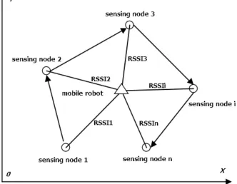
In the wireless sensor network, the general structure is shown in figure 1. On the one hand, the nodes participating in the work are limited in the energy supply due to the condition, and because of this reason, its function will be greatly reduced [4]. On the other hand, because of the low cost of node production, a large number of nodes have to be involved to complete the task. This poses a very high requirement for the localization technology and localization algorithm of unknown nodes. Therefore, it is necessary to develop a scientific and effective localization algorithm for mobile ro-bots based on the inherent characteristics of low energy consumption, low production cost, insufficient storage and communication capacity, and computational capability of the mobile robot [5].
Wireless AP Sink nodes
Energy supply module
Wireless communication module Sensor module
Management node
Processor module Global Internet
Fig. 1. The node structure and system structure of the sensor network
2
State of the art
In 1978, the US Defense Advanced Research and Planning Agency (DARPA) funded the Carnegie Mellon University's Distributed Sensor Network Working Group to study the technology of distributed wireless sensor networks. In 1990, DARPA launched a low-power Wireless Integrated Microsensors (LWIM) program, and de-signed CMOS integrated micro-system technology miniaturized low-power wireless sensor. Later, in 1993, it launched a wireless integrated network sensor (referred to as WINS) research program. The program mainly studies the microelectromechanical system sensor communication circuit, networking protocol and processing architec-ture. In 1998, under the support of DARPA and other institutions, the mainstream of the United States launched a smart dust program. The program enables highly inte-grated computing devices with sensing and communication. There is a cubic millime-ter size of the micro-sensor.
Compared with some developed countries, the research of wireless sensor net-works in China is relatively late, but the development is very rapid. The research on wireless sensor networks mainly focuses on miniaturization and intelligentization of sensor nodes, topology control, network protocols (including routing protocols and MAC protocols), node location and target tracking, data fusion, Qo S protection and reliability design, and network security and so on. Most of the domestic research still stays at the simulation level. Due to the fact that the actual environment is complex and uncertain, there is still a big gap from the practical application.
In summary, most of the above-mentioned positioning algorithms require expen-sive equipment to support the operation of the algorithm, and it is critical to the stabil-ity of the environment. Therefore, in this paper, we proposed a localization method for mobile robot nodes, and carried out the simulation experiment. In the simulation experiment, after selecting the objective function, the algorithm is optimized by the ranking method. The experimental results show that the proposed algorithm can achieve higher localization precision in fewer nodes. In this paper, the environmental parameters, namely the path loss factor k, are calculated, and the calculated value of k is simulated and analyzed by using the optimized localization algorithm. At last, this paper compared the localization algorithm with the classical localization algorithm.
3
Environmental parameters
In the calculation, we need to determine the two parameter values: environment pa-rameter k and node papa-rameter P + G, that is, the path attenuation factor, the transmis-sion power P of the node and the antenna reception gain G of the node (with respect to the node, the relative change is not large), but K changes with the change of the external environment, and has a great influence on the measurement results, so it needs to be calibrated in time.
In the case where the different receivers are away from the source distance d, the RSSI values are tested by the following equations:
!
"
!
#
$
%
+
=
&
+
&
+
=
&
+
=
)
(
)
(
)
log(
10
)
log(
10
44
.
32
)
(
)
/
log(
10
)
(
)
(
0 0 0 0d
PL
G
P
RSSI
f
k
d
k
d
PL
d
d
k
d
PL
d
PL
There are n measurement positions, d=d1, d2, ... , dn, respectively, the following equations can be obtained:
!
!
"
!
!
#
$
+
=
%
+
%
+
%
&
+
=
%
+
%
+
%
&
+
=
%
+
%
+
%
&
44
.
32
))
log(
10
)
log(
10
)
/
log(
10
(
44
.
32
))
log(
10
)
log(
10
)
/
log(
10
(
44
.
32
))
log(
10
)
log(
10
)
/
log(
10
(
0 0 2 0 0 2 1 0 0 1 nn
d
d
f
RSSI
d
k
!
RSSI
f
d
d
d
k
!
RSSI
f
d
d
d
k
!
!
Among them: ! ! ! ! ! ! " # $ $ $ $ $ $ % & ' ( ' ( ' ( ' ( ' ( ' ( ' ( ' ( ' ( = (f ) (d ) /d n (d (f) ) (d ) /d (d (f) ) (d ) /d (d A log 10 0 log 10 0 log 10 1 log 10 0 log 10 0 2 log 10 1 log 10 0 log 10 0 1 log 10 1 ! ! ! ! ! ! ! " # $ $ $ $ $ % & + + + = 44 . 32 44 . 32 44 . 32 2 1 RSSIn RSSI RSSI B !B
A
A
A
X
k
X
G
P
TT
!
!
!
=
=
+
=
"1)
(
]
,
[
$
#$
The value of the environmental parameter k is often estimated empirically. The ac-tual environment parameters and unknown nodes in the simulation process can be set manually. This section uses the following process for simulation:
Fig. 2. Parameter calibration schematic
In the Figure 2, we first select the environment parameter k in a real environment, and then set the unknown node location and combine the actual environment parame-ters with the above formula to generate a large number of beacon nodes' position and signal strength information. By using the generated beacon nodes to carry out calibra-tion calculacalibra-tion, the calibracalibra-tion results are combined with the beacon node infor-mation to calculate the localization error of unknown nodes; by using the actual envi-ronment parameter and the generated beacon node information to calculate the locali-zation error of the node; by using the estimated environmental parameter and the generated beacon node information to calculate the positioning error of the unknown node. At last, we compare and analyze the positioning errors of the three calculations.
set the actual
environmental
parameters
generate a beacon
node
calibration
calculation
calculate the node
position error
estimate the
environmental
parameters
calculate the
node position
error
calculate the
node position
error
comparative
analysis
Fig. 3. Simulation process
4
Positioning algorithm principle
Referring to Figure 3, in the three-dimensional coordinate system, the surface of the graph is the theoretical distribution of the signal strength with distance under the environment where the unknown node is located, among them, the X-axis and Y-axis are used to measure the distance from the beacon node to the unknown node, and the Z-axis is used to measure the received signal strength at the location of the beacon node.
be changed. It is not difficult to see that when the surface shape and surface location closer to the unknown node signal strength of the theoretical surface, the correspond-ing calculated k and the coordinates of the unknown node is more accurate.
The wireless sensor network positioning principle that proposed in this paper can be described as follows, assuming there are n (n> 3) sensor beacon nodes, and the position coordinates of each beacon node are known, the signal strength RSSI (i) of i node to unknown node in beacon node is known. According to the logarithmic normal distribution path loss model of the signal, the objective function is established. By finding the optimal solution of the objective function, the coordinates (x, y) of the unknown node and the path attenuation factor k are determined.
5
Establish the objective function
According to the principle of localization, we can construct the appropriate objec-tive function, and get the coordinates of the unknown node and the path attenuation factor k by solving the optimal solution of the objective function. Then we discuss how to construct the objective function. In order to minimize the z-distance of a node to a surface in a model, that is,
)
(
)
(
))
(
)
(
(
,
)
(
)
(
i
RSSI
i
Zn
i
RSSI
i
2or
Zn
i
RSSI
i
Zn
!
!
!
is minimum, ifthere are n nodes in total, the objective function can be constructed as:
!
!
!
!
!
!
= = = = = ="
"
"
"
+
=
"
"
"
"
+
=
"
"
"
"
+
=
"
=
"
=
"
=
n i i n i i n i i n i n i n ii
RSSI
d
k
f
k
G
P
alf
G
i
RSSI
d
k
f
k
G
P
alf
G
i
RSSI
d
k
f
k
G
P
alf
G
i
RSSI
i
Zn
alf
G
i
RSSI
i
Zn
alf
G
i
RSSI
i
Zn
alf
G
1 2 1 1 1 2 1 1)
(
)
lg(
10
)
lg(
10
44
.
32
o
))
(
)
lg(
10
)
lg(
10
44
.
32
(
o
)
(
)
lg(
10
)
lg(
10
44
.
32
o
is,
that
)
(
)
(
o
)
(
)
(
o
)
(
)
(
o
!
!
= =
" "
# " "
+ =
"
=
n
i i
n
i
i RSSI d
k f
k G
P Goalf
i RSSI i
Zn Goalf
1 1
)) ( )
lg( 10 ) lg( 10 44 . 32 (
)) ( )
( (
6
Algorithm simulation experiment
In order to analyze the localization effect of each objective function when the un-known node is located, it is necessary to use the simulation software to compare the calibration results of each objective function, so as to choose more scientific objective function for in-depth analysis.
6.1 Simulation process
The node localization algorithm that proposed in this paper is realized by M lan-guage programming on matlab2010b simulation platform. In the simulation environ-ment, the unknown nodes and the beacon nodes are distributed in a plane area of 15m * 15m. Steps can be seen in figure 4.
Generate a beacon node: First of all, to determine the parameters of the simulation model, in matlab using three-dimensional drawing command to draw the model sur-face. Since the location information and the signal strength of the beacon node are known during the simulation, so the theoretical value of the beacon node can be taken on the model. The resulting beacon nodes consist of x, y coordinates and the signal strength at that point, each node produces a set of data. In the simulation, 50 sets of data are taken at one time.
generate a beacon node
data is added to random noise
data filtering
determine the optimal initial value
optimization calculation
result drawing
Data is added to random noise: After the theoretical signal strength of the beacon node is obtained in the previous step, the Gaussian random noise of the signal noise is added to the data. The mean value of the noise signal is 0 and the standard deviation is the initial value. The theoretical value of the signal and the algebraic sum of the noise signal constitute the actual signal strength of the beacon node.
Data filtering: Due to the large number of data, there are some individual beacon nodes too far from the unknown node, the actual unknown nodes cannot receive the signals. In this case, if the data are taken into the next step, the calculated positioning error is not large, which is not conducive to improve the positioning accuracy. There-fore, it is necessary to optimize the data before the screening.
Determine the optimal initial value: Using the optimization function of matlab to optimize the calculation, the initial value of the determination will affect the accuracy of the results. For this reason, other localization methods are used to carry out the initial positioning before the optimization calculation. In this paper, we use the maxi-mum likelihood method to determine the initial value, that is, first select some data in the data set, use the maximum likelihood method to calculate a rough unknown node, and then use the optimization function in matlab to optimize the calculation.
Optimization calculations: We invoke the preparation of the target function file, use the optimization function in matlab to optimize the calculation, and obtained the position coordinates of the unknown node and the value of the path loss factor k, and compared with the set values in the initialization to calculate the errors. Result draw-ing: Using the matlab drawing command output the error comparison chart.
6.2 The selection of objective function
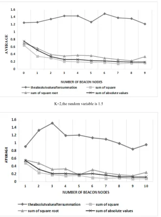
According to the simulation flow and the objective function in the last chapter, the number of unknown nodes is 5i (i = 1 ~ 10). When the values of k are 2, 3, 4, we calculate 50 sets of data and get the simulation results (Figure 5).
K=2,the random variable is 1.5
K=4,the random variable is 4 Fig. 5. Average error of node position
K=2,the random variable is 1.5
K=4, the random variable is 2 Fig. 6. Maximum error of node position
Conclusion: The sum of absolute values and the sum of square is most suitable for the objective function.
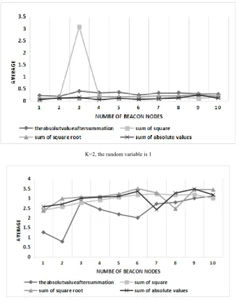
6.3 The calculation of k values
2 to 5, so in the optimization calculation, we first determine the optimal value of the initial calculation, while give the change interval of k is 2 to 5. As with the unknown node coordinates, we would like to know what is the relationship between the selec-tion of the objective funcselec-tion and the calculated value of k. Therefore, the following simulation experiment is to explore when the selection of different objective function, the variation of the calculated value of K with the increase of node number.
K=2, the random variable is 1
K=4,the random variable is 1.5
In the Figure 7, the maximum value of the calculated value of k is mostly above the true value. The sum of square root in the objective function fluctuates too violent-ly with respect to the sum of square and the sum of absolute values. Therefore, when select the objective function, the sum of square root is removed. While the sum of the absolute values and the sum of square are relatively stable, and the fluctuation range is smaller and better than the other objective function in the maximum value of the calculated value of k, so it is appropriate as the objective function.
Conclusion: The sum of the absolute values and the sum of the squares in the ob-jective function are suitable as the optimal obob-jective function, which is beneficial to the improvement of the path attenuation factor.
7
Conclusion
In this paper, we proposed a localization method for mobile robot nodes, and car-ried out the simulation experiment. In the simulation experiment, after selecting the objective function, the algorithm is optimized by the ranking method. The experi-mental results show that the proposed algorithm can achieve higher localization preci-sion in fewer nodes. In this paper, the environmental parameters, namely the path loss factor k, are calculated, and the calculated value of k is simulated and analyzed by using the optimized localization algorithm. At last, this paper compared the localiza-tion algorithm with the classical localizalocaliza-tion algorithm. The simulalocaliza-tion results show that the localization algorithm proposed in this paper has higher localization accuracy than the traditional classical localization algorithm when the number of nodes is larg-er than a clarg-ertain numblarg-er.
8
References
[1]Deshpande, N., Grant, E., & Henderson, T. C. (2014). Target localization and autonomous navigation using wireless sensor networks—A pseudogradient algorithm approach. IEEE Systems Journal, 8(1), 93-103. https://doi.org/10.1109/JSYST.2013.2260631
[2]Hu, Y., Ding, Y., Hao, K., Ren, L., & Han, H. (2014). An immune orthogonal learning particle swarm optimisation algorithm for routing recovery of wireless sensor networks with mobile sink. International Journal of Systems Science, 45(3), 337-350.
https://doi.org/10.1080/00207721.2012.723053
[3]Mahboubi, H., Moezzi, K., Aghdam, A. G., Sayrafian-Pour, K., & Marbukh, V. (2014). Distributed deployment algorithms for improved coverage in a network of wireless mobile sensors. IEEE Transactions on Industrial Informatics, 10(1), 163-174.
https://doi.org/10.1109/TII.2013.2280095
[4]Rawat, P., Singh, K. D., Chaouchi, H., & Bonnin, J. M. (2014). Wireless sensor networks: a survey on recent developments and potential synergies. The Journal of supercomputing, 68(1), 1-48. https://doi.org/10.1007/s11227-013-1021-9
[6]Tuna, G., Gungor, V. C., & Gulez, K. (2014). An autonomous wireless sensor network de-ployment system using mobile robots for human existence detection in case of disasters. Ad Hoc Networks, 13, 54-68. https://doi.org/10.1016/j.adhoc.2012.06.006
[7]Younis, M., Senturk, I. F., Akkaya, K., Lee, S., & Senel, F. (2014). Topology management techniques for tolerating node failures in wireless sensor networks: A survey. Computer Networks, 58, 254-283. https://doi.org/10.1016/j.comnet.2013.08.021
[8]Zhu, C., Shu, L., Hara, T., Wang, L., Nishio, S., & Yang, L. T. (2014). A survey on com-munication and data management issues in mobile sensor networks. Wireless Communica-tions and Mobile Computing, 14(1), 19-36. https://doi.org/10.1002/wcm.1219
9
Author
Peng An is Associate Professor at Ningbo University of Technology, Zhejiang, China ([email protected]).