Design and test of stem diameter inspection spherical robot
Longzhe Quan
1,
Ci Chen
2,
Yajun Li
1,
Yajing Qiao
1,
Dejun Xi
1,
Tianyu Zhang
3,
Wenfeng Sun
1* (1. College of Engineering, Northeast Agricultural University, Harbin 150030, China;2. College of Biosystems Engineering and Food Science, Zhejiang University, Hangzhou 310000, China;
3. State Key Laboratory of Robotics, Shenyang Institute of Automation, Chinese Academy of Sciences, Shenyang 110000, China)
Abstract: Stem diameter is an important parameter in the process of plant growth which can indicate the growth state and
moisture content of the plant, its automatic detection is necessary. Traditional devices have many drawbacks that limit their practical uses in general case. To solve those problems, a stem diameter inspection spherical robot was developed in this study. The particular mechanism of the robot has turned out to be suitable for performing monitoring tasks in greenhouse mainly due to its spherical shape, small size, low weight and traction system that do not produce soil compacting or erosion. The mechanical structure and hardware architecture of the spherical robot were described, the algorithm based on binocular stereo vision was developed to measure the stem diameter of the plant. The effectiveness of the prototype robot was confirmed by field experiments in a tomato greenhouse. The results showed that the machine measurement data was linearly correlated with the manual measurement data with R2 of 0.9503. There was no significant difference for each attribute
between machine measurement data and manual measurement data (sig>0.05). The results showed that this method was feasible for nondestructive testing of the stem diameter of greenhouse plants.
Keywords: stem diameter inspection, spherical robot, binocular stereo vision, Census transform
DOI: 10.25165/j.ijabe.20191202.4163
Citation: Quan L Z, Chen C, Li Y J, Qiao Y J, Xi D J, Zhang T Y, et al. Design and test of stem diameter inspection spherical robot. Int J Agric & Biol Eng, 2019; 12(2): 141–151.
1 Introduction
1In recent years, the development of agriculture, especially the greenhouse industry, has been paid more attention to the collection and monitoring of plant physiological information. The growth environment can be adjusted according to the growth condition of the plant. The growth states of plants after environmental changes can also be detected to make the regulation more scientific[1-4].
The stem diameter is an important parameter in plant growth which can indicate the growth state and moisture content of the plant[5,6].
Cultivation measures can be adjusted timely according to monitoring results, so the automatic monitoring of stem diameter is necessary.
At present, the main equipment to measure stem diameter is LDVT (Linear variable displacement transducer)[7]. However,
contact measurement not only need expensive devices, but also cause a negative effect on stem growth[8]. Thus LDVT has low
practicability in production. Compared with traditional methods, computer vision and image processing technology can achieve continuous, non-destructive, high accuracy, fast speed measurement. Those advantages make this technology has broad application prospects[9]. Among which binocular vision
Received date: 2018-01-31 Accepted date: 2019-03-12
Biographies: Longzhe Quan, PhD, Professor, research interests: intelligent agricultural equipment, Email: [email protected]; Ci Chen, MS candidate, research interests: agricultural robots and machine vision, Email: [email protected]; Yajun Li, MS candidate, research interests: agricultural mechanization engineering, Email: [email protected]; Yajing Qiao, MS candidate, research interests: agricultural mechanization engineering, Email: [email protected]; Dejun Xi, MS candidate, research interests: agricultural mechanization engineering, Email: [email protected]; Tianyu Zhang, PhD candidate, research interests: robot technology, Email: [email protected]. *Corresponding author: Wenfeng Sun, PhD, Professor, research interests: plant protection equipment. College of Engineering, Northeast Agricultural University, Harbin 150030, China. Tel: +86-451-55190997, Email: [email protected].
technology can obtain the plant growth parameters without using the calibration object which can achieve three-dimensional visualization measurement.
In the application of binocular vision technology, Takahashi et al.[10,11], Van Henten et al.[12], Xiang et al.[13] studied fruit
recognition and location. Meantime verify that its positioning accuracy can ensure the requirements of most picking operations. Rovira-Más et al.[14], Zhai et al.[15] studied the 3D reconstruction of
the 2D field operation map which is convenient to provide spatial information such as descriptions of surroundings for precision agriculture. Yang et al.[16], Huang et al.[17] studied binocular
vision used in obstacle detection, which can improve the safety and intelligence of the agricultural robots on the field of automatic navigation.
In order to reduce plant damage and work near the bottom of the plant, the camera with platform needs flexible operation in the greenhouse. Wheeled or tracked robots, traditionally used in agricultural working environment, will compact the ground and hinders the nutrient penetration, which can damage the plant and slow down the plant growing[18,19]. Thus, the spherical robot
which has compact structure, good dynamic and static balance, has been designed and tested as a low-cost robot that minimizes the damage to the plant while performing monitoring task. Robotic spheres are systems in which movements are induced by instability, so it is less invasive, causing minimum alterations on the soil. Considering their regular shape, this robot may recover easily from collisions. Besides, it can protect the binocular camera form hostile environment in the greenhouse because of its recoverable configuration. Several robotics spheres have been developed for quite different areas of applications. Bruhn et al.[20] and Michaud
et al.[21] have proposed spherical robot used for planetary
exploration. It also be used in the field of security, surveillance, inspection[22] and toy[23]. In the field of agricultural engineering,
friendly spherical mobile robot employed to monitor temperature and humidity in agricultural fields, which was used as a distributed sensor web.
Based on the concepts above, this study intends to develop and evaluate a flexible device for automatic measurement of stem diameter, in which spherical robot was used as the platform of binocular camera. In order to be better used in the greenhouse, several mechanical improvements were made. Firstly, a two-axis stable platform was made to reduce interference to the binocular camera caused by the rolling of the robot. Secondly, a rubber guide ring was designed to improve the stability of the robot. On this basis, the control system was constructed and an algorithm based on binocular vision was proposed to measure the stem diameter. Furthermore, to verify the validity of the developed spherical robot, a field experiments were performed.
2 Mechanical structure of spherical robot
A prototype model of the spherical robot was designed for both efficiency and cost effectiveness[24]. As shown in Figure 1, the
spherical robot was composed of four parts: motion system, control system, video acquisition system and energy system. The motion system includes spherical shell, rubber guide ring, DC motor, two-axis stable platform, servo motor, internal frame and balance weight. The control system includes slave controller, DC motor controller, servo motor controller, magnetic navigation sensor, gyroscope, photoelectric sensor module and Zigbee wireless serial port. The video acquisition system included binocular camera, wireless image transmission module and video acquisition card. The energy systems included batteries, transformer modules and
relays.
1. Spherical shell 2. Rubber guide ring 3. DC motor 4. Two-axis stable platform 5. Magnetic navigation sensor 6. Servo motor 7. Internal frame 8. Energy systems 9. Control system 10. Balance weight
Figure 1 Mechanical structure of stem diameters inspection spherical robot
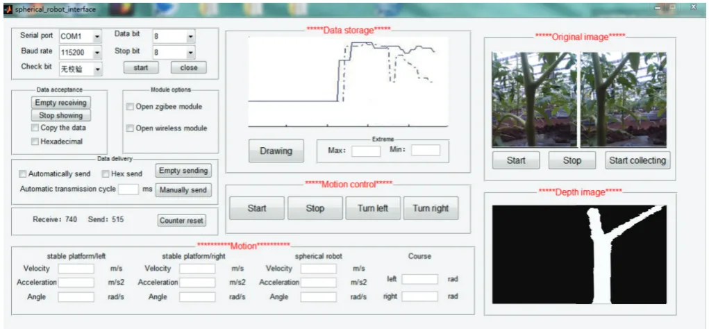
When the spherical robot works, the slave controller receives the host computer’s command and controls the DC motor to drive the counterweight away from the center of the spherical robot to give rise to self-motion. The magnetic tape was laid on the greenhouse pavement, and the magnetic navigation sensor received the magnetic signal from the tape in order to control the robot's course. The binocular camera was installed on the two-axis stable platform. When the plant passes, the photoelectric sensor sends the signal back to the host computer, the host computer receives the image and processes it. Finally, the stem diameter of the plant was calculated and displayed in the human-computer interaction interface, as shown in Figure 2.
Figure 2 Human-computer interface of control system
2.1 Introduction to two-axis stable platform
2.1.1 Structural design of stable platform
If the binocular camera was fixedly connected to the internal frame of the robot, the binocular camera would pitch and roll during movement of the spherical robot. This connection makes the images transmitted by binocular camera fluctuate greatly, which is inconvenient for later image processing. To solve this problem, a two-axis stable platform was designed. The platform isolate the motion of the robot from the binocular camera, creating a plane that remained horizontal in the robot, so the robot can better
track the target and return more accurate measurement data. The structural design of two-axis stable platform is shown in Figure 3.
binocular camera to rotate through the transmission of bevel gear1 and bevel gear 2 to realize the adjustment of the x direction. Servo motor 3 is fixed on the internal frame of the spherical robot by bolts, its output shaft is fixedly connected with gear 2, gear 2 mesh with gear 1, gear 1 and pitching rotation frame is fixedly connected, pitching rotation frame is connected with the camera fixed frame, and the camera fixed frame is fixed on the inner frame of the spherical robot. The servo motor 3 drives the pitching rotation frame rotating through the transmission of gear 1 and gear 2, and realizes the adjustment of the platform around the y direction. When the robot rolls along the y direction, gyroscope mounted on the two-axis stable platform measures the attitude and motion parameters of the platform, then provides feedback to the control system, control system controls servo motor 2 to rotate a particular angle, so that solve the problem that the camera rolled relative to the ground. When the robot pitches in the course of movement, the control system controls the servo motor 3 to rotate a particular angle to ensure that the camera axis is parallel to the ground, which solves the problem that the camera pitched relative to the ground.
1. Servo motor 2 2. Bevel gear 1 3. Bevel gear 2 4. Gear 1 5. Camera fixed frame 6. Turn lever 7. Pitching rotation frame 8. Gear 2 9. Servo
motor 3
Figure 3 Schematic diagram of two-axis stable platform 2.1.2 Performance analysis of stable platform
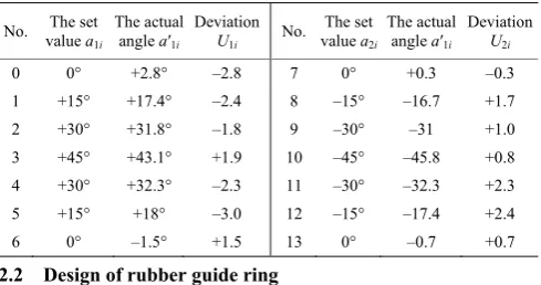
The isolation performance of two-axis stable platform was tested by swing test bench. Since the motion of x axis is the main source of interference, therefore, this experiment only tests the isolation of x-axis. The two-axis stable platform was fixed on the swing test bench, after the swing test bench start, the position instruction ai1was given in turn to rotate the measured axis.
Attach the mirror to the binocular camera and irradiate the mirror by a laser pointer. Then adjusted the position of the mirror to make the light beam be reflected on a preset coordinate paper. Besides, adjust the distance between the coordinate paper and the swing test bench, in order to make sure the light beam is reflected on the central region of the coordinate paper when the swing test bench was in horizontal position. Record the actual position of the binocular camera, and label it as a′1i . i was set to 0-6, and the
interval of degree is 15°. When the forward rotation is finished, conduct the reverse rotation experiment, and repeat the experiment.
U1i=a1i– a′1i U2i=a2i–a′2i
where, U1i is angular control accuracy when the measured axis was
in positive rotation; U2i is angular control accuracy when the
measured axis was in reverse rotation.
According to Table 1, when the swing test bench was set from
˗45° to +45°, angular position accuracy of two-axis stable platform always stay in the range of –3° to +3°. Due to the addition of
stem slant correction algorithm in the subsequent image processing, the error caused by rotating platform can be corrected. Therefore, the two-axis stable platform proposed in this paper is feasible to maintain camera attitude level.
Table 1 Angle error of two-axis stable platform
No. The set value a1i
The actual angle a′1i
Deviation
U1i No.
The set value a2i
The actual angle a′1i
Deviation
U2i
0 0° +2.8° –2.8 7 0° +0.3 –0.3
1 +15° +17.4° –2.4 8 –15° –16.7 +1.7
2 +30° +31.8° –1.8 9 –30° –31 +1.0
3 +45° +43.1° +1.9 10 –45° –45.8 +0.8
4 +30° +32.3° –2.3 11 –30° –32.3 +2.3
5 +15° +18° –3.0 12 –15° –17.4 +2.4
6 0° –1.5° +1.5 13 0° –0.7 +0.7
2.2 Design of rubber guide ring
When the spherical robot was used in greenhouse, it would yaw because of the bumpy road and uneven load of the robot. It is a great disturbance to the movement of the spherical robot, and put forward very high requirements to the design of control system. To solve this problem, a rubber guide ring was designed to enhance the anti-yawing performance of spherical robot and increase friction consequently.
Additional, in order to avoid abrasion caused by the contact between the spherical shell and the soil, the outer radius of the rubber guide ring was designed to be r+h. (r is radius of the spherical shell, h is soil sinkage).
From the Beck model[25], the relationship between the unit area
grounding pressure and the soil sinkage is:
( ) (Kc ) n
p h K h
b
= + ϕ (1)
where, p(h) is unit area grounding pressure, kPa; Kc is soil cohesive deformation modulus, kN/mn-1; K
φ is soil friction angle
deformation modulus, kN/mn; n is soil deformation index; h is soil
sinkage, m; b is width of the rubber guide ring, m.
The relationship between the unit area grounding pressure and the gravity of the spherical robot is:
( ) G p h
A
= (2)
where, G is gravity of the spherical robot, N; A is contact area of soil and rubber guide ring, m2.
Simplify the contact area to a rectangle, the length of the rectangle can be expressed as:
2 2
2 ( ) 2 2
L= × r h+ −r ≈ rh (3) Noting that:
A L b= × (4) Substituting Equation (2), Equation (3) and Equation (4) into Equation (1) with some algebraic manipulations, it follows:
( )
2 2
n c
G K
K h b
b× rh= + ϕ (5) The gravity of the spherical robot is 0.04 kN, the radius of the spherical shell is 0.15 m, the width of the rubber guide ring is 0.04 m, for greenhouse pavement, KC=0.95 kPa/mn-1, K
φ=
1528.43 kPa/mn, n=1.10, it can be obtained that h≈1 cm.
1.2-1.4[26], the value of L can be gotten by Equation (3), so we
obtained 0.076 m<Lb<0.092 m. Suppose Lb=0.09 m, so the installation position of the rubber guide ring is about 4.5 cm away from the center line of the spherical shell, as shown in Figure 4.
Figure 4 Design of rubber guide ring
3 Hardware architecture of spherical robot
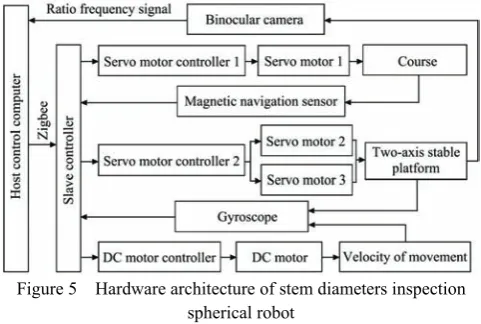
According to the task requirements and modular design idea of hardware architecture, the hardware architecture was designed as shown in Figure 5.
Figure 5 Hardware architecture of stem diameters inspection spherical robot
A mini PC with Intel Core (i7) 3.60GHz processor and 8.00G memory was selected as the host computer, which was responsible for collecting and processing image online and controlling the spherical robot’s motion. The SCM was chosen as the slave controller to control the two-axis stable platform, forward motion and navigation of robot. In view of the far distance between the host computer and slave controller and less amount of data, Zigbee module was chosen for communicating. It works in the 2400-2500 common frequency band, the transmission rate is up to 3300 bps, the transmission distance is up to 250 m.
The two-axis stable platform consisted of gyroscope, servo motor controller and servo motor. During movement of the spherical robot, slave controller triggered timer 0 interrupt in the design time, sent data request instruction through serial port. After receiving the command, the gyroscope returned the immediate status value including speed, acceleration and angle. The slave controller generated control parameters through a specific algorithm, and the control parameters were passed to the servo motor controller. The servo motor drove the platform to rotate around the x and y axis in opposite directions. The slave controller received the data returned by the gyroscope again after the timer was time out, the control parameters were generated again and sent to the servo controller. The process continues to constitute a servo system. The aim to control the two-axis stable platform was achieved.
In order to improve the real-time of navigation, we choose magnetic navigation instead of visual navigation which will take a lot of time because of complex calculations. This method is flexible, and convenient to change or expand the path at the same time[27]. Magnetic navigation sensor was mounted at the bottom
of internal frame of the spherical robot, and the magnetic tape was laid on the greenhouse pavement. When the sensor passed over the magnetic tape, the weak magnetic field above the magnetic tape can be detected, each sampling point on the sensor had a corresponding signal output. When the sensor detected the magnetic field, the output was high, otherwise, the output was low. These output signals were transmitted to the slave controller. The slave controller generated the control parameters and passed the parameters to the servo motor controller. The servo motor responsible for controlling the steering responded, adjusted to the direction of the spherical robot to make sure the spherical robot moves along the tape.
4 Visual system of spherical robot
4.1 Visual angle of binocular camera
As shown in Figures 6 and 7, it can be obtained by geometric relation:
2 tan 2 d
l′ = l β +B (6)
tan 2 d
R l
=
α
(7)
where, CL represents left camera of the binocular camera; CR represents right camera of the binocular camera; l′ represents coverage region of binocular camera field, cm; β represents horizontal visual angle of camera, deg; α represents vertical visual angle of camera, deg; B represents baseline distance between the left and right camera, cm; ld represents distance between the camera and the target, cm.
Figure 6 Horizontal visual angle of binocular camera
Figure 7 Vertical visual angle of binocular camera
4 3
=
β
α (8)
In order to ensure that two adjacent plants don’t appear in the view of camera at the same time, which will cause interference to subsequent image processing, l′ should be less than the distance between two adjacent plants. Generally, the distance between greenhouse plants is about 50 cm, so suppose l′=50 cm. Noting that baseline distance between the left and right camera in this paper is 4 cm, and the radius of the spherical robot is 15 cm. Bring the value into Equations (6)-(8), it can be obtained that the horizontal visual angle was about 98°, the vertical visual was about 74°, distance between the camera and the target was about 20 cm.
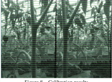
4.2 Camera calibration and binocular correction
Calibrating the camera is the precondition and guarantee of binocular depth measurement for the effect of calibration parameters on the future research in this field. For the binocular cameras, two cameras should be horizontal justification and each axis should be forward parallel, to get the calibration parameters and rectify the image so that the above requirement will be met. These camera parameters were determined by calibration procedure in MATLAB R2014a. The focal length, the center pixel of the image, the sizes of a pixel, and one parameter to compensate for any lens distortion are estimated by the procedure. In addition, the relative poses between the left and right images were also obtained through the calibration procedure.
Equipment required for camera calibration includes a binocular stereo vision camera (COMS, maximum resolution: 1280×960, baseline: 4 cm); a calibration plate (the distance of the near square center: 27 mm, the number of square: 8×8). The calibration results are shown in Table 2.
It can be seen from Table 2 that the focal length of the left and right camera is approximately equal. The optical center point coordinates in the near (640, 480), this is consistent with the parameters given by the manufacturer. The position relations of two cameras can be characterized by rotation matrix R and translation vector T, R and T are called camera external parameters.
It can be seen that the rotation matrix R is approximately the unit matrix from the binocular camera calibration results. It proves that the two cameras are forward parallel basically in physics. The baseline length which was obtained by calibration is 4.157037 cm, which is very close to the parameters provided by the manufacturer. Subsequently, the images were rectified using
intrinsic camera parameters. The aim of the image rectification was to make the optical axis parallel in the two cameras to process stereo matching and three-dimensional reconstruction. After rectification, the image rows of the same single point in the left and right image were unanimous.
Binocular rectification can be divided into two steps. Firstly, the plane of two cameras was re-projected, which requires the rotation matrix obtained by the above section of stereo calibration. Then, the left and right two planes were rotated by Equation (9) so that they can be kept exactly on the same plane.
1
1
l r
l r
R r r r r
−
⎧ = × ⎪
⎨ × =
⎪⎩ (9)
where, rl represents the rotation matrix required to achieve coplanarity for the left camera; rr represents the rotation matrix required to achieve coplanarity for the right camera.
The next step of binocular rectification is to make the left and right images rotate around their optical axes respectively, so that the ligature of main points of the two cameras is parallel to the pixel coordinate line, and the rotation matrix is shown as follows:
1 2 3 [ , , ] h
R = e e e (10)
where, 1 || || T e
T
= , 2 2 2
[ x, ,0]y
x y
T T e
T T
− =
+ , e3= ×e e1 2; Tx is the first value of the translation vector; Ty is the second value of the translation vector; ||T|| is the absolute value of translation vector.
After rectification, the images conform with the epipolar constraints[28], thus, in processing the stereo matching, we need
only to search its matching points on the same line, and the efficiency of the stereo matching is improved.
Figure 8 Calibration results
Table 2 Parameters of camera calibration
Camera Focal length Origin Distortion coefficient R T
Left [434.67, 473.91] [649.012, 491.646] [0.05572, –0.33415, –0.00248, 0.00154, 0]
1.0000 0.0027 0.0002 0.0027 0.9999 0.0125 0.0001 0.0125 0.9999
R
⎡ ⎤
⎢ ⎥
= −⎢ ⎥
⎢− − ⎥
⎣ ⎦
41.57037 1.55634
6.08450
T −
⎡ ⎤
⎢ ⎥
= ⎢ ⎥
⎢− ⎥
⎣ ⎦
Right [435.52, 473.42] [655.952, 501.398] [0.03185, –0.11786, –0.00047, –0.00060,0]
4.3 Stereo Matching
Stereo matching is the most important link within the overall system, which is to gain 3D information by looking for the characteristic points and calculating its disparity between the two correct images.
To reduce the computation cost, greyscale images were selected for the subsequent image processing. Since the collected original images are stored according to the RGB color model, to preserve the true nature of the plant, the original image was transformed from RGB space to gray space by weighted gray method, the greyscale can be calculated by Equation (11).
f(x,y)=0.3Red(x,y)+0.59Green(x,y)+0.11Blue(x,y) (11) where, f(x,y) is the gray values of the pixel; Red(x,y) is red chromatic values of the pixel; Green(x, y) is green chromatic values of the pixel; Blue(x, y) is blue chromatic values of the pixel.
In order to minimize the influence produced by the changing illumination on the image, the Rank transformation of greyscale was selected to be matching element, which is an non-parametric technique based on a mathematical statistical method and is validated to be sufficiency robust against image distortion and noise[29].
the center, a rectangle area was taken as the Rank window. The number of neighbor pixel in Rank window was counted as the value of the Rank transformation whose grayscale was smaller than that of the center point, as given by Equation (12).
( , )
2 1 1 2
2 1
( , ) ( ( , ), ( , ))
1 ( , )
0
r x y f x y f x y
x x
x x
x x
⎧ = + +
⎪
⎨ =⎧ <
⎪ ⎨ ≥
⎩ ⎩
∑
ζ ηδ ζ ηδ (12)
where, r(x,y) is the Rank transformation value of target pixel; ζ, η
are the sizes of the Rank window, pixel; f(x+ζ, y+η) is the greyscale of neighbor point; δ(x1,x2) is a sign function.
If the two points in the left and right images are correctly matched, the corresponding pixels in the neighborhood should also be correctly matched. Therefore, in the matching process, the neighborhood similarity is usually used as the basis of matching. SAD (sum of absolute differences) was used as the fastest algorithm. A fixed-sized SAD window was moved to the center of the reference point and matching point. Thus, the optimal disparity was measured by the distance between the most similar matching pairs, as given by Equation (13).
,
( , , ) ( , ) ( , )
SAD R L
W
C x y k r x y r x k y
∈
=
∑
+ + − + + +ζ η
ζ η ζ η (13)
where, CSAD is the matching cost, which measures the difference in corresponding points; k is the matching distance, pixel; rL is the Rank transform value of the reference point; rR is the Rank transformation value of the matching point; W is matching window.
When CSAD is the minimum, the best matching between left and right images is achieved, the disparity at this time is:
arg min SAD( , , ) k
d= C x y k (14)
Generally, there are some erroneous matches after stereo matching. To enhance the accuracy of disparities obtained, false matches should be rejected. The Census transform was performed on the Rank window, as given by Equation (15).
( , )
( , ) ( ( , ), ( , ))
R x y =BitStringζ ηδ f x y f x+ζ y+η (15)
where, R(x,y) is the Census transformation value; Bitstring represents linking the front and back of the Rank value.
Define distance of HAMMING between RR(x1,y1)and
RL(x2,y2)as follows:
2 2 1 1
( , ) 2 2 2 2 1 1 1 1
( ( , ), ( , ))
( ( , ), ( , )) ( ( , ), ( , ))
R L
R L
HAMMING R x y R x y
f x y f x y f x y f x y
=
+ + ⊕ + +
∑
ζ ηδ ζ η δ ξ η(16) The HAMMING distance between two pixels of the same relative position of the matching window was calculated, and the sum was also calculated. Also, the constraint function of the algorithm can be obtained, as given by Equation (17).
( , , ) ( , )
( ( , ), ( , ))
m n
r l
g x y k HAMMING
R x m y n R x m k y n
= Σ
+ + + + + (17)
where, g(x,y,k) is constraint function; m, n are the sizes of the matching window.
When there are multiple optimal values, the Equation (17) can be used as a constraint. Take the smallest pixel pair of g(x,y,k) as the best match, then k at this point is the disparity of the corresponding points, which can also be represented as d.
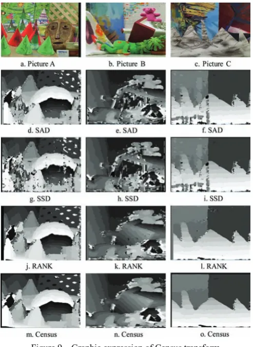
The paper uses images A B and C to test the Census transform and compares it with traditional SAD, SSD and RANK transformation. The parallax effect is shown in the Figure 9, where Figures 9a-9c is the left figure of the test images, 9d-9f is the parallax figure obtained by SAD algorithm, 9g-9i is the parallax
figure obtained by SSD algorithm, 9j-9l is the parallax figure obtained by RANK transformation, and 9m-9o is the parallax figure obtained by census transformation. By comparing the parallax graphs obtained by the four algorithms, it can be found that, the parallax map obtained by the census stereo matching algorithm adopted in this paper is more clear at the edge and contour of the image and other features. There are fewer white areas caused by wrong matching, which can effectively improve the accuracy of subsequent calculation.
Figure 9 Graphic expression of Census transform
4.4 Calculation of stem diameter
Because the binocular camera used in this application is integrated with two parallel uniform monocular cameras, the 3D coordinates of matching pairs can be calculated based on disparities, as shown in Figure 10. There are three coordinates, including device coordinate system oxy, image coordinate system ouv, left camera coordinate system OXYZ. From the similarity of the triangle it can be obtained that:
( L R)
P
P P L R
B x x B fB
Z
Z f Z x x
− − = ⇒ =
− − (18a)
P L
P X
x f
Z
= (18b)
P L
P Y
y f
Z
= (18c)
Figure 10 Binocular stereo vision model Noting that:
L R
d=x −x (19) Using Equation (18a) and Equation (18b) as well as Equation (19), the abscissa of the target point under left camera coordinate can be obtained:
L P
B x X
d
⋅
= (20a)
Also, according to Equations (18a), (18c) and (19), the ordinate of the target point under left camera coordinate can be obtained:
L P
B y Y
d
⋅
= (20b)
The relationship between the image coordinate system and device coordinate system can be expressed as Equations (21a) and (21b):
0 L L
x
u u
s
= + (21a)
0 L L
y
v v
s
= + (21b)
where, s is the pixel size of the image, mm/pixel; (u0,v0) is the
origin in the left image under image coordinate system; uL is the abscissa of the target point in the left image under image coordinate system; vL is the ordinate of the target point in the left image under image coordinate system.
Combine Equations (20a) and (21a), it can be obtained:
P ( L 0) B
X u u s
d
= − (22a)
Likewise, it can be obtained:
0
( )
P L
B
Y v v s
d
= − (22b)
Equation (22b) can be rewritten as:
0 P L
Y d
v v
B s
⋅
= +
⋅ (23)
In the above equation, B, (u0,v0), s can be obtained from camera calibration, d can be obtained from stereo matching. Therefore, the coordinates of the target point in the left camera coordinate system can be obtained only if we know the pixel coordinate of the target point in the image coordinate system.
Based on the above principle, we give the procedure to calculate stem diameter as follows:
1) Perform an adaptive threshold operation on the parallax map, in which the pixel of stem part was set to 255 and the rest to 0.
2) Perform the morphological closure on the image to eliminates holes and smooth edge.
Because of the uncertainty of plant growth and the error of
two-axis stable platform, the upright posture of the tomato stalks captured by the binocular camera can’t be guaranteed. In order to measure the diameter of the stem at the bottom of the tomato more accurately, the tomato stalks need to be vertically corrected, the steps of tilt correction are as follows:
1) Perform edge detection on the processed parallax map. 2) Perform the Progressive Probabilistic Hough Transform, set up a dynamic threshold varying from large to small to improve the detection accuracy.
3) Average the inclination angle of each line to get a better spin effect.
4) Apply affine transformation to images and cut the image to the right size.
The correction process was shown in the Figure 11.
a. Pretreatment b. Edge detection
c. PPHP d. Affine transformation Figure 11 Vertical alignment of tilt stem
After tilt correction, we can obtain the diameter of stem from the following steps:
1) For the processed parallax figure, as shown in Figure 12, search line by line from the bottom of the image, find the abscissa ui1, whose left adjacent pixel’s value is 0 and right adjacent pixel’s value is 255. Then find the abscissa ui2, whose left adjacent pixel’s value is 255 and right adjacent pixel’s value is 0. If two satisfying coordinates are found in a row, which means the stem branch is searched, stop search and note the ordinate of this row to be vi.
2) Suppose the ordinate of the stem branch, which can be obtained from Equation (22b), to be Yi. In addition, Y1, Y2 and Y3
express the ordinate of the three measured position under left camera coordinate system, among which Y1=Yi–5 cm, Y2=Yi–7.5 cm,
Y3=Yi–10 cm, then we can achieve the ordinate of measured
position under coordinate from Equation (23), suppose them to be v1, v2 and v3.
3) When the ordinate is v1, find the abscissa u11, whose left
adjacent pixel’s value is 0 and right adjacent pixel’s value is 255, next, find the abscissa u12, whose left adjacent pixel’s value is 255
and the right adjacent pixel’s value is 0.
4) Find out the disparity values d11 and d12corresponding to
u11 and u12, then the abscissa of these pixel under left camera
11 11 11
( o) B
X u u s
d
= − (24a)
12 12
12
( o) B
X u u s
d
= − (24b)
Therefore the stem diameter of measurement position 1 can be calculated from Equation (25):
D1=X12– X11 (25)
5) Then, calculate the stem diameter of measurement position 2 and 3 in the same method.
The captured images were transmitted by the wireless graph transmission module and they were transmitted by the analog video signal. The transmission frequency is 2300-2600 mHz and the output power is 800 MW with no delay in theory. During the
matching process, the size of the Rank transform window was 5×5 pixels, the size of the matching window was 9×9 pixels. The minimum disparity was set to 0. Complete the match by sliding the SAD window, for each target point in the left image, search the right image to find the best match. The corrected images were aligned strictly in each line in the experiment. We can reduce the number of disparity by limiting the search range of the matching point, thus the calculation time can be shortened. Twenty images of 1280×960 pixels were selected for time testing, and the time was shown in Table 3. The average time was about 3.15 s. The distance between two adjacent plants was 50 cm, so the movement speed of the spherical robot should be set to 0.16 m/s. The diameter of the spherical robot is 30 cm, and the angular velocity of the spherical robot is 0.17 r/s (1.07 rad/s).
Figure 12 Vertical alignment of tilt stem
Table 3 Image processing time
Plant 1 2 3 4 5 6 7 8 9 10
Time 3.1644 3.1450 3.1651 3.1088 3.1309 3.1380 3.1162 3.1181 3.1267 3.1199 Plant 11 12 13 14 15 16 17 18 19 20 Time 3.1443 3.1377 3.0908 3.1018 3.1078 3.0653 3.0699 3.6901 3.0844 3.1042
5 Experiment results
5.1 Materials and methods
The prototype of spherical robot was built up. Camera calibration was carried out in MATLAB R2017b. Implementations of binocular correction, stereo matching and stem diameter calculation were developed using the OpenCV Library under the VS2013 environment.
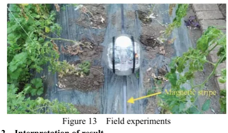
To further verify the feasibility of spherical robot, field tests were carried out in the greenhouse of Tomato in the college of Agriculture of Northeast Agricultural University. The test object were 20 tomatoes at the beginning of the fruit period (the breed is Maofen 803). To ensure good illumination conditions and image quality, the test was conducted under clear weather conditions. The experimental process was shown in Figure 13.
Two rows of tomatoes were selected and each row had ten plants. When the experiment began, recorded the data measured by robot in sequence. When the tenth tomato was detected in the row, then was changed to the other row. When the task has finished, the manual measurement was carried out. We measure the diameter of 5 cm, 7.5 cm and 10 cm below the branch with a
vernier caliper. For each position of one plant, measured three times and took the mean value as the manual measurement value. Figure 14 shows the image processing results of 20 stalks.
Figure 13 Field experiments
5.2 Interpretation of result
Figure 14 Image processing result
Table 4 Measured results of machine and manual
No. Monitoring site/cm
Manual measurement
value
Machine measurement
value
Deviation Fractional error No.
Monitoring site/cm
Manual measurement
value
Machine measurement
value
Deviation Fractional error
Plant 1
5 6.54 6.74 0.20 3.06%
Plant 11
5 7.33 7.22 –0.11 –1.50%
7.5 5.91 6.08 0.17 2.88% 7.5 6.97 6.79 –0.18 –2.58%
10 6.44 6.62 0.18 2.80% 10 7.24 7.16 –0.08 –1.10%
Plant 2
5 5.83 5.69 –0.14 –2.40%
Plant 12
5 7.46 7.66 0.20 2.68%
7.5 4.87 5.18 0.31 6.37% 7.5 6.59 6.71 0.12 1.82%
10 5.46 5.58 0.12 2.20% 10 6.69 6.91 0.22 3.29%
Plant 3
5 6.24 6.34 0.10 1.60%
Plant 13
5 7.23 7.32 0.09 1.24%
7.5 5.75 5.74 –0.01 –0.17% 7.5 6.20 6.36 0.16 2.58%
10 5.80 5.76 –0.04 –0.69% 10 6.37 6.38 0.01 0.16%
Plant 4
5 7.24 7.62 0.38 5.25%
Plant 14
5 6.86 6.92 0.06 0.87%
7.5 5.50 5.34 –0.16 –2.91% 7.5 6.62 6.85 0.23 3.47%
10 6.04 6.51 0.47 7.78% 10 6.52 6.86 0.34 5.21%
Plant 5
5 7.15 7.02 –0.13 –1.82%
Plant 15
5 7.09 7.28 0.19 2.68%
7.5 5.30 5.19 –0.11 –2.08% 7.5 6.66 6.84 0.18 2.70%
10 6.17 6.01 –0.16 –2.59% 10 6.87 6.97 0.10 1.46%
Plant 6
5 6.02 5.91 –0.11 –1.83%
Plant 16
5 6.79 6.81 0.02 0.29%
7.5 5.04 5.17 0.13 2.58% 7.5 5.42 5.65 0.23 4.24%
10 5.38 5.61 0.23 4.28% 10 5.50 5.37 –0.13 –2.36%
Plant 7
5 7.23 7.13 –0.10 –1.38%
Plant 17
5 7.22 7.30 0.08 1.11%
7.5 5.11 5.12 0.01 0.20% 7.5 6.76 6.53 –0.23 –3.40%
10 6.06 5.92 –0.14 –2.31% 10 6.85 6.79 –0.06 –0.88%
Plant 8
5 6.05 6.15 0.10 1.65%
Plant 18
5 6.20 6.28 0.08 1.29%
7.5 4.91 4.75 –0.16 –3.26% 7.5 5.51 5.42 –0.09 –1.63%
10 6.03 5.91 –0.12 –1.99% 10 5.90 6.02 0.12 2.03%
Plant 9
5 7.24 7.17 –0.07 –0.97%
Plant 19
5 6.80 6.98 0.18 2.65%
7.5 6.17 6.26 0.09 1.46% 7.5 5.28 5.38 0.10 1.89%
10 6.72 6.68 –0.04 –0.60% 10 5.86 6.10 0.24 4.10%
Plant 10
5 6.75 6.84 0.09 1.33%
Plant 20
5 6.84 6.96 0.12 1.75%
7.5 5.86 5.77 –0.09 –1.54% 7.5 5.40 5.31 –0.09 –1.67%
Figure 15 Regression analysis
For some points with larger deviations, the cause may be: 1) The spherical robot is in motion, two-axis stable platform response delay, and the camera cannot keep the stable attitude in real time.
2) Error in internal and external parameter correction of binocular camera. 3) Inaccurate stereo matching. 4) Error of manual measurement.
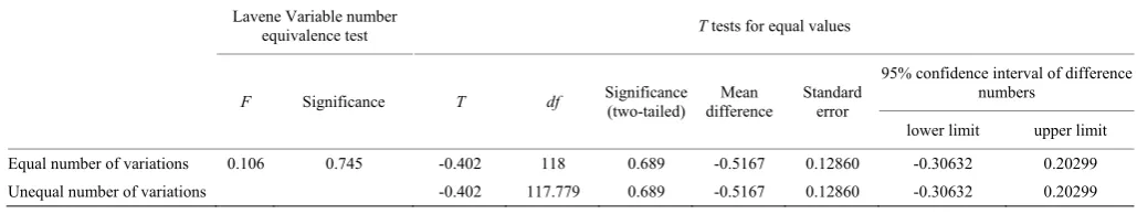
To test whether the machine measurement can be applied to the practical application, a significant test on the result of machine measurement and the manual measurement value was carried out. T-test was used as the test method. From Table 5, we can find that in the homogeneity test of variance in Levene’s, sig=0.745 > 0.05, the original hypothesis was accepted. So we use the T-test results with the same variance, that is sig′=0.689>0.05. Acknowledges the original hypothesis that there is no significant difference between the two groups of data. According to the results of T-test, there is no significant difference between manual measurement value and machine measurement value which can prove the method developed in this paper has high reliability and lower cost.
Table 5 Significance test
Lavene Variable number
equivalence test T tests for equal values
F Significance T df Significance
(two-tailed)
Mean difference
Standard error
95% confidence interval of difference numbers
lower limit upper limit Equal number of variations 0.106 0.745 -0.402 118 0.689 -0.5167 0.12860 -0.30632 0.20299 Unequal number of variations -0.402 117.779 0.689 -0.5167 0.12860 -0.30632 0.20299
6 Conclusions
A spherical robot was developed and used to monitor the stem diameters of greenhouse plant, which was nondestructive and fast with no calibrated objects. Considering it is used in greenhouse, there are several improvements to the traditional spherical robot: a two-axis stable platform designed to reduce the interference caused by the rolling of the spherical robot to the binocular camera; the rubber guide ring was developed to improve the stability of the spherical robot. Based on the binocular vision, an algorithm for measuring the stem diameter of the plant was proposed, and the measurement accuracy was tested by field experiment. The results showed that the machine measurement value has good linear correlation with manual measurement value. On this basis, a significance test between manual measurement and machine measurement value were conducted, its result shows there is no significant difference between the two groups. This paper provides a new idea for monitoring stem diameter of greenhouse plants with short plant size and less branching. It has a significance for improving plant cultivation and management.
Acknowledgements
The authors gratefully thank the financial support provided by the National Key Research and Development Program of China(2018YFD020080709), the Fund for the Returned Overseas Chinese Scholars of Heilongjiang Province(LC2018019) and Academic Backbone Foundation of NEAU(17XG01).
[References]
[1] Trejo-Perea M, Herrera-Ruiz G, Rios-Moreno J, Castaneda Miranda R, Rivas-Araiza E. Greenhouse energy consumption prediction using neural networks models. Int J Agric & Biol Eng, 2009; 11(1): 1–6.
[2] Campillo C, Garcia M I, Daza C, Prieto M H. Study of a non-destructive method for estimating the leaf area index in vegetable crops using digital images. Hortscience, 2010; 45(10): 1459–63.
[3] Hwang J, Shin C, Yoe H. Study on an agricultural environment monitoring server system using wireless sensor networks. Sensors, 2010; 10(12): 11189–11211.
[4] Jesus Roldan J, Joossen G, Sanz D, del Cerro J, Barrientos A. Mini-UAV based sensory system for measuring environmental variables in greenhouses. Sensors, 2015; 15(2): 3334–3350.
[5] Gallardo M, Thompson R B, Valdez L C, Fernandez M D. Use of stem diameter variations to detect plant water stress in tomato. Irrigation Science, 2006; 24(4): 241–55.
[6] Meng Z, Duan A, Liu J, Zhang J. Advances on diagnosis of crop moisture content from changes in stem diameters of plants. Transactions of the CSAE, 2005; 21(2): 30–33. (in Chinese)
[7] Intrigliolo D S, Castel J R. Continuous measurement of plant and soil water status for irrigation scheduling in plum. Irrigation Science, 2004; 23(2): 93–102.
[8] Stao N, Hasegawa K. A computer controlled irrigation system for muskmelon using stem diameter sensor. Acta Horticulturae, 1995; 226: 91–98.
[9] Ying Y B, Fu B Z, Jiang Y Y, Zhao Y. Application of machine vision technique to automation of agricultural production. Transactions of the CSAE, 1999; 15(3): 199–203.(in Chinese)
[10] Takahashi T, Zhang S, Fukuchi H. Binocular stereo vision system for measuring distance of apples in orchard (Part 1) – Method due to composition of left and right images. Journal of the Japanese Society of Agricultural Machinery, 2000; 62(1): 89–99.
[11] Takahashi T, Zhang S, Fukuchi H. Binocular stereo vision system for measuring distance of apples in orchard (Part 2) – Analysis of and solution to the correspondence problem. Journal of the Japanese Society of Agricultural Machinery, 2000; 62(3): 94–102.
[12] Van Henten E J, Hemming J, Van Tuijl B A J. An autonomous robot for harvesting cucumbers in greenhouse. Autonomous Robots, 2002; 13: 241–258.
[13] Xiang R, Ying Y B, Jiang H Y, Peng Y S. Localization of tomatoes based on binocular stereo vision. Transactions of the CSAE, 2012; 28(5): 161–167.(in Chinese)
[14] Rovira-Más F, Zhang Q, Reid F. Stereo vision threedimensional terrain maps for precision agriculture. Computers and Electronics in Agriculture, 2008;60(2): 133-143.
method of various obstacles in farmland based on stereo vision technology. Transactions of the CSAM, 2012; 28(5): 161–167.(in Chinese)
[17] Huang Y, Young K. Binocular image sequence analysis: Integration of stereo disparity and optic flow for improved obstacle detection and tracking. EURASIP Journal on Advances in Signal Processing, 2008; 843232. https://doi.org/10.1155/2008/843232.
[18] Hernandez J D, Barrientos J, del Cerro J, Barrientos A, Sanz D. Moisture measurement in crops using spherical robots. Industrial Robot-an International Journal, 2013; 40(1): 59–66.
[19] Cancar L, Sanz D, Hernandez J D, del Cerro J, Barrientos A. Precision humidity and temperature measuring in farming using newer ground mobile robots. Springer International Publishing, 2014-06-15
[20] Bruhn F C, Kratz H, Warell J, Lagerkvist C-I, Kaznov V, Jones J A, et al. A preliminary design for a spherical inflatable microrover for planetary exploration. Acta Astronautica, 2008; 63(5-6): 618–31.
[21] Michaud F, Lafontaine J D, Caron S A. Spherical robot for planetary surface exploration. Proceeding of the 6th International Symposium on Artificial Intelligence and Robotics & Automation in Space, 2001. [22] Seeman M, Broxvall M, Saffiotti A, Wide P. An autonomous spherical
robot for security tasks. Proceedings of the 2006 IEEE International
Conference on Computational Intelligence for Homeland Security and Personal Safety, 2006; pp.51–55.
[23] Michaud F, Caron S. Roball, the Rolling Robot. Autonomous Robots, 2002; 12(2): 211–222
[24] Quan L Z, Chen C, Zhang T Y, Qiao Y J. A Spherical robot with obstacle avoidance function for crop bottom stem inspection. China Patent, ZL201610383579.3. 2016-06-0.
[25] Bekker G. Introduction to terrain-vehicle systems. Ann Arbor: University of Michigan Press, 1969.
[26] Geng R Y, Zhang D L, Wang X Y, Yang Z D. New agricultural mechanics. Beijing: National Defense Industry Press, 2015.(in Chinese) [27] Zhou C D. Research on the key technologies of magnetic guided
automated guided vehicle and applications. PhD dissertation. Nanjing: Nanjing University of Aeronautics and Astronautics, 2012. (in Chinese) [28] Brown M Z, Burschka D, Hager G D. Advances in computational stereo.
IEEE Transactions on Pattern Analysis and Machine Intelligence, 2003; 25(8): 993–1008.