Localization and controlling the mobile robot by sensory data fusion
Saeed Erfani
*, Ali Jafari, Ali Hajiahmad
(Department of Agricultural Machinery Engineering, College of Agriculture and Natural Resources, University of Tehran, Karaj, Iran)
Abstract: Localization of a mobile robot with any structure, work space and task is one of the most fundamental issues in the field of robotics and the prerequisite for moving any mobile robot that has always been a challenge for researchers. In this paper, Dempster-Shafer (D.S.) and Kalman filter (K.F.) methods are used as the two main tools for the integration and processing of sensor data in robot localization to achieve the best estimate of positioning according to the unsteady environmental conditions and a framework for Global Positioning System (GPS) and Inertial Measurement Unit (IMU) sensor data fusion. Also, by providing a new method, the initial weighing on each of these GPS sensors and wheel encoders is done based on the reliability of each one. The methods were compared with the simulation model and the best method was chosen in each situation. In addition to obtaining the geometric equations governing the robot, a Proportional Integral Derivative (PID) controller was used for the kinematic control of the robot and implemented in the MATLAB Simulink. Also, using these two Mean Absolute Deviation (MAD) and Mean Square Error (MSE) criteria, the localization error was compared in both K.F. and D.S. methods. In normal Gaussian noise, the K.F. with a mean error of 2.59% performed better than the D.S. method with a 3.12% error. However, in terms of non-Gaussian noise exposure, which we are faced with in real condition, K.F. information was associated with a moderate error of 1.4, while the D.S. behavior in the face of these conditions was not significantly changed.
Keywords: sensory data fusion, mobile robot, localization, Dempster-Shafer method, Kalman filter
Citation: Erfani, S., A. Jafari, and A. Hajiahmad. 2019. Localization and controlling the mobile robot by sensory data fusion. Agricultural Engineering International: CIGR Journal, 21(2): 86–97.
1 Introduction
Currently, agricultural automation is inevitable in
order to save on costs and produce more per unit area.
Robotics can also meet the goals of automation in
agriculture, by minimizing the tough, risky, deadly and
long working conditions, along with precise monitoring
and control. Between 1750 and 1900, a revolution in the
agricultural industry was formed at the same time as
fundamental changes in American agriculture. The basis
of this revolution was the entry of machines in the
industry. The idea of self-driving agricultural vehicles is
not very new, and the prototype of a non-driver
agricultural tractor, controlled through a cable, dates back
to the 1960s (Roberts et al., 1998). In the 1980s, with the
Received date: 2018-04-26 Accepted date: 2019-01-20
∗ Corresponding author: Saeed Erfani, Ph.D. Student, Department of Agricultural Machinery Engineering, College of Agriculture and Natural Resources, University of Tehran, Karaj, Iran. Tel: +98 2632248085, Email: int.utcan@ut.ac.ir
development of computer science and the ability to use
sight sensors, they created new situations for
self-contained robots, which were first used by
researchers at the University of Michigan and the
University of Texas. In the decade for the first time, an
orange harvesting robot was designed and developed by
researchers at the University of Florida (Edan, 1995).
With the development of research in this field and the
development of tools used to guide robots, including
optical, ultrasound and radio sensors, the problem of
increasing the accuracy and speed of the robots was
considered (Murakami et al., 2006). Data fusion is a
method for combining the data from several sources of
information used to obtain a brighter picture of the
problem being investigated and measured. Data fusion
systems are currently being used in a variety of fields,
including sensor networks, robotics, photo and video
processing, and smart system design. A lot of researches,
especially in recent years, has been done in the field of
intelligent systems in this area with the ability of
organisms, especially the ability of the human brain (Hall
and Llinas, 1997). Klein (1993) provided a definition of
the integration of sensor data, which combines sensor
data, from one type to different sources of data. Both
definitions provide a general form in the use of sensors
and can be used in a variety of applications, including
remote sensing. The authors have reviewed many of the
methods of data fusion and discussed each one. Based on
the strengths and weaknesses of previous work, a basic
definition of information integration is presented as
follows: information integration is an effective way to
automatically or semi-automatic conversion of
information from different sources or at different time
points into an effective output that in the decision-making
process, acts automatically or supports human
decision-making. In their research, the neural network
tool is used in data fusion and describes different levels of
data fusion. Ghahroudi and Fasih (2007) have used the
fusion of sensor data by using fuzzy logic utilization at
the decision level in the driver assistance system.
Subramanian et al.(2009) used a combination of optical
and visual sensors via a fuzzy system to auto routing
agricultural vehicles in specific routes of citrus orchards,
where the routing error improved in comparison with the
use of separate sensors. In this research, the results of the
data fusion prior to the decision were refined by the
Kalman filter. Akhoundi and Valavi (2010) used fuzzy
systems to integrate sensor data and showed that
aggregation of sensor data by this method is more
efficient than the sum of sensor data separately. This
fuzzy system included a fuzzy rule base based on sensors
that were complementary in accuracy and bandwidth. In
studies for localization, the combination of the global
positioning system and other sensors such as inertial
measurement sensors, position detection sensors (digital
compass), camera, radar and laser sensors, have shown
more accurate results than the use of only the global
positioning system (GPS) (Keicher and Seufert, 2000;
Subramanian et al., 2006; Li et al., 2010). In numerous
studies, differential global positioning system (DGPS)
has been used to determine the position with a precision
of a few centimeters in agricultural conditions. The
combination of GPS speed with the inertial navigation
systems (INS) sensor was used to measure the slip angle
of the vehicle and the tire when it was turned (Bevly et al.,
2001). In other research, Zhang et al. (2002) equipped an
agricultural tractor with an intelligent navigation system
with machine vision sensors and optical fiber gyroscope.
The results of this assessment showed that the intelligent
navigation system, combined with several navigation
sensors, could drive agricultural machinery in the field of
row crop without crossing the product. Also, Nagasaka et
al. (2004) used this navigation system for automatic
transplantation in rice fields. Their experiments showed
that the precision of folding with this method was
favorable, but it was not sufficiently accurate for spraying
and mechanical weeding operations because of the
movement among the rows. In a research conducted by
Mizushima et al. (2011) positioning sensors were
combined with three vibrational gyroscopes and two
inclinometers. Park (2016) for safe and comfortable
mobile robot navigation in dynamic and uncertain
environments, extended the state of the art in analytic
control of mobile robots, sampling based optimal path
planning, and stochastic model predictive control. Self
locating method was used based on fuzzy three
dimensional grid by Shi et al. (2017), in which, with
reduced computing, accuracy was increased.
Shafer (1976) introduced the theory of evidence, later
known as the Dempster-Shefer theory. The basis of this
approach is to integrate data into evidence or beliefs that
can manage information deficiencies. This was a
reinterpretation of Arthur Dempster's research in the
1960s, which, according to Dempster, has been largely
modified by Shafer (Shafer et al., 2003).
The Dempster-Shafer theory is a generalization of
Bayesian theory, widely used in computer science and
artificial intelligence, and resembles fuzzy sets
(Rakowsky, 2007). These three aforementioned theories
and the capabilities of each one are compared widely in
the sensor data fusion, and in some applications, the
Dempster-Shafer theory is used to link other data fusion
methods (Betz et al., 1989; Boston, 2000; Fenton et al.,
1998; Murphy, 1998; Pagac et al., 1998). Denoeux et al.
(2018), provided two new division methods, along with
simulation of some applications in the Dempster method.
weighting method in Dempster-Shafer theory by a fuzzy
algorithm that could use the evidence obtained from
different methods to classify the target.
Despite extensive research in the field of robotics and
control, the implementation of plans and methods of
localization in the agricultural industry have been less
studied due to the fundamental difference in the
laboratory environment with real conditions. Because
highly accurate sensors such as DGPS, in addition to the
high cost, have access restrictions, In this paper, various
methods of integrating global positioning unit and inertia
measurement unit are utilized by Dempster-Shafer theory
as well as Kalman filtering, and the results were
compared to select an accurate method for localization at
an appropriate cost. Also, by introducing a new method,
initial weighting has been made on the information of
each of the GPS sensors and wheel encoders, based on
the reliability of each one. In addition to obtaining the
geometric equations governing the robot, a Proportional
Integral Derivative (PID) controller was implemented in
the MATLAB Simulink for kinematic control and
evaluation of the robot localization algorithms.
The rest of the paper is organized as follows: the
kinematic modeling of the agricultural robot, the
simulation of the robot in the MATLAB SimMechanic,
the control of the robot with its results and localization by
Dempster- Shafer (D.S.) and Kalman filter (K.F.) are
given in Materials and method section. Comparing of
these two methods and the results is presented in Result
and discussions. Finally, some conclusions are
highlighted.
2 Materials and methods
2.1 Modeling
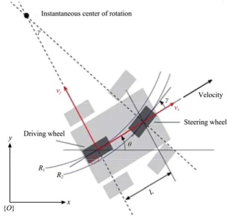
In this section, a model will be created for a robot that
is a car-like robot. The typical model for the four-wheel
robots is the bicycle model shown in Figure 1. The
two-wheel drive model has a rear wheel mounted on its
body, and the front wheel plate rotates around a vertical
axis for steering. The position of the robot is represented
by a moving coordinate system whose x-axis is in the
direction of moving forward of the robot and its center
corresponds to the center of the rear axle of the robot. The
configuration of the robot is also defined by general
coordinates q=(x,y,θ)∈C in which, C, is an Euclidean
two-dimensional space. In this coordinate system, the speed of the robot is along the x-axis, because the robot
cannot slip sideways. Because of the low speed,
longitudinal slip and centrifugal force can be ignored.
vx=v, vy=0 (1)
The wheels cannot move in the direction of the dashes,
and these two dashes cut off at one point, which is called
the instantaneous center of rotation. This point is the
center of the circle the robot tracks and the angular
velocity of the robot is obtained from the following
equation.
1
v
θ
R
=
(2)
In which R1=L/tanγ and L is equal to the length of the
robot.
Figure 1 Bicycle model of four wheeled robot
As can be imagined, the radius of the robot's circular
path increases with increasing the length of the robot. On
the other hand, the steering angle has a mechanical limit
and its maximum value specifies the minimum R1 value.
Thus, if the steering angle is constant, the robot runs a
circular arc.
According to Figure 1, R2>R1, which means that the
front wheel must travel longer and therefore have a
higher speed than the rear wheel. Also, in a four-wheel
robot, the outer wheels are rotational with different
radials from the inner wheels. Therefore, there is very
little difference between the steering angle of the steering
steering mechanism on the steering wheels. Similarly, in
moving wheels, the speed of rotation varies. The speed of
the robot is equal to (vcosθ, vsinθ) in the reference
coordinate system. By combining it with Equation (2), the
equations of motion are obtained as follows.
cos
x v= θ (3)
sin
y v= θ (4)
tan v
θ γ
L
=
(5)
This model is a kinematic model of the robot, because
it is described by the speed of the robot, not the force and
torque that speeds up. In the global or reference
coordinate system:
cos sin 0
y θ−x θ= (6)
This is a non-holonomic motion control. Another
important feature of this model is that when the robot
speed is zero, then θ=0. This means that the robot
direction cannot be changed without moving. It comes
from Equation (5). Because, θ is the instantaneous
velocity of rotation. Also the robot command is always
less than π/2.
2.2 Simulation
In this section, according to the kinematic model of
the robot, a simulation of the robot in the MATLAB
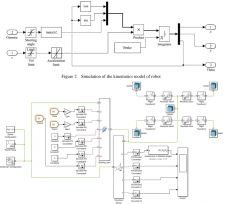
software has been addressed. Figure 2 shows the
implementation of Equations (3) to (5) in the Simulink
environment. Linear speed and steering angle as input,
and position and angle of the robot are considered as
output of this model.
In order to have a dynamic environment and visual
representation of the robot’s motion, the robot model is
interconnected individually in the SimMechanics of
Matlab software to allow the robot’s behavior in dealing
with various control algorithms observed by combining it
with Simulink environment. In Figure 3, a plan is visible
from this environment.
Figure 2 Simulation of the kinematics model of robot
In this simulation model, at first, different parts of the
robot, which are designed in SolidWorks software, are
brought to the SimMechanics environment by Solid
blocks. Blocks are assembled in this environment by
appropriate joints to show how well the robot behaves.
By placing a sensor on a robot, in order to report its
position and angles (such as the gyroscope sensor), these
robot features are available throughout the path. The
robot moves with constant velocity and the steering angle
is the only control variable.
The control commands to the simulated model have
been implemented from controllers written in the
Simulink. In addition, by reporting the amount of rotation
of each joint, in fact, will be an encoder on the each
wheel which produces output in radians per second. In
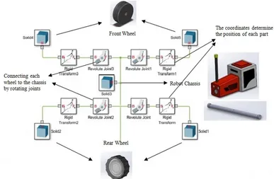
Figure 4, simulation of the robot and the transfer of
various parts of SolidWorks to the SimMechanics, along
with an explanation of each part, are presented.
Figure 4 Simulate a robot and transfer parts to the simulator SimMechanics
2.3 Control
This section firstly examined the robot movement
from an initial point to a target point (x*
, y*). A
proportional controller has been used to apply the input to
the kinematic model of the robot. To control the robot
speed, the following equation was used (Corke, 2011):
* 2 * 2
( ) ( )
V
v K= x −x + y −y (7)
Equation (7) calculates the velocity applied to the
model of robot by the controller. Also, the angle of the
robot at the target point and steering angle is also
obtained from the following equations.
*
* 1
*
tan y y
θ
x x
− −
=
− (8)
*
( )
s
γ=K θ −θ (9)
Also, tracking errors are obtained from reducing the
current position of the robot from the optimal input value
at any given moment and by the PID controller, these
errors are pushed to zero. Another important task for
robots is to move to a specific line and follow it. Consider the hypothetical ax+by+c=0 line. We need two controllers to control the steering. The first controller is designed to
control the steering in tracking the line, and the second
controller is designed to match the direction of the robot
with the hypothetical line (Corke, 2011):
2 2
( , , ) ( , ,1)a b c x y d
a b
⋅ =
+ αd =K dd Kd >0 (10)
* 1
tan a
θ
b
− −
= *
0( )
h h
α =K > θ −θ Kh>0 (11)
The above equations are the mathematical relations of
steering controllers for this maneuver. Finally, the steering
angle is obtained according to the equation as follow:
γ=Kdd+Kh(θ*–θ) (12)
Finally, the robot tracks the path that is generally
defined on the x-y plane. This path can be obtained by
should go through. The robot’s motion control in this case
is very similar to the one in which the robot moves to a
target point, With the difference that in this case the
target point changes (Corke, 2011):
The robot is always at a short distance (d*
) from the
target point. Therefore, the error is calculated as follow:
* 2 * 2 *
( ) ( )
e= x −x + y −y −d (13)
To control the speed at points where the error is zero,
we use a PID controller.
*
v i d
de
v K e K edt K
dt
= − +
∫
+ (14)To control the steering angle, as before, we use a
proportional controller.
*
* 1
*
tan y y
θ
x x
− −
=
− (15)
In Figure 5, tracking the path by the robot is
simulated from a primitive point in the plane. In this
block, Equations (18)-(21) are implemented in the
Simulink toolbox of MATLAB, and the robot follows it
after applying the optimal path. In Figure 6, the path of
the robot from the red center point is shown in order to
track the desired path.
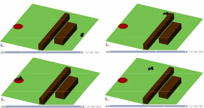
In Figure 7, the agricultural robot simulated in the
MATLAB mechanical simulator is tracking the path.
Figure 5 Simulate motion in a desired path
Figure 6 Simulated path of robot movement
2.4 Localization
Now, the robot positioning in the simulation
environment is performed using two methods, K.F. and
D.S. Also, the initial weighing to the sensors' results will
be explained and applied.
2.4.1 Dempster – Shafer’s Theory
Dempster-Shafer’s Theory of Evidence according to
many credible references, is the most powerful method in
data fusion. In fact, this method merges data at the
decision level. This method has the ability to integrate
any numerical, signal, and multi-dimensional data. One of
the areas that this tool and its features are underused is
the localization. In this paper, how D.S. Theory of
Evidence can be used in precise positioning of moving
objects was firstly shown, and then the performance of
this method in localization was compared with K.F.
method. D.S. theory is a generalization of the Bayesian
method that can handle sensor information defects. In the
event that all necessary information is available, all data
fusion methods provide a comprehensive and acceptable
approach. But in the face of lack of sensitivity and
sensitivity data, they are not reliable. Because in this case,
these methods should make assumptions about sensor
data which may not match on real data. Consequently,
conflicting results may be obtained. But D.S. theory is not
limited by model defects or previous information defects.
In this way, the evidence is determined solely on the basis
of the data obtained, and not with the assumed data. Thus,
this method is a quick and accurate tool for combining
incomplete data. For sensory data fusion using the D.S.
method, a given weight must be assigned to each data
source at any given time. For this purpose, firstly, by the
standard deviation of data, for the N last produced data,
the amount of data validation for each sensor is
determined. If the standard deviation of the N last data is
smaller than the specified value α, there are fewer jumps
and more confidence in that sensor, and if the standard
deviation is greater than that value, reliability will be less.
α and N values are empirically determined based on the
behavior of sensor data or expert opinion. Initially, the
variance of each sensor’s data is calculated:
2 2 1 1 ( ) N i i
σ x μ
N =
=
∑
− (16)2 1
2 2
Highly reliable level ( 1)
Poorly reliable level ( 2)
c σ α
c σ α
= ≤
= > (17)
With each new data, the variance of the N last data is
updated and the upper and lower levels of confidence are
specified. These levels are used in Shannon entropy
relations as follows: (Lu et al., 2016)
1 1 1 2 t c t t t c P c c = +
∫
∫
∫
, 2 2 1 2 t c t t t c P c c = +∫
∫
∫
(18)And the entropy criterion for each of the sensors is
obtained as follows (Lu et al, 2016):
2
2 1 log
c c
it c it it
H =
∑
= P P (19)Finally, by the entropy obtained for each sensor, and
using the formula below, its weight will be determined
(Lu et al, 2016):
2 2
1
1
( ) ( )
it I
it i it
W
H = H −
=
∑
(20)The greater the entropy of a sensor's data, the lower
the confidence level, and consequently the lower the
weight assigned.
2.4.2 Sensor Noise Simulation and Performance
Analysis of fusion Tools
Firstly, the positioning data of two sensor data
sources- Sensor 1: the GPS data and Sensor 2: the total of
inertial measurement unit (IMU) data and the rear wheel
encoders- is received from sensor blocks in the Simulink
toolbox, and re-simulated after adding noise and bias up
to 10% of the turmoil to those. Then, in the first step, for
a specific semicircular path, the sensor values are
combined by K.F. and D.S. separately. There are three
series of diagrams, each showing one of the robot
position parameters. In each series of charts, the output of
the simulated blocks of two sensor sources that are
coupled with noise, and the results of applying two data
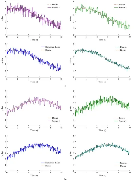
fusion tools are shown. In Figure 8(a), the parameter x, in
the Figure 8(b), the parameter y and in the Figure 8(c),
the parameter θ are analyzed in MATLAB simulation
toolbox. The performance of these two data fusion tools
is shown in a given time period and path. As indicated in
these diagrams, the red-dashed paths are the real robot
motions in the simulation environment, which is expected
to show by the ideal sensors. Purple and pale green colors
respectively for the first and second sensor sources. Also
the blue color shows the fusion of two noisy sensor data
by D.S. method and the dark green color shows the fusion
by the K.F. method. It is clear that the Kalman method
shows better performance in Gaussian noise.
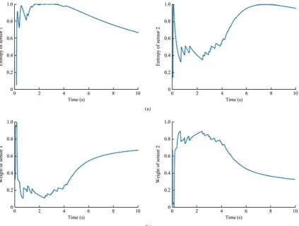
Figure 9(a) is the entropy graph of the two sensor
sources, and Figure 9(b) is the obtained weight graph
based on sensor data. As shown in these charts, the
entropy of the Sensor 1 is greater than the Sensor 2,
which indicates more disorder in GPS data than the
encoder plus IMU data and so, the reliability of the data is
less and the weight allocated to that sensor will be less.
(a)
(c)
Figure 8 Noise simulation diagrams and the results of applying the fusion tool to the robot position parameters
(a)
(b)
Figure 9 Entropy graph of sensor data and weight assigned to sensor sources
3 Results and discussions
As shown in Figure 8, K.F. seems to have a better
performance than D.S., but according to Figure 9, the
need to provide a benchmark for comparing the
performance of these two data fusion tools seems to be
necessary. For this reason, the mean absolute deviation
(MAD) and mean square error (MSE) criteria have been
used.
The MAD, also referred to as the ‘mean deviation’ or
sometimes ‘average absolute deviation’, is the mean of
the data’s absolute deviations around the data's mean: the
average (absolute) distance from the mean. ‘Average
general form with respect to a specified central point. The mean absolute deviation of a set {x1, x2, x3, …, xn} is
1 1 | ( ) | n i i
MAD x m x
n =
=
∑
− (21)Which n is the number of values and m(x) is the mean. MAD has been proposed to be used in place of standard
deviation since it corresponds better to real life. Because
the MAD is a simpler measure of variability than the
standard deviation. This method's forecast accuracy is
very closely related to the MSE method which is just the
average squared error of the forecasts. Although these
methods are very closely related, MAD is more
commonly used because it is both easier to compute
(avoiding the need for squaring) and easier to understand.
2 1 1 ˆ ( ) n i l i
MSE x x
n =
=
∑
− (22)Which ˆxl is predicted value.
The numbers in the table below belong to the x
variable in each simulation test and for each evaluation
criterion.
The simulation reported in the previous section has
been carried out six times for two different paths (a linear
path and a circular path). In the fifth and sixth tests, the
noise level applied to the Sensors is non-Gaussian noise.
Typical IMU/GPS integration approaches usually adopt
the Gaussian error assumption. However, in practice,
especially during off-road navigation and when several
sources of GPS interference are present, this assumption
does not hold. To this end, the best non-Gaussian noise
model is the Huber estimator using a robust estimator
algorithm, which is able to handle multipath GPS signals
as well as intentional and unintentional interferences.
Gaussian mixture models are based on the representation
of any non-Gaussian distribution as the sum of multiple
Gaussian densities with different weights (Karlgaard and
Schaubt, 2007).
For the IMU/GPS algorithm discussed here, the noise
is assumed to be composed of two Gaussian components.
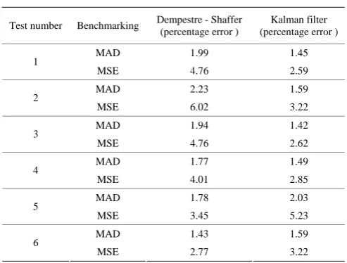
The results presented in Table 1 showed that the
performance of the D.S. method in sensor data fusion
associated with non-Gaussian noise was better than the
K.F. Since in real life the noise behavior was more
non-Gaussian, it seemed that the Dempster method would
perform better in dealing with real issues.
Table 1 Comparison of the performance of two data fusion tools
Test number Benchmarking Dempestre - Shaffer (percentage error )
Kalman filter (percentage error )
MAD 1.99 1.45
1
MSE 4.76 2.59
MAD 2.23 1.59
2
MSE 6.02 3.22
MAD 1.94 1.42
3
MSE 4.76 2.62
MAD 1.77 1.49
4
MSE 4.01 2.85
MAD 1.78 2.03
5
MSE 3.45 5.23
MAD 1.43 1.59
6
MSE 2.77 3.22
4 Conclusion
In this paper, tried to simulate controlling of an
agricultural tractor robot and it's localization in real
condition using Dempster-Shafer and Kalman filter
algorithms, as data fusion tools, in the MATLAB
software. In the control part of the robot, various control
scenarios were be carried out on the robot, including
tracking, moving toward the target point and moving to a
given line, and they are simulated in the mechanical
simulator of MATLAB (SimMechanics). In the field of
localization, the use of D.S. evidence theory as a tool for
data fusion and exploiting the strengths of this method
and comparing it with the K.F. for the best possible
implementation of collecting and processing sensory data
is one of the innovations of this paper. In this way, the
evidence is determined solely on the basis of real data.
This is a quick and accurate tool for incomplete data
fusion. Also, the initial weighting of sensors by entropy
method is one of the other innovations in this paper to
determine the confidence coefficient of each sensor and
to determine its weight. To apply the weight of each of
the sensors in this method as evidence theory, at the
decision level, entropy of sensor data is used. After the
implementation of data fusion methods and in order to
provide a scientific standard for comparing the above
methods, the simulation was repeated with the application
of Gaussian and non-Gaussian noise in different paths
and the localization information of these two methods in
these simulations was examined by two MAD and MSE
D.S. method when applying non-Gaussian noise which is
the reliability validation of the D.S. method in conditions
close to real conditions. The upcoming process is the
practical implementation of the localization and control
algorithms examined in this paper and use of the results
obtained from it.
References
Akhoundi, M. A. A., and E. Valavi. 2010. Multi-sensor fuzzy data fusion using sensors with different characteristics. arXiv
preprint arXiv: 1010.6096.
Betz, J. W., J. L. Prince, and M. G. Bello. 1989. Representation and transformation of uncertainty in an evidence theory framework. In Proc. of CVPR'89 IEEE Computer Society Conf.
on Computer Vision and Pattern Recognition, 646–652.San Diego, CA, USA, 4-8 June.
Bevly, D. M., R. Sheridan, and J. C. Gerdes. 2001. Integrating INS sensors with GPS velocity measurements for continuous estimation of vehicle sideslip and tire cornering stiffness. In
Proc. of the 2001 American Control Conf., 25–30. Arlington, VA, USA, 25-27 June.z
Boston, J. R. 2000. A signal detection system based on Dempster-Shafer theory and comparison to fuzzy detection.
IEEE Transactions on Systems, Man, and Cybernetics,Part C (Applications and Reviews), 30(1): 45–51.
Corke, P. 2011. Robotics, Vision and Control: Fundamental
Algorithms in MATLAB. 2nd ed. Springer International Publishing.
Denoeux, T., S. Li, and S. Sriboonchitta. 2018. Evaluating and comparing soft partitions: an approach based on Dempster-Shafer theory. IEEE Transactions on Fuzzy Systems, 26(3): 1231–1244.
Edan, Y. 1995. Design of an autonomous agricultural robot.
Applied Intelligence, 5(1): 41–50.
Fenton, N., B. Littlewood, M. Neil, L. Strigini, A. Sutcliffe, and D. Wright. 1998. Assessing dependability of safety critical systems using diverse evidence. IEE Proceedings-Software, 145(1): 35-39.
Ghahroudi, M. R., and A. Fasih. 2007. A hybrid method in driver and multisensor data fusion, using a fuzzy logic supervisor for vehicle intelligence. In 2007 International Conf. on Sensor
Technologies and Applications (SENSORCOMM 2007), 393-398. Valencia, Spain, November 2007.
Hall, D. L., and J. Llinas. 1997. An introduction to multisensor data fusion.Proceedings of the IEEE, 85(1): 6–23.
Karlgaard, C. D., and H. Schaubt. 2007. Huber-based divided difference filtering. AIAA Journal of Guidance, Control and
Dynamics, 30(3): 885–891.
Keicher, R., and H. Seufert. 2000. Automatic guidance for
agricultural vehicles in Europe.Computers and Electronics in
Agriculture, 25(1): 169–194.
Klein, L. A. 1993. Sensor and Data Fusion Concepts and Applications. Bellingham, WA, USA: Society of Photo-Optical Instrumentation Engineers (SPIE).
Li, W., Y. Huang, Y. Cui, S. Dong, and J. Wang. 2010. Trafficability analysis of lunar mare terrain by means of the discrete element method for wheeled rover locomotion.
Journal of Terramechanics, 47(3): 161–172.
Liu, Y., N. R. Pal, A. R. Marathe, and C. Lin. 2018. Weighted fuzzydempster-shafer framework for multi-modal information integration. IEEE Transactions on Fuzzy Systems, 26(1): 338–352.
Lu, C., K. Ying, and H. Chen. 2016. Real-time relief distribution in the aftermath of disasters–A rolling horizon approach.
Transportation Research Part E: Logistics and Transportation Review, 93: 1–20.
Mizushima, A., K. Ishii, N. Noguchi, Y. Matsuo, and R. Lu. 2011. Development of a low-cost attitude sensor for agricultural vehicles. Computers and Electronics in Agriculture, 76(2): 198–204.
Murakami, N., A. Ito, J. Dale Will, M. Steffen, K. Inoue, K. Kita, and S. Miyaura. 2006. Environment identification technique using hyper omni-vision and image map. In Proc. of the 3rd IFAC International Workshop Bio-Robotics, 317–320. Sapporo, Japan,
Murphy, R. R. 1998. Dempster-Shafer theory for sensor fusion in autonomous mobile robots. IEEE Transactions on Robotics
and Automation, 14(2): 197–206.
Nagasaka, Y., N. Umeda, Y. Kanetai, K. Taniwaki, and Y. Sasaki. 2004. Autonomous guidance for rice transplanting using global positioning and gyroscopes. Computers and Electronics
in Agriculture, 43(3): 22–-234.
Pagac, D., E. M. Nebot, and H. Durrant-Whyte. 1998. An evidential approach to map-building for autonomous vehicles.
IEEE Transactions on Robotics and Automation, 14(4): 623–629.
Park, J. J. 2016. Graceful navigation for mobile robots in dynamic and uncertain environments. Ph.D. diss., Mechanical Engineering Dept., University of Michigan.
Rakowsky, U. K. 2007. Fundamentals of the Dempster-Shafer theory and its applications to reliability modeling.
International Journal of Reliability, Quality and Safety Engineering, 14(06): 579–601.
Roberts, R. G., T. Graham, and T. Lippitt. 1998. On the inverse kinematics, statics, and fault tolerance of cable‐suspended robots.Journal of Robotic Systems, 15(10): 581–597.
Approximate Reasoning, 33(1): 1–49.
Shi, H., X. Li, W. Pan, K. S. Hwang, and Z. Li. 2017. A novel fuzzy three-dimensional grid navigation method for mobile robots. International Journal of Advanced Robotic Systems, 14(3): 1729881417710444.
Subramanian, V., T. F. Burks, and A. A. Arroyo. 2006. Development of machine vision and laser radar based autonomous vehicle guidance systems for citrus grove navigation. Computers and Electronics in Agriculture, 53(2):
130–143.
Subramanian, V., T. F. Burks, and W. E. Dixon. 2009. Sensor fusion using fuzzy logic enhanced kalman filter for autonomous vehicle guidance in citrus groves. Transactions of
the ASABE, 52(5): 1411–1422.