International Doctorate School in Information and Communication Technologies
DIT - University of Trento
A Tag Contract Framework for
Modeling Heterogeneous Systems
Thi Thieu Hoa Le
Advisor:
Professor Roberto Passerone
Universit`a degli Studi di Trento
In the distributed development of modern IT systems, contracts play a vital
role in ensuring interoperability of components and adherence to
specifica-tions. The design of embedded systems, however, is made more complex
by the heterogeneous nature of components, which are often described using
different models and interaction mechanisms. Composing such components
is generally not well-defined, making design and verification difficult.
Sev-eral denotational frameworks have been proposed to handle heterogeneity
using a variety of approaches. However, the application of heterogeneous
modeling frameworks to contract-based design has not yet been investigated.
In this work, we develop an operational model with precise heterogeneous
denotational semantics, based on tag machines, that can represent
hetero-geneous composition, and provide conditions under which composition can
be captured soundly and completely. The operational framework is
imple-mented in a prototype tool which we use for experimental evaluation. We
then construct a full contract model and introduce heterogeneous
compo-sition, refinement, dominance, and compatibility between contracts,
alto-gether enabling a formalized and rigorous design process for heterogeneous
systems. Besides, we also develop a generic algebraic method to
synthe-size or refine a set of contracts so that their composition satisfies a given
Keywords
This dissertation would not have been completed without the support of
many individuals and institutions.
I would like to express my utmost gratitude to my advisor, Professor Roberto
Passerone, for his guidance and support through years of my study. His
expertise, advice and time have proven to be indispensable in my academic
and life journey, especially in moments when I feel lost of my research
track. His encouragement has also been a great motivation for me to go on
with this research work.
I have had several great supporters at the research institution INRIA/IRISA
in Rennes, France ever since I did my internship there. Professor Axel
Legay and Doctor Uli Fahrenberg were my supervisors while I was an
in-tern at INRIA. This research work was partially inspired by them and I
owe them a special thanks for their elaborated discussion and fruitful
col-laboration which is spread throughout this thesis work.
The faculty and staff at University of Trento have all provided me with
much help and support for which I am thankful. I would also like to thank
all the members of the EECS lab with whom I have shared research ideas
as well as difficulties in research life.
Finally, I owe the greatest thanks to my caring and patient husband whose
unconditional love and support has always kept me on task and been my
1 Introduction 1
1.1 The Context . . . 1
1.2 Thesis Contributions . . . 3
1.2.1 A Sound Underlying Representation . . . 3
1.2.2 Heterogeneous Contract-based Design Methodology 4 1.3 Structure of the Thesis . . . 5
2 State of the Art 7 2.1 Theory of Heterogeneous Composition . . . 7
2.2 Theory of Interface and Contract . . . 9
3 Modeling and Verification of a Distributed HCS 15 3.1 HCS Description . . . 15
3.2 Parametric Modelling . . . 17
3.2.1 Packet Release Modeling . . . 17
3.2.2 Schedulability Checker Modeling . . . 18
3.3 Parametric Analysis . . . 21
4 Tag Systems 25 4.1 Homogeneous Composition . . . 26
5 Tag Machines 31
5.1 Composition of Tag Machines . . . 34
5.1.1 Homogeneous Composition . . . 34
5.1.2 Heterogeneous Composition . . . 35
5.2 Interoperable TMs and Composition Soundness . . . 38
5.3 Self-synchronizing TMs and Composition Completeness . . 48
5.4 An Automotive Case Study . . . 51
5.4.1 Description . . . 51
5.4.2 Tag Machine Script Language . . . 54
5.4.3 Tag Machine Simulator . . . 55
5.4.4 Evaluation . . . 56
6 Tag Contracts 59 6.1 Tag Machine Operators . . . 59
6.1.1 Tag Machine Refinement . . . 59
6.1.2 Tag Machine Quotient . . . 61
6.1.3 Tag Machine Conjunction . . . 63
6.2 Tag Contracts . . . 64
6.2.1 Tag Contract Refinement . . . 69
6.2.2 Tag Contract Dominance . . . 71
6.2.3 Tag Contract Composition . . . 72
6.2.4 Tag Contract Compatibility . . . 74
7 Contract Synthesis 77 7.1 Homogeneous Contract Synthesis . . . 78
7.1.1 Contract Composition . . . 79
7.1.2 Contract Decomposition . . . 83
7.1.3 Contract Synthesis . . . 84
7.1.4 Trace-based Contract Synthesis . . . 87
8 Conclusion 109
3.1 Fixed parameter settings . . . 22
7.1 Rules for combing modal specification using modal operators
3.1 Heterogeneous Communication System . . . 16
3.2 Packet streams in HCS . . . 16
3.3 PTP and audio task activation automata . . . 18
3.4 Schedulability checker for PTP packets . . . 19
3.5 Schedulability checker for audio packets . . . 20
3.6 Audio (in)feasibility regions for ∆ = 0,3,5,7 and PTP (in)feasibility regions in two experiments . . . 23
5.1 Non-interoperable TMs . . . 39
5.2 Interoperable TMs . . . 43
5.3 A simple water tank system . . . 45
5.4 Interoperable TMs accepting Σ1 . . . 49
5.5 An automotive engine control model . . . 52
5.6 High-level description of a piston TM and its morphism . . 54
5.7 Basic schema of TM simulator . . . 55
5.8 Basic schema of TM simulator . . . 56
5.9 The evolutions of x(t) and a(t) without and with control . 57 6.1 The tank contract . . . 65
6.2 The controller contract . . . 65
6.3 Mu . . . 76
7.1 Commutative diagram for and f . . . 85
7.3 A modal contract . . . 92
7.4 Modal contracts for a simple message system . . . 95
7.5 Synthesis based on heterogeneneous quotient and projection 97 7.6 The tank contract . . . 105
7.7 The controller contract . . . 106
7.8 The desirable water control behavior . . . 107
Introduction
1.1
The Context
Modern computing systems are increasingly being built by composing
com-ponents which can be developed concurrently by different design teams. In
such a development paradigm, the distinction between what is constrained
on environments, and what must be guaranteed by a system given the
constraint satisfaction, reflects the different roles and responsibilities in
the system design procedure. Such distinction can be captured by a
com-ponent model called contract [42]. Formally, a contract (C) is a pair of
assumptions (A) and guarantees (G) (i.e. C = (A,G)) which intuitively are properties that must be satisfied by all inputs and outputs of a design,
respectively. The separation between assumptions and guarantees supports
the distributed development of complex systems and allows subsystems to
synchronize by relying on associated contracts.
In the particular context of embedded systems,heterogeneity is a typical
characteristic since these systems are usually composed from parts
devel-oped using different methods, time models and interaction mechanisms.
Such heterogeneity usually appears across different layers of abstraction
in the design flow, making the evaluation of whether certain properties
1.1. THE CONTEXT
level become extremely difficult. It has been often the case that
hetero-geneous compositional mechanism is not sufficiently well-defined to enable
the verification of some system property from the known properties of its
components. To deal with heterogeneity, several modeling frameworks have
been proposed oriented towards the representation and simulation of
het-erogeneous systems, such as the Ptolemy framework [39], or towards the
unification of their interaction paradigms, such as those based on tagged
events [37]. The former is geared towards the representation and simulation
of heterogeneous systems while the latter can capture different notions of
time and interaction paradigms, including physical time, logical time
(syn-chronous and asyn(syn-chronous), precedence relations, etc., and relate them
by mapping tagged events over a common tag structure [5].
Due to the significant inherent complexity of heterogeneity, there have
been only very few attempts at addressing heterogeneity in the context of
contract-based models. For instance, the HRC model from the SPEEDS
project1 was designed to deal with different viewpoints (functional, time,
safety, etc.) of a single component [7, 19]. However, the notion of
hetero-geneity in general is much broader than that between multiple viewpoints,
and must take into account diverse interaction paradigms. Meanwhile,
het-erogeneous modeling frameworks have not been related to contract-based
design flows. This has motivated us to study a methodology which allows
heterogeneous systems to be modeled and interconnected in a
contract-based fashion.
The central issues when studying such a methodology includes
refine-ment, composition and compatibility between contracts in order to enable
a formalized and rigorous design process for heterogeneous systems.
Be-sides, it is often desirable to study how to fix individual contracts so as to
make their composition satisfies or refines an abstract specification
sented as another contract. This is an instance of the well-known classical
synthesis problems:
“Can we construct a model that satisfies some given specification?”.
This problem is very popular when designing systems in a top-down
de-composing fashion because the overall contract’s decomposition into
sub-contracts is not always satisfactory.
1.2
Thesis Contributions
Our long term objective is to develop a modeling and analysis framework
for the specification and verification of both heterogeneous components
and contracts.
1.2.1 A Sound Underlying Representation
As a start, we have modeled a simplified version of a distributed
Heteroge-neous Communication System (HCS) such as one that one that could be
found on board of air-crafts [27], using timed automata [1] augmented with
parameters. Different components of a HCS system including server,
com-munication network and devices are modelled as timed automata which
al-lows us to compose them together and reason on their composite behavior.
Since no heterogeneous machinery for composing different components has
been available as will be discussed in Section 2.1, assembling the
compo-nents of HCS is done homogeneously. The case study has provided us with
a valuable understanding regarding how time can be captured in different
models of time such as Uppaal [31], NuSMV [16], HyDI [17] and regarding
the complexity of modeling various components through a homogeneous
1.2. THESIS CONTRIBUTIONS
With this understanding, the framework that we aim at developing
should be able to support formal correctness proofs as obtained in the
HCS case study. To this end it must employ an underlying (or
interme-diate) semantically sound model that can be used to represent different
computation and interaction paradigms uniformly. Because simulation is
an essential design activity, the model must also be executable. At the same
time, the semantic model must be able to retain the individual features of
each paradigm to avoid losing their specific properties. In particular, the
framework must interact with the user through a front end that exposes
familiar models that feel native and natural. In this work, we focus on
the intermediate semantic model and defer the discussion on how specific
front ends may be constructed to our future work. For this purpose, we
advocate the use of Tag Machines (TMs) as a suitable semantic model
for system specification. We have chosen to use this formalism for our
work, as it provides an operational representation based on rigorous and
proven semantics. Tag Machines can be used to represent homogeneous
systems [6] and to achieve our goal, we extend TMs to encompass the
heterogeneous context. In particular, we study the relation between
com-position of TMs with that of their denotational semantics. We first review
and correct certain aspects of TMs, and provide conditions under which the
operational model can fully and compositionally capture the denotational
representation. We have also developed a simulation engine that supports
heterogeneous TMs, with which we experimentally evaluate our results on
a significant case study.
1.2.2 Heterogeneous Contract-based Design Methodology
Our second objective is to develop a methodology for modeling
heteroge-neous systems in a contract-based fashion. In this goal, we build a contract
relations between contracts such as satisfaction, refinement, composition
and compatibility.
To achieve such goal, we rely on a generic meta-framework [4] that
we extend with tags and mappings between tags to define model
inter-actions. In particular, we study the contract synthesis capability in the
homogeneous and heterogeneous contexts. For homogeneous contracts, we
propose decomposing conditions for a set of contracts {C1, . . . ,Cn} under
which the contract decomposition can be verified, and thereby proposing
a generic synthesis strategy for fixing wrong decompositions. For
heteroge-neous contracts, we limit the size of contract set to two in order to make
the synthesis procedure manageable and simple.
1.3
Structure of the Thesis
The rest of the thesis is organized as follows.
• In Chapter 2, we review the state of the art with respect to the evolu-tion of theories of heterogeneous composievolu-tion as well as that of theories
of interface and contract.
• In Chapter 3, we present a summary of our preliminary investigation on modeling a distributed heterogeneous systems.
• In Chapter 4, we recall notions of tags, behaviors, denotational tag systems and their composition.
• In Chapter 5, we first describe how TMs are extended to represent heterogeneous systems and then discuss soundness and completeness
of the TM composition. We also demonstrate the application of our
1.3. STRUCTURE OF THE THESIS
• In Chapter 6, we present our tag contract framework for modeling heterogeneous systems built on top of TM operations such as
com-position, quotient, conjunction and refinement. Also in this chapter,
we discuss an application of our methodology to a simplified water
control problem and model it using incrementing TMs. The material
of Chapter 5 and Chapter 6 is mostly taken from [36, 35].
• In Chapter 7, we show how to synthesize a contract set in order to make their composition refine an overall contract when necessary in
both homogeneous and heterogeneous contexts.
State of the Art
2.1
Theory of Heterogeneous Composition
Heterogeneity theory has been evolving actively to assist designers in
deal-ing with heterogeneous composition of components with various Models of
Computation and Communication (MoCC). The idea behind these
theo-ries and frameworks is to be able to combine well-established specification
formalisms to enable analysis and simulation across heterogeneous
bound-aries. This is usually accomplished by providing some sort of common
mechanism in the form of an underlying rich semantic model or
coordina-tion protocol. In this work we are mostly concerned with these lower level
aspects.
One such approach is the pioneering framework of Ptolemy II [39], where
models, calleddomains, are combined hierarchically: each level of the
hier-archy is homogeneous, while different interaction mechanisms are specified
at different levels in the hierarchy. In the underlying model, intended for
simulation, each domain is composed of a scheduler (the director) which
exposes the same abstract interface to a global scheduler which coordinates
the execution. This approach, which has clear advantages for simulation,
has two limitations in our context. First, it does not provide access to the
2.1. THEORY OF HETEROGENEOUS COMPOSITION
to establish relations to only the models of computation, and not to the
heterogeneous contracts of the components. Secondly, the heterogeneous
interaction occurs implicitly as a consequence of the coordination
mecha-nism, and can not be controlled by the user. The metroII framework [20]
relaxes this limitation, and allows designers to build model adapters
di-rectly. However, metroII treats components mostly as black boxes using
a wrapping mechanism to guarantee flexibility in the system integration,
making the development of an underlying theory complex. These and
other similar frameworks are mainly focused on handling heterogeneity at
the level of simulation.
Another body of work is instead oriented towards the formal
represen-tation, verification and analysis of these system. The BIP framework uses
the notion of connector, on top of a state based model, to implement both
synchronous and asynchronous interaction patterns [9]. Their relationship,
however, can not be easily altered, and the framework lacks a native
no-tion of time. Benveniste et al. [5] propose a heterogeneous denotano-tional
semantics inspired by the Lee and Sangiovanni-Vincentelli (LSV)
formal-ism of tag signal models [37], which has been long advocated as a unified
modeling framework capable of capturing heterogeneous MoCC. Starting
from the LSV model, the authors have derived their preferred variation of
tag system model where a system is modeled as a set of behaviors. Each
behavior is modeled as a set of signals which are sequences of events and
each event is characterized by a data value and a tag. In both models, tags
play an important role in capturing various notions of time, where each tag
system has its own tag structure expressing an MoCC and homogeneous
systems share the same tag structure while heterogeneous systems have
different tag structures. Composing such systems is thus done by applying
mappings between different tag structures.
of homogeneous tag systems. They are quite expressive, and ways to map
traditional interaction paradigms have been reported in the literature [6].
They have also been applied to model a job-shop specification [23] such
that the composite tag machine represents the overall job-shop specification
and any trace of the machine from the start to the final state results in
a valid job-shop schedule. For the purpose of studying the asymptotic
throughput of an infinite job-shop schedule, the authors have proposed a
new tag structure to capture the aspect of performance evaluation and an
algorithm for evaluating the throughput of job-shop schedules based on
tag machine. The algorithm has also been applied to an SDFG model of
periodic self-timed executions and a heterogeneous system composed of a
dataflow component and a discrete-event component.
Alternatively, tag systems can be represented by functional actors
form-ing a Kleene algebra [24]. The approach is similar to that of Ptolemy II in
that both use actors to represent basic components.
2.2
Theory of Interface and Contract
The notion of contract was first introduced by Bertrand Meyer in his
design-by-contract method [42], based on ideas by Dijkstra [25],
Lam-port [30], and others, where systems are viewed as abstract boxes
achiev-ing their common goal by verifyachiev-ing specified contracts. Such a technique
essentially guarantees that methods of a class provide some post-
condi-tions at their termination, as long as the pre-condicondi-tions under which they
operate are satisfied. The class itself can have invariants that must be
true at all states of the class and in order to offer safe substitutability, a
subclass is only allowed to weaken the pre-conditions and strengthen the
post-conditions. Design-by-contract has then been adopted in
2.2. THEORY OF INTERFACE AND CONTRACT
activities are specified for a designer to follow in order to obtain complete
component specifications which include the component interface, the
inter-component collaboration and a set of contracts in forms of pre-conditions,
post-conditions and invariants that apply to the component. The
imple-mentation patterns for pre-conditions, post-conditions and invariants were
subsequently formalized to automatically generate component skeletons
that already implemented such constraints [18].
To allow effective reuse of components in component-based design flows,
De Alfaro and Henzinger introduced a light-weight formalism based on
automata to document the component specification, called interface
au-tomata [21]. This formalism establishes a more general notion of contract
where pre-conditions and post-conditions, which originally appeared in the
form of predicates, are generalized to behavioral interfaces so as to capture
the temporal Input/Output (I/O) behaviours of a component. The I/O
actions are expressed by transitions labelled with a “?”/”!”
correspond-ingly. Although being syntactically similar to I/O automata proposed by
Lynch [40], interface automata are not necessarily input-enabled and at
each of its states, some inputs may not be accepted. By this, interface
automata express the assumption that the environment may never
gener-ates those inputs and thus input actions are under the environment
con-trol. Meanwhile, all outputs are controlled by the component itself, hence
are under the component responsibility. Although the assumptions and
guarantees are not handled explicitly, interface automata do capture the
different roles and responsibilities of a component and its environment.
The central issues when introducing the formalism of interface automata
are compatibility, composition and refinement. The authors highlight the
issue of checking compatible interfaces from two views: pessimistic versus
optimistic, and advocate the latter view in which two component interfaces
optimistic view, the composition of two interface automata is obtained by
restricting the product automaton to the set of compatible states from
which there is some environment that can prevent going to error states.
Then based on alternating simulation [2], the authors formalize the
rela-tion between an interface specificarela-tion and its implementarela-tion by means
of refinement, stating that an interface refines another if it has weaker
in-put assumptions and stronger outin-put guarantees. This definition allows a
component P to always be replaced with a more refined version Q pro-vided that they are connected to the environment by the same inputs. An
important connection between refinement and compatibility, which
cap-tures also the essence of component-based design, is also exposed through
this definition. That is the designer of the environment needs to ensure
only compatibility with the component specificationP which subsequently guarantees compatibility with the component implementation Q.
The alternating refinement, in fact, has a drawback when it fails to
enforce that the implementation does any useful activities at all. Larsen
et.al.’s subsequent introduction of modality into the interface theory [32]
helps to rule out such a trivial implementation since as long as some
tran-sition in the specification automata is associated with a must modality, it
must appear in any implementation. In the modal context, modal
refine-ment requires that the specification can mimic all allowed steps (marked
with a may modality 3) made by an implementation and an implemen-tation needs to match all required steps (marked with a must modality 2) made by the specification. The authors then show that the alternating refinement actually coincides with the modal refinement if all output
tran-sitions are assigned with 3, inputs with 2 and the may transition relation is made input-enabled. They further define the composition operator for
modal interface similarly to that of interface automata. However, Raclet
2.2. THEORY OF INTERFACE AND CONTRACT
it is not monotonic with respect to modal refinement as claimed, thereby
failing to ensure that two compatible interfaces may be implemented
sep-arately (call independent implementability in [32]). A correction has also
been proposed by the authors, resulting in the notion of relaxed
composi-tion. Such notion relaxes all constraints on the future of the runs that drive
the composition to a state where one interface may produce an output that
may not be accepted as input by the other. The relaxed composition refers
to such state as a “universal” state, meaning every action is assigned with
a may modality.
Another core contribution made by Raclet et.al. [45] is the unification
of two theories: interface automata [21] and modal specification [33] into
a new theory addressing also the problem of dissimilar alphabets which
was missing in previous work. It is worth noting that Larsen el.al.’s modal
interfaces [32] can be viewed as a modal specification except for the modal
composition operator and the occurrence of Input/Output distinction.
The contract theory has been evolving in parallel with the interface
theory. Researchers from the SPEEDS project have attempted to use a
set of constraints (i.e. pairs of Assumption/Guarantee), to describe the
expected behaviour of a component (i.e. a set of traces or runs) [7]. The
differentiation between assumptions and guarantees, which is implicit in
in-terface automata or modal specification, is made explicit in the trace-based
contract framework of the SPEEDS HRC model [7, 8]. Relevant notions
such as composability, compatibility and dominance are formalized for
con-tracts. Composability is a purely syntactic criterion on component profiles
which consists of uncontrolled and controlled ports, and compatibility is
defined as the receptiveness of the composite assumption with respect to
the composite ports under the component’s control. That is for any
se-quence of values on the controlled ports, there exists some environment
dominance to distinguish it from the refinement between implementations
of the contracts, following the usual scheme of weakening the assumptions
and strengthening the guarantees.
The relationship between specifications of component behaviors and
contracts is further studied by Bauer et al. [4] where a contract framework
can be built on top of any specification theory equipped with a composition
operator and a refinement relation which satisfy certain properties. The
mentioned trace-based contract theories [7, 8] are also demonstrated to be
instances of such framework. We take advantage of this formalization in
this work to construct our tag contract theory. In addition, this
formal-ization enables verifying if a contract can be decomposed into two other
contracts by checking if that contract can dominate the others. Therefore
we make a further advantage of such dominating notion and generalize it
to a set of n homogeneous contracts and construct generic decomposing
conditions for the homogeneous contract set.
The verification problem of decomposing a contract into a set of
con-tracts was also studied by Cimatti et al. [15] and was addressed by
property-based proof systems with SMT-property-based model checking techniques. The
contract specifications allowed in such systems, however, are trace-based
only. Our decomposing conditions can instead deal with generic contract
specifications including both trace-based and modal ones.
Assume-guarantee reasoning has also been applied extensively in
declar-ative compositional reasoning [22] to help prove properties by decomposing
the process into simpler and more manageable steps. Our objective is
con-ceptually different: assumptions specify a set of legal environments and are
used to prove (or disprove) contract compatibility and satisfaction. In
con-trast, classical assume-guarantee reasoning uses assumptions as hypotheses
to establish whether a generic property holds. Naturally, this technique
trans-2.2. THEORY OF INTERFACE AND CONTRACT
formation and formalization. In case of unsuccessful termination, AGR
can also provide a counterexample showing how the property can be
vio-lated. Such a counterexample can then be used to synthesize the model
so as to satisfy a given property [38]. However, this synthesis strategy is
only applicable for systems with trace-based semantics. Viewing the same
assume-guarantee synthesis problem as a game, Chatterjee et al. solve it
by finding a winning strategy on the global system state graph, but the
method does not guarantee the inclusion of all traces satisfying the
spec-ification [12]. The synthesized model was shown to be a subset of that
synthesized by counterexample-based synthesis [38]. Unlike these concrete
notions of synthesis, ours is more generic since it is not tied to the system
semantics. Moreover, while the application of our synthesis strategy to
generic contract-based systems is direct and straightforward, the
general-ization of the previous approaches has not been studied and would require
Modeling and Verification of a
Distributed HCS
In this section, we present a summary of our preliminary work on modelling
a distributed real-time system and refer to our technical paper [34] for the
comprehensive reading.
3.1
HCS Description
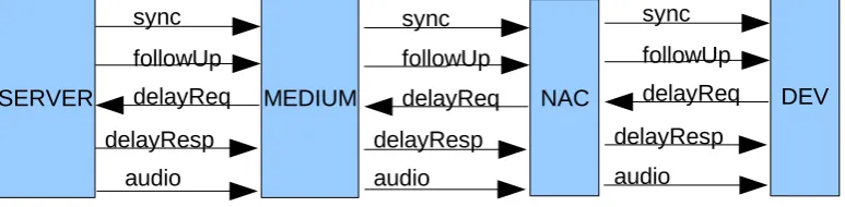
We have taken as a case study a simplified version of an HCS system which
consists of a common server and many devices communicating through
Network Access Controllers (NACs) as shown in Figure 3.1.
In the case study, we focus on audio devices which are required to
dis-tribute music and audio announcements to the main cabin. In addition,
the devices must reproduce the audio at synchronized instants, hence the
importance of the server-device clock synchronisation and their
implemen-tation of the Precision Time Protocol (PTP) [44]. The audio stream is
transmitted through the network. Each audio packet is sent by the server
everyaudP eriod (timeunits or tus) and characterized by the time it has to
be played at the device tplay. The transmission priority of PTP messages
3.1. HCS DESCRIPTION
Figure 3.1: Heterogeneous Communication System
transmission of an audio packet will not be preempted by a PTP message.
The packet streams can be shown logically as in Figure 3.2.
Figure 3.2: Packet streams in HCS
An PTP (Audio) packet transmitted through the network medium
in-curs a transmission delay C1(C2). These two quantities can be considered
as design parameters and are related to the packet size and to the channel
bitrate.
The model of HCS resembles a contract-based model. As long as the
assumption is respected (i.e. the parameter setting of C1 and C2 lies
streaming and clock synchronization (i.e. that the system will not
en-counter any Error state) can be guaranteed. In this case study, we are
interested in computing and representing the assumption on HCS
environ-ment, or in other words, verifying whether there are parameter settings
that allow the composite automaton to stay away from an Error state. To
do so, we employ parametric timed automata which are an extension of
the classical timed automata [1] and adapt the methodology for
paramet-ric analysis of real-time systems proposed in [14] to derive regions of free
design parameters that can provide such guarantee.
3.2
Parametric Modelling
Even the simplified HCS is too complex to be parametrically modelled
completely. Therefore, we have worked out an abstraction of the system to
limit the state space and to concentrate in isolation on each outstanding
issue (the non-preemptive scheduler, the different criticality of the timing
constraints, etc.).
The abstract model consists of two parts. The first models the release
of the packets on the network according to a periodic pattern. The second
models the network and device, including the scheduling policy and the
real-time constraints which can be hard or firm real-time constraints.
3.2.1 Packet Release Modeling
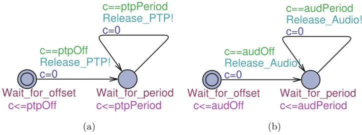
We model the release of packets as activation automata, shown in
Fig-ure 3.3. Each stream of packets is characterized by the offset for the first
release (transition from initial state to the second state), and is then
pe-riodic afterwards (self transition on the second state). A release signal is
emitted every time a transition is taken, and is used to synchronize the
3.2. PARAMETRIC MODELLING
c<=ptpPeriod c<=ptpOff
Release_PTP!
Release_PTP!
Wait_for_period Wait_for_offset
c=0
c=0
c==ptpPeriod
c==ptpOff
(a)
c<=audPeriod c<=audOff
Release_Audio!
Release_Audio!
Wait_for_period Wait_for_offset
c=0
c=0
c==audPeriod
c==audOff
(b)
Figure 3.3: PTP and audio task activation automata
3.2.2 Schedulability Checker Modeling
The remaining part of the system is modelled as a set of schedulability
checkers [14] that are non-preemptive, i.e. a transmission will not be
in-terrupted if it has already started. The schedulers are also prioritized, so
that when there is no ongoing transmission and many packets are ready,
the PTP packets go first and the audio packets back off.
The scheduler checker for PTP packets is shown in Figure 3.4, where:
• D1 is the deadline of PTP packets,
• C1/C2 are the transmission time of PTP/audio packets
• task denotes the currently-executed task,
• n1 andn2 record the number of PTP and audio packets released during
the current execution
• c is a clock accumulating the time since the task queues were last idle
• r is the sum of the time needed to complete all tasks released since the checker was last idle.
The model of the Audio checker is similar to but simpler than the PTP
Error
Busy
Check Idle
Release_Audio?
c==0 && task==2
Release_PTP?
r=r+C1+C1*n1-C2
c==r && n1==0 && n2>0
r=C2, task=2, c=0, n2=n2-1
c==r && n1>0
r=C1, task=1, c=0, n1=n1-1
c==0 & task==2
Release_PTP?
task=1, r=C1, n2=n2+1
c<r && c==D1
Release_PTP?
(c<r) && (c>0 || task==1)
Release_PTP? r=r+C1+C1*n1-c, c=0 c<r Release_Audio? n2=n2+1
(c<r) && (c>0 || task==1)
Release_PTP? n1=n1+1 c==r && n1==0 && n2==0 Release_PTP? task=1, c=0, r=C1, n1=0, n2=0 Release_Audio? task=2, c=0, r=C2, n1=0, n2=0
c==r && c<=D1
Release_PTP?
c=0, r=C1
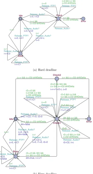
Figure 3.4: Schedulability checker for PTP packets
of audio packets and driftDelta is introduced to account for the offset
time of the local clock compared to the server clock. The worst case
hap-pens when the local clock is substantially slower than the server clock and
thus when an audio packet is received, the actual deadline to be verified
would be D2 −driftDelta instead of D2.
In fact, the requirement of no deadline miss (hard deadline) is difficult to
obtain in real-time environments. Therefore, in order to make the analysis
more practical, the requirement is relaxed by allowing an audio packet to
sometimes miss its deadline (firm real-time constraint). A firm real-time
constraint is given by a deadline and by a couple (m, n) meaning that m
deadlines can be missed every n jobs [41]. In our case study, a packet may
3.2. PARAMETRIC MODELLING Error Busy Check Idle Release_Audio? c<r && c==D2-driftDelta c>0 && c<r && c<D2-driftDelta Release_PTP? c==0 Release_PTP? r=r+C1 c<r Release_Audio? r=r+C2-c, c=0 c<r Release_Audio? r=r+C2 c<r Release_PTP? r=r+C1 c==r Release_PTP? c=0, r=C1 Release_Audio? c=0, r=C2 c==r && c<=D2-driftDelta Release_Audio? c=0, r=C2
(a) Hard deadline
Check2
Error
Busy
Check1 Idle
c==r && c<=D2-driftDelta c<r && c==D2-driftDelta
r2>0 && !dm && c<r && c==D2-driftDelta
r=r+r1+r2-c, c=0
r2>0
Release_Audio?
r2>0 && c>t && c<r && c<D2-driftDelta
Release_PTP?
r2>0 && c==t
Release_PTP?
r1=r1+C1
r2==0 && !dm && c<r && c==D2-driftDelta
dm=true, r=r+r1
r2==0 && c<r && c<D2-driftDelta
Release_Audio?
r2=C2, t=c
dm && c<r && c==D2-driftDelta r2==0 &&
c>0 && c<r && c<D2-driftDelta Release_PTP? r1=r1+C1 c==0 Release_PTP? r=r+C1 c<r Release_Audio? r=r+C2-c, c=0, r1=0, r2=0
c<r Release_Audio? r=r+C2, dm=false c<r Release_PTP? r=r+C1 c==r Release_PTP? c=0, r=C1 Release_Audio? c=0, r=C2, dm=false
c==r && c<=D2-driftDelta
dm=false
Release_Audio?
c=0, r=C2, r1=0, r2=0
(b) Firm deadline
deadline (m = 1, n = 2). The checkers for both constraints are shown in
Figure 3.5.
We introduce four new variables: dm is a boolean variable used to
cap-ture the fact that one deadline miss has already happened (dm = true),
r1 is a real variable used to record the total execution time of all PTP
in-stances released after the currently-checked instance and before a deadline
miss or the next audio arrival, r2 marks the next audio arrival whose time
is marked in t.
Intuitively, the transitions can be interpreted as follows:
• The transitions to Idle are taken when the task instance being checked in Check or a sequence of tasks arrived in Busy, has finished execution.
• The transitions to Busy are taken when an instance of task PTP or Audio is released. Self-loops are taken to queue the newly-released
instances and to retrieve them when the current execution has finished.
• The transitions to Check are taken when a PTP instance is (non-deterministically) chosen for checking. Before verifying the deadline,
the execution (or transmission) time of all other PTP instances in the
queue must be taken into account as they would be scheduled before
the current instance.
• The transition to Error is taken when the currently-executed instance misses its deadline.
3.3
Parametric Analysis
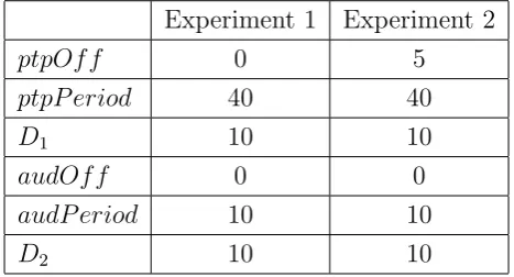
We have performed several experiments with a diverse set of parameters
and the results of two such experiments which differ in the amount of offset
3.3. PARAMETRIC ANALYSIS
Experiment 1 Experiment 2
ptpOf f 0 5
ptpP eriod 40 40
D1 10 10
audOf f 0 0
audP eriod 10 10
D2 10 10
Table 3.1: Fixed parameter settings
section. For the checker shown in the previous section, the free parameters
are the transmission times C1 and C2. The values of the fixed parameters
for each of the experiments are shown in Table 3.1.
Modelling the time aspect of HCS is possible in both Uppaal [31] and
NuSMV [16]. However, capturing a specific instant of time cannot be done
in Uppaal as so far it has supported only integer variables. Another
impor-tant limitation of the Uppaal model is that it only answers yes/no to the
verification problem without providing further feedback for the designers
regarding how to adjust parameters so that the system remains feasible.
To do parametric analyses on HCS, we have modelled it using NuSMV
and by adapting the parametric modelling tool [14] built upon NuSMT
[11], we have derived the feasibility (not shaded) and infeasibility (shaded)
regions for the PTP checker shown in Figure 3.6. The regions for the Audio
checker under a hard and firm real-time requirement are also shown in the
same figure where driftDelta(denoted as ∆) is introduced to account for
the offset time of the local clock compared to the server clock. By joining
the PTP and Audio feasibility regions together, we can obtain the regions
0 2 4 6 8 10
0 2 4 6 8 10
C2 C1 ∆=0 ∆=3 ∆=5 ∆=7
(a) Task audio, hard deadline, exp.1
0 2 4 6 8 10
0 2 4 6 8 10
C2 C1 ∆=0 ∆=3 ∆=5 ∆=7
(b) Task audio, hard deadline, exp.2
0 2 4 6 8 10
0 2 4 6 8 10
C2 C1 ∆=0 ∆=3 ∆=5 ∆=7
(c) Task audio, firm deadline, exp.1
0 2 4 6 8 10
0 2 4 6 8 10
C2 C1 ∆=0 ∆=3 ∆=5 ∆=7
(d) Task audio, firm deadline, exp.2
0 2 4 6 8 10
0 2 4 6 8 10
C2
C1
(e) Task PTP, exp.1
0 2 4 6 8 10
0 2 4 6 8 10
C2
C1
(f) Task PTP, exp.2
Tag Systems
We use denotational tag systems as our semantic domain [5, 37]. In
intu-itive terms, a tag system is a representation of the behaviors of a
compo-nent in terms of sets of events that take place at its interface, intended as a
collection of visible ports. Tags, which are associated to every event,
char-acterize the temporal evolution of the behaviors. By changing the structure
of tags, one can choose among different notions of time. Formally, a tag
structure T is a pair (T,≤) where T is a set of tags and ≤ is a partial order on the tags. To distinguish the tag order of T, we refer to it as ≤T when necessary. The ordering among tags is used to resolve the ordering
among events at the system interface. For instance, by using the set of real
numbers as tags, with their usual ordering, one can place events anywhere
in real time. Conversely, a set of partially ordered symbolic tags can be
used to express precedence between events in a branching-time setting.
Events occur at the interface of a component. A component exposes a
set V of variables (or ports) which can take values from a set D. An event
is a snapshot of a variable state, capturing the variable value at some point
in time. Formally, an event e on a variable v ∈ V is a pair (τ, d) of a tag
4.1. HOMOGENEOUS COMPOSITION
in constructing behaviors incrementally, using an executable model. For
this reason, we index the events of a variable into a sequence, with the
understanding that events later in the sequence have larger tags [5]. A
behavior σ assigns a sequence of events to every variable in V, and is then
a function σ ∈ V 7→(N 7→(T ×D)).
A component P with tag structure T , or tag system, is then a tuple
P = (V,T,Σ), where Σ is a set of behaviors over the set of variables V. Individual events of a behavior σ ∈ Σ are identified by the tuple (v, n, τ, d), capturing the n-th occurrence of variable v as a pair of a tag τ and a value
d. In the following, we denote with Σ(V,T) the universe of all behaviors over a set of variables V and tag structure T.
4.1
Homogeneous Composition
Combining tag systems over the same tag structure amounts to considering
only those behaviors which are consistent with every component. When
the sets of variables coincide, this operation corresponds to taking the
intersection of the behaviors of all components. When the sets of variables
are different, two behaviors are considered consistent if they agree on the
shared variables. In this case, we say that the behaviors are unifiable.
Composition consists in retaining all and only the unifiable behaviors.
Formally, let P1 = (V1,T,Σ1) and P2 = (V2,T,Σ2) be two tag systems
over the same tag structure T. Two behaviors σ1 ∈ Σ1 and σ2 ∈ Σ2 are unifiable, written σ1 ./ σ2, whenever σ1|V1∩V2 = σ2|V1∩V2, whereσ|W denotes
the restriction of behavior σ to the variables in set W. When unifiable, we
may construct a new behavior σ = σ1 tσ2 on the set of variables V1 ∪V2
as the combination of the two behaviors:
σ(v) = (σ1 tσ2)(v) def
= (
σ1(v) for v ∈ V1,
Composition for homogeneous tag systems, i.e., tag systems over the same
tag structure, is therefore defined as follows.
Definition 1 ([5]). The homogeneous composition P of two tag systems
P1 = (V1,T,Σ1) and P2 = (V2,T,Σ2), written P = P1 k P2, is the tag
system P = (V1 ∪V2,T,Σ1 ∧Σ2), where
Σ1 ∧Σ2 def
= {σ1 t σ2 : σ1 ∈ Σ1 ∧σ2 ∈ Σ2 ∧σ1 ./ σ2}.
An alternative definition uses the inverse of the restriction operatorσ|W,
or inverse projection, to equalize the variables of the behaviors. If σ1 is a
behavior on variables V1, its inverse projection to the set V = V1 ∪ V2 is
the set of behaviors σ ∈ Σ(V,T ) whose restriction is σ1, i.e.,
proj−V1(σ1) ={σ ∈ Σ(V,T) : σ|V1 = σ1}.
Inverse projection is naturally extended to sets of behaviors. Hence, Σ1∧Σ2
can also be written as
Σ1 ∧Σ2 def
= proj−V11∪V2(Σ1)∩proj−V11∪V2(Σ2),
which makes the intersection operator involved with composition explicit.
4.2
Heterogeneous Composition
When the tag systems have different tag structures, we must equalize also
the set of tags. This is done by mapping the tag structures onto a third tag
structure that functions as a common domain. The mappings are called
tag morphisms and must preserve the order.
Definition 2 ([5]). Let T and T0 be tag structures. A tag morphism from
T to T 0 is a total map ρ:T 7→ T 0 s.t.
4.2. HETEROGENEOUS COMPOSITION
Here, the tag orders must be taken on the respective domain. Using
tag morphisms, we can turn a T-behavior σ ∈ V 7→ (N 7→ (T ×D)) into a T0-behavior σρ ∈ V 7→(N7→ (T0 ×D)) by simply replacing all tags τ in
σ with the image ρ(τ). Abusing the function composition operator ◦, we may also refer to σρ as σ ◦ρ.
Unification of heterogeneous behaviors can be done on the common
tag structure. Let P1 = (V1,T1,Σ1) and P2 = (V2,T2,Σ2) be two tag
systems, and let ρ1 : T1 7→ T and ρ2 : T2 7→ T be two tag morphisms
into a tag structure T. We say that two behaviors σ1 ∈ Σ1 and σ2 ∈ Σ2
are unifiable in the heterogeneous sense, written σ1 ρ1./ρ2 σ2, if and only if
(σ1 ◦ρ1) ./ (σ2 ◦ρ2). When σ1 and σ2 are unifiable, we may construct the
unified behavior σ = (σ1 ◦ρ1) t(σ2 ◦ρ2), over T as usual, by considering the corresponding behaviors in T:
σ = (σ1 ◦ρ1)t(σ2 ◦ρ2),
and hence build the composed tag system P = (V,T,Σ) over the common
tag structure T, where
Σ =def {(σ1 ◦ρ1)t(σ2 ◦ρ2) : σ1 ∈ Σ1 ∧σ2 ∈ Σ2 ∧ σ1ρ1./ρ2σ2}.
It is convenient, however, to retain some information of the original tag
structures in the composition, since they are often referred to in the
het-erogeneous composition, as we will see in the sequel. To do so, we construct
the composition over the fibered product [5] T1ρ1×ρ2T2 = (T1ρ1×ρ2T2,≤) of
the original tag structures, extending the order component-wise:
(τ1, τ2) ≤ (τ10, τ 0
2) ⇐⇒ (τ1 ≤T1 τ
0
1)∧(τ2 ≤T2 τ
0 2).
where T1 ρ1×ρ2T2 = {(τ1, τ2) ∈ T1 × T2 : ρ1(τ1) = ρ2(τ2)}. We denote by
the fibered product.1 With this notion, we can define the heterogeneous
composition.
Definition 3 ([5]). Let P1 = (V1,T1,Σ1) and P2 = (V2,T2,Σ2) be tag
systems and let ρ1 : T1 7→ T and ρ2 : T2 7→ T be tag morphisms. The heterogeneous composition P = P1 ρ1kρ2 P2 is the tag system P = (V1 ∪
V2,T1ρ1×ρ2T2,Σ1ρ1∧ρ2Σ2), where
Σ1ρ1∧ρ2Σ2
def
= {σ ∈ Σ(V,T1ρ1×ρ2T2) : σ|V1,T1 ∈ Σ1 ∧σ|V2,T2 ∈ Σ2}.
1The restriction toT
1can be accomplished using a tag morphismπ:T1ρ1×ρ2T27→ T1withπ((τ1, τ2)) =
Tag Machines
Tag machines (TMs) [6] have been introduced to represent tag systems
in a homogeneous context. Since our aim is to provide an operational
representation for heterogeneous systems, we extend the TM formalism to
encompass the heterogeneous context.
In order to construct behaviors, the transitions of a TM must be able
to increment time, i.e., to update the tags of the events. An operation of
tag concatenation on a tag structure is used to accomplish this.
Definition 4 ([6]). Analgebraic tag structure is a tag structure T = (T,≤
,·) where · is a binary operation on T called concatenation, such that:
i) (T,·) is a monoid with identity element ˆı,
ii) ∀τ, τ0,τ ,¯ τ¯0 ∈ T : (τ ≤ τ0)∧(¯τ ≤ τ¯0) ⇒τ ·τ¯ ≤ τ0 ·τ¯0,
iii) ∃ ∈ T : ∀τ ∈ T : ( ≤ τ)∧ (·τ = τ · = ).
Tags are organized in tag vectors ~τ = (τv1, . . . , τvn), where n is the
number of variables in V. During transitions, tag vectors evolve according
to a matrix µ:V ×V 7→ T called a tag piece [6]. Given a tag vector ~τ and a tag piece µ, the new tag vector is ~τµ = ~τ ·µ given by
τvi
µ
def
= max
u∈V (τ u·
where the maximum is taken with respect to the tag ordering. In practice,
one concatenates each element of the tag vector with each tag on a column
of µ, and then takes the largest value; thus the new value of any tag may
depend on the tag increments on the events of the other variables. As the
order is partial, the maximum may not exist, in which case the operation
is not defined.
Intuitively, a tag piece µ represents increments in all variable tags over
a transition and provides a way to operationally renew them. To represent
also changes in variable values, µ can be labeled with a partial assignment
ν : V → D, which assigns new values to the variables. We say that a
labeled tag piece µhas an event for all variables for which ν is defined. We
denote by dom(ν) the domain of such ν and by L(V,T) the universe of all labeled tag pieces defined over a variable set V and tag structure T. In the following, we assume that tag pieces are always labeled and implicitly
associate a labeling function ν to a tag piece µ.
Example 1. The algebraic tag structure (N∪ {−∞},≤,+) can be used to capture logical time by structuring tag pieces µ so that they represent
integer increments of 1:
µ(u, v) =
0 if u = v and ν is not defined on v
−∞ if u 6= v and ν is not defined on v
1 if ν is defined on v
.
The least element = −∞ is used to cancel the contribution of an entry in the tag vector. With these definitions, every time a new value must be
as-signed to a variable (i.e., when ν(v) is defined), the tag is also incremented
by 1. Otherwise, the tag is left unchanged and no new event is generated.
For instance, [1 3]·0 1 1 = [1 4].The tag of the second variable is increased
by 1 since the tag piece has an event for it.
A tag machine M is a finite automaton where transitions are marked
by labeled tag pieces, or simply labels. Our definition below differs from
that proposed by Benveniste et al. [6] for certain simplifications and for
the addition of a set of accepting states.
Definition 5. A tag machine M is a tuple (V,T, S, s0, F, E), where:
• V is a set of variables,
• T is an algebraic tag structure,
• S is a finite set of states and s0 ∈ S is the initial state,
• F ⊆ S is a set of accepting states,
• E ⊆ S ×L(V,T)×S is the transition relation.
A run r of a TM is a sequence of states and transitions
r : s0
µ1
→ s1
µ2
→s2. . . sm−1
µm
→ sm
such that (si−1, µi, si) ∈ E for 1 ≤ i ≤ m. Intuitively, a TM is used to
construct a behavior by following its labeled transitions over a run, and
applying the tag pieces sequentially to the initial tag vector of the TM. A
new event is added to the behavior whenever a new value is assigned by
the label function νi. In order to formalize the language of a tag machine,
we must keep track of both the tags and the number of events that have
occurred for each variable. Thus, for every state si along run r, we define
a tag vector ~τi computed by accumulating the tag pieces:
~τi = ~τi−1 ·µi,
and an index vector k~i computed by updating the event index at every new
event:
~ki(v) =
(
~ki−1(v) if v 6∈ dom(νi)
~ki−1(v) + 1 if v ∈ dom(νi)
5.1. COMPOSITION OF TAG MACHINES
For state s0, the tag vector is initialized to the identity element ˆıT, while the
index vector is initialized to 0. The behavior σ(r)1 of a run r is constructed
incrementally by starting from an empty behavior σ0 and computing:
σi(v, k) =
σi−1(v, k) if v 6∈ dom(νi)
σi−1(v, k) if v ∈ dom(νi)∧k < ~ki(v)
(~τi(v), νi(v)) if v ∈ dom(νi)∧k =~ki(v)
A run r of M is valid if the concatenation is always defined along the run,
and if sm ∈ F. The language L(M) of M is given by the label sequences
of all valid runs and the behavioral semantics Σ(M) of M is the set of
behaviors obtained from its language.
5.1
Composition of Tag Machines
Tag machines are composed in parallel by taking a form of product between
their structures. Synchronization occurs by sharing variables. In
particu-lar, over every transition, the TMs involved in the composition must agree
on the tag increment and on the value of the shared variables.
5.1.1 Homogeneous Composition
Let M1 = (V1,T1, S1, s01, F1, E1) and M2 = (V2,T2, S2, s02, F2, E2) be TMs.
We first examine the composition of homogeneous TMs, by adapting the
original definition [6] and assuming that T1 = T2 = T. Two labeled tag
pieces µ1 ∈ L(V1,T) and µ2 ∈ L(V2,T) are unifiable, written µ1 ./ µ2,
if and only if they are the same on the shared variables. That is, if we
denote the set of shared variables with W = V1 ∩ V2, then for all pairs
1We sometimes refer toσ(r) as σ(ω) whereω=µ
(w, v) ∈ W ×W:
µ1(w, v) = µ2(w, v),
ν1(v) =ν2(v).
When unifiable, their unification µ= µ1 t µ2 is given by:
µ(w, v) =
µ1(w, v) if (w, v) ∈ V1 ×V1 µ2(w, v) if (w, v) ∈ V2 ×V2 T otherwise
ν(v) = (
ν1(v) if v ∈ V1 ν2(v) if v ∈ V2
.
Homogeneous composition can then be defined as follows.
Definition 6. The homogeneous composition of tag machines M1 and M2
is the tag machine M1 k M2 = (V,T, S, s0, F, E) such that
• V = V1 ∪V2, S = S1 ×S2, s0 = (s01, s02), F = F1 ×F2,
• E = {((s1, s2), µ1 t µ2,(s01, s02)) : (s1, µ1, s01) ∈ E1 ∧ (s2, µ2, s02) ∈ E2 ∧ µ1 ./ µ2}.
5.1.2 Heterogeneous Composition
When T1 6= T2, heterogeneous TMs can be composed if there exists a pair
of morphisms which map the tag structures T1 and T2 to a common tag
structure T, preserving the concatenation operator. We refer to such mor-phisms as algebraic morphisms.
Definition 7. A tag morphism ρ : T 7→ T 0 is algebraic if ρ(ˆıT) = ˆıT0, ρ(T) =T0, and ∀τ1, τ2 ∈ T : ρ(τ1 ·T τ2) = ρ(τ1)·T0 ρ(τ2).
The newly-composed TM is then defined onT1ρ1×ρ2T2 = (T1ρ1×ρ2T2,≤,·),
where ≤def
= (≤T1,≤T2) and ·
def
= (·T1,·T2). This fibered tag structure is shown
5.1. COMPOSITION OF TAG MACHINES
Lemma 1. Tag structure T1ρ1×ρ2T2 = (T1ρ1×ρ2T2,≤,·) where ≤
def
= (≤T1,≤T2)
and · def
= (·T1,·T2) is algebraic as defined in Definition 4.
Proof. i) Let (τ1, τ2),(τ10, τ20) ∈ T1ρ1×ρ2T2, then
(τ1, τ2)·(τ10, τ 0
2) = (τ1 ·T1 τ
0
1, τ2 ·T2 τ
0 2).
By Definition 7, we have that:
ρ1(τ1 ·T1 τ
0
1) = ρ1(τ1)·T ρ1(τ10), ρ2(τ2 ·T2 τ20) = ρ2(τ2)·T ρ2(τ20).
Besides, the membership assumption of (τ1, τ2) means ρ1(τ1) = ρ2(τ2)
and that of (τ10, τ20) means ρ1(τ10) =ρ2(τ20). Therefore
ρ1(τ1 ·T1 τ
0
1) = ρ2(τ2 ·T2 τ
0 2)
and this implies (τ1·T1 τ
0
1, τ2 ·T2τ
0
2) ∈ T1ρ1×ρ2T2. Hence (T1ρ1×ρ2T2,·) is
a monoid with the identity element (ˆıT1,ˆıT2) as
(τ1, τ2)·(ˆıT1,ˆıT2) = (τ1 ·T1ˆıT1, τ2 ·T2ˆıT2) = (τ1, τ2).
ii) Let (τ1, τ2),(τ10, τ20),(¯τ1,τ¯2),(¯τ10,τ¯20) ∈ T1ρ1×ρ2T2 such that
(τ1, τ2) ≤ (τ10, τ 0
2) and (¯τ1,τ¯2) ≤ (¯τ10,τ¯ 0 2).
We then have the following:
(τ1, τ2)·(¯τ1,τ¯2) = (τ1 ·T1 τ¯1, τ2 ·T2 τ¯2),
(τ10, τ20)·(¯τ10,τ¯20) = (τ10 ·T1 τ¯10, τ20 ·T2 τ¯20).
By assumption,
(τ1, τ2) ≤ (τ10, τ 0
2) means (τ1 ≤T1 τ
0
1)∧(τ2 ≤T2 τ
0 2),
Therefore, (τ1·T1τ¯1) ≤T1 (τ
0 1·T1τ¯
0
1) and (τ2·T2τ¯2) ≤T2 (τ
0 2·T2τ¯
0
2) implying
(τ1 ·T1 τ1, τ2¯ ·T2 τ2¯ ) ≤ (τ10 ·T1 τ¯10, τ20 ·T2 τ¯20), or
(τ1, τ2)·(¯τ1,τ¯2) ≤ (τ10, τ 0 2)·(¯τ
0 1,τ¯
0 2).
iii) The least element is (T1, T2) as for any (τ1, τ2) ∈ T1ρ1×ρ2T2, it is true
that (T1 ≤T1 τ1)∧ (T2 ≤T2 τ2), hence (T1, T2) ≤ (τ1, τ2). In addition,
(T1, T2)·(τ1, τ2) = (T1 ·T1 τ1, T2 ·T2 τ2) = (T1, T2).
Referring to the previous notation, two tag piecesµ1 andµ2 are unifiable
under morphisms ρ1 and ρ2, written µ1 ρ1./ρ2 µ2, whenever for all pairs
(w, v) ∈ W ×W:
ρ1(µ1(w, v)) = ρ2(µ2(w, v)),
ν1(v) = ν2(v).
When unifiable, their unification µ= µ1ρ1tρ2µ2 defined over algebraic tag
structure T1ρ1×ρ2T2 is any of the members of the unification set of pieces
given by:
µ(w, v) =
(µ1(w, v), µ2(w, v)) if (w, v) ∈ W ×W
(µ1(w, v), τ2) if w ∈ V1, v ∈ V1 \V2
(µ1(w, v), τ2) if w ∈ V1 \V2, v ∈ V1
(τ1, µ2(w, v)) if w ∈ V2 \V1, v ∈ V2
(τ1, µ2(w, v)) if w ∈ V2, v ∈ V2 \V1
(T1, T2) otherwise
where τ2 ∈ T2 is such that ρ2(τ2) = ρ1(µ1(w, v)), and similarly τ1 ∈ T1 is
such that ρ1(τ1) = ρ2(µ2(w, v)). The labeling function is the same as in
the homogeneous case:
ν(v) = (
ν1(v) if v ∈ V1
5.2. INTEROPERABLE TMS AND COMPOSITION SOUNDNESS
The composition M1 ρ1kρ2 M2 of heterogeneous TMs can then be defined
exactly as in Definition 6, having replaced the operators for the unification
of the tag pieces on the transition with the heterogeneous ones.
Definition 8. The heterogeneous composition of M1 and M2 under alge-braic morphisms ρ1 and ρ2 is the tag machine M1 ρ1kρ2 M2 = (V,T1ρ1×ρ2
T2, S, s0, F, E) such that
• V = V1 ∪V2,
• T1ρ1×ρ2T2 = (T1ρ1×ρ2T2,≤,·) where ≤= (≤T1,≤T2) and · = (·T1,·T2),
• S = S1 ×S2, s0 = (s01, s02), F = F1 ×F2,
• E = {((s1, s2), µ1 ρ1tρ2 µ2,(s
0
1, s02)) : (s1, µ1, s1) ∈ E1 ∧ (s2, µ2, s2) ∈ E2 ∧ µ1 ρ1./ρ2 µ2} where µ1ρt
1 ρ2µ2 extends to all the members of the
unification set.
It is noticeable here that homogeneous composition is a special case of the
heterogeneous one with identity morphisms.
5.2
Interoperable TMs and Composition Soundness
Ideally, we would like there to be a direct correspondence between tag
systems and TMs. Let Σi and Σ be the behavioral semantics of Mi and
composition M1 ρk
1 ρ2 M2 respectively, we expect that every behavior of Σ
be obtained by composing some pair of behaviors from Σi. When this is
the case, we say that composition is sound. Example 2 shows that this
property generally does not hold even for homogeneous systems.
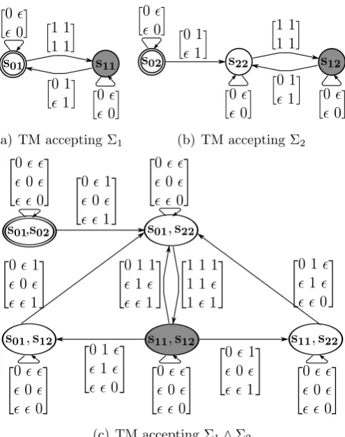
Example 2. We consider two sets of behaviors Σ1 and Σ2 defined on two
sets, V1 = {x, y} and V2 = {x, z} respectively, of variables with values
(a) TM accepting Σ1 (b) TM accepting Σ2
(c) TM accepting Σ1∧Σ2
Figure 5.1: Non-interoperable TMs
the variable value in the rest of the example. These behavioral sets are
expressed formally as follows. Let σi ∈ Σi and enumσi(vi) be the total
number of events on variable vi ∈ Vi in behavior σi where i ∈ {1,2} and
let k ≥1:
Σ1 :
σ1(x, k) = 2∗k −1
σ1(y, k) = k
enumσ1(y) = 2∗enumσ1(x)−1
Σ2 :
σ2(x, k) = 2∗k
σ2(z, k) =k
enumσ1(z) = 2∗enumσ1(x)
5.2. INTEROPERABLE TMS AND COMPOSITION SOUNDNESS
these behavioral sets can be organized in terms of successive reactions:
Σ1 :
x : 1 3 5 . . .
y : 1 2 3 4 5 6 . . .
Σ2 :
x : 2 4 6 . . .
z : 1 2 3 4 5 6 . . .
We use algebraic tag structure (N∪ {},6,+) and the tag piece structure described in Example 1 to model the behaviors in Σi as TMs where
def
=
−∞, the row and column designation orders are (x, y) in Figure 5.1(a),
(x, z) in Figure 5.1(b) and (x, y, z) in Figure 5.1(c). The initial states are
double-circled and the accepting states are shaded.
Tagging the shared variable x can depend on tagging non-shared
vari-ables y or z even though there is no real dependence between their tags.
Going from s01 to s11, TM 5.1(a) tags x and y simultaneously and equally.
It then can go back to s01, tagging only y and subsequently repeating the
tagging cycle at this state. TM 5.1(b) instead tags only z initially and
goes to s22. It then tags both x and z at the same time and goes to s12
where it again tags only z before returning to s22. It is easy to verify that
TM 5.1(a) and 5.1(b) accept the behavioral sets Σ1 and Σ2 respectively.
When composing them, the composed TM should not to accept any
be-havior since Σ1 ∧ Σ2 = ∅. Its set of accepted behavior is, however, not
empty as shown in Figure 5.1(c) because TM 5.1(a) can stay silent while
TM 5.1(b) is tagging z. The two TMs then synchronize and tag all
vari-ables simultaneously, after which they can go on tagging their own internal
variable.
Remarkably, the fact that TM composition is not sound was not
previ-ously observed in the homogeneous context [6]; since homogeneous
compo-sition is not sound, the same is true for heterogeneous compocompo-sition. The
composition, therefore building an abstraction. This may or may not be a
problem, depending on what is done with the models. For instance,
ver-ification of safety properties would be correct, albeit less precise. On the
other hand, the emergence of unexpected behaviors may adversely affect
the design process, where a refinement rather than an abstraction would
instead be more appropriate. It is therefore useful to look for conditions
that guarantee soundness. In our example, the dependency effects of
tag-ging non-shared variables on others, especially shared ones, are shown to
be the critical factor. The cause lies in the fact that in the applications of
tag pieces, the max tag evaluations for a shared variable can be different
even though the pieces are unifiable. It is therefore desirable to eliminate
such effects to make the composition sound. To this end, we propose an
interoperability condition to prevent TMs from producing such effects.
The intuition behind TM interoperability is that tagging shared
vari-ables should not depend on tagging non-shared varivari-ables. Because such
dependency is visible only internally inside components, it cannot be taken
into account in the composition. A set V ⊆ V is said to be locally indepen-dent in tag machine M = (V,T, S, s0, F, E), written lind(M, V), if tagging
v ∈ V depends only on tagging variables in V. If we define the following predicate
lind(µ, V) = (def ∀w ∈ V \V ,∀v ∈ V : µ(w, v) = ),
then the local independence of V in M is defined as
lind(M, V) = (def ∀(s, µ, s0) ∈ E : lind(µ, V)).
The interoperability betweenM1 and M2 is then formally defined as below.
Definition 9. Two TMs M1 and M2 are said to be interoperable, written M1 ./ M2, if their shared variables are locally independent in both TMs:
5.2. INTEROPERABLE TMS AND COMPOSITION SOUNDNESS
Interoperability behaves well under multiple composition.
Lemma 2. Let M1, M2, . . . Mn be n pair-wise interoperable TMs, where
n ≥ 2. If M is the composition of M1, M2, . . . Mn−1, then M ./ Mn.
Proof. We prove the lemma by inductive reasoning.
• The base case n = 2 is trivial.
• For the step case, we assume the lemma holds for k = n−1 and prove that it also holds for k + 1 = n. Let Vi be the variable set, µi a label
of Mi, µ the unification of µ1, µ2. . . , µn−1, T the fibered product of
T1,T2, . . . ,Tn−1 and V = V1 ∪V2. . .∪Vn−1.
It is easy to see that lind(µ, V ∩Vn) holds. Let w ∈ V \ (V ∩ Vn),
then it must be that w ∈ V and w /∈ Vn and so w ∈ Vj \Vn for some
1 ≤ j ≤ n−1. Likewise, let v ∈ V ∩ Vn, then v ∈ Vr ∩ Vn for some
1 ≤ r ≤ n−1. We show that µ(w, v) = T is true despite the choice of j and r.
i) Ifj andr can coincide, i.e.,j = r, then wandv can be in the same
variable set. Since Mr ./ Mn, by the interoperability definition it
is true that µr(w, v) = Tr and thus µ(w, v) = T.
ii) Otherwise, i.e.,j 6= r, thenw andv cannot be in the same variable
set and the wv−entries of the composed label µ are set to T, by the label composition rule in Section 5.1.
To show that lind(µn, V ∩Vn) holds, we consider w ∈ Vn \ (V ∩ Vn)
and v ∈ V ∩Vn. The latter means v ∈ Vr∩Vn for some 1 ≤ r ≤n−1.
The former means w ∈ Vn and w /∈ Vj for all 1 ≤ j ≤ n− 1 which
implies w ∈ Vn\Vr. This together with the interoperability Mn ./ Mr
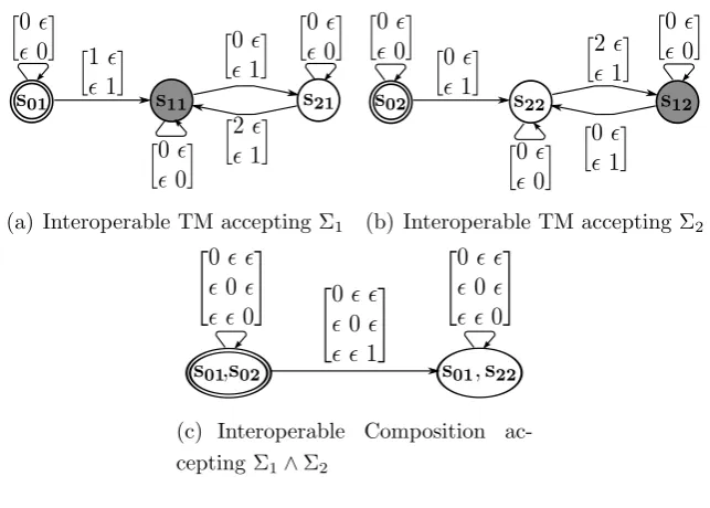
(a) Interoperable TM accepting Σ1 (b) Interoperable TM accepting Σ2
(c) Interoperable Composition
ac-cepting Σ1∧Σ2
Figure 5.2: Interoperable TMs
Example 3. We use the algebraic tag structure in Example 2 but restruc-ture the tag pieces so that they can represent any integer time increment
n∈ N.
µuv =
0 if u= v and µ has no event for v
n if u= v and µ has an event for v
otherwise
Interoperable TMs representing Σiare depicted in Figure 5.2(a) and 5.2(b).
Tagging the shared interface variablex is now made locally independent in
both machines, hence they can be composed interoperably. The composed
TM is shown in Figure 5.2(c) where no behavior can be accepted since
the accepting state is not reachable from the initial state. This is because
TM 5.2(a) has to stutter in s01 while TM 5.2(b) tags its internal variable
and moves to s22. The two TMs then have to stutter there forever since
only the stuttering labels 0 0 are unifiable.