Performance Optimisation of Dielectric Elastomer Generators

(1)

University of Trento

Department of Civil, Environmental and Mechanical

Engineering

DOCTORAL SCHOOL IN ENGINEERING OF

CIVIL AND MECHANICAL STRUCTURAL SYSTEMS

XXVIII CYCLE

Performance Optimisation

of

Dielectric Elastomer Generators

Author:

Eliana Bortot

Supervisor:

Prof. Massimiliano Gei

(2)

University of Brescia University of Padova University of Trieste University of Udine IUAV University of Venezia

Doctoral School in

Engineering of Civil and Mechanical Structural Systems

XXVIII cycle

Head of the Doctoral School:

Prof. Davide Bigoni, University of Trento (Italy)

Final examination: 17/12/2015

Board of Examiners:

Prof. Nicola Pugno, University of Trento (Italy)

(3)

“Non esiste una dignità della ricerca, perché nessuno può dire con sicurezza che una data ricerca non serve nè servirà mai a nulla. [...] Possiamo solo fabbricare mattoni, mattoni universali, con cui sia possibile fare qualsiasi cosa. Possiamo farci case, torri, ospedali, e persino fabbriche di mattoni. Ed è nostro dovere farli solidi, più solidi possibile, affinché le torri che edificheremo con quei mattoni possano arrivare più in alto possibile, e durare oltre le nostre vite.”

“It is impossible to set a worthiness upon a scientific research, because of the lack of certainty that a given research is definitely needed and useful. [...] What we can do is just to make bricks, universal bricks, with which it would be possible to do anything. We can build houses, towers, hospitals, and even brick factories. And our duty is to make them strong, the stronger the better, so that the towers which we are going to build with those bricks could reach the maximum heights and last beyond our lives.”

Marco Malvaldi

(4)

(5)

Summary

A Dielectric Elastomer Generator (DEG) is an electromechanical transducer, basically a highly deformable parallel-plate capacitor, made up of a soft DE membrane coated with two compliant electrodes on its opposite surfaces. This device is able to convert mechanical work, emanating from its interaction with the environment, into electrical energy. The capacitance depends on the deformation undergone by the membrane, and its variability can be exploited to extract electric energy by (i) initially stretching, (ii) then charging the capacitor, (iii) subsequently releasing the stretch and finally (iv) harvesting the charge at a higher electric potential.

The optimisation procedure for a load-driven soft planar DEG is presented, assuming hyperelastic and ideal dielectric behaviour. The DEG undergoes the ideal four-stroke electromechanical cycle previously described and its performance is evaluated on the basis of the energy extracted during a cycle and of the efficiency, defined as the ratio of the harvested energy on the total invested energy. The amount of extracted energy is limited due to possible failures of the device, which are, in the most general case, electric breakdown, material rupture, buckling-like instabilities due to loss of the tensile stress state and electromechanical instability. These failure mechanisms determine the allowable state region for the generator. Hence, in order to identify the best cycle that complies with these limits, a constrained optimisation problem is formulated and the generator performance is estimated. For the different loading cases examined, namely equibiaxial stress state and plane strain, numerical results show, as expected, a critical dependence of the harvested energy on the ultimate stretch ratio and, against expecta-tions, a universal limit on the dielectric strength of the DE membrane beyond which the optimal cycle is independent of this parameter. Thus, there is an upper bound on the harvested energy, which depends only on the ultimate stretch ratio.

In addition to the simple parallel-plate configuration, an annular DEG deforming out-of-plane has been analysed. In this configuration the generator is made up of an annular membrane constrained at the boundary by a rigid ring and at the centre by a rigid plate, on which an external force is applied. Due to the loading, the membrane deforms non-homogeneously out-of-plane. In order to avoid loss of the tensile stress state, electric breakdown and electromechanical instability, the applied voltage is controlled, thereby limiting the maximum voltage and keeping the maximum stretch in an admissible range. Numerical results show that the prestretch of the membrane is crucial for an effective behaviour of the device. In fact, the unprestretched generator performs poorly with regard to both energy and efficiency. A small prestretch, of approximately 5%, ensure a sixfold improvement in the gained energy and a fivefold increment in efficiency. The performance of the generator is evaluated for different values of the applied load and

(6)

decreases. Hence, for an out-of-plane DEG, the choice of the applied force is decisive to ensure a good trade-off among energy and efficiency. Moreover, a comparison of different DEG layouts demonstrates that the annular DEG can compete with the equibiaxial planar generator, in terms not only of efficiency, but also of harvested energy.

(7)

Acknowledgements

This dissertation collects the researches I carried out during the last three years as a Ph.D. student at the Dept. of Civil, Environmental and Mechanical Engineering of the University of Trento. I would like to take this opportunity to thank the people who have supported me during this work.

First of all, I would like to express my sincere gratitude to my advisor, Prof. Massimiliano Gei, for his patience, remarks, suggestions and encouragement throughout these years. I am deeply grateful to him for believing in me, working with him sincerely contributes to my scientific and personal growth.

I would like also to thank Dr. Roberta Springhetti, who provided me the opportunity to join the research on EAPs, for her unfailing presence.

I am deeply thankful to all members of the group of Solid and Structural Mechan-ics at the University of Trento: Prof. Davide Bigoni, Prof. Luca Deseri, Prof. Nicola Pugno, Prof. Andrea Piccolroaz, Dr. Francesco Dal Corso and Dr. Fiorella Pantano. I would like to thank all my current and former colleagues, in particular Dr. Luca Ar-gani, Dr. Federico Bosi, Dr. Aldo Madaschi, Dr. Diego Misseroni, Dr. Lorenzo Morini, Stefano Signetti, Pietro Pollaci, Summer Shazad, Costanza Armanini, Nicola Bordigon and Mirko Tommasini.

I am deeply indebted to Prof. Gal deBotton for his cooperation during these three years. His valuable suggestions and his friendly words of advice guided me through this research path since the beginning.

I would like to express my deepest gratitude to Prof. Andreas Menzel for his strong support, encouragement and his confidence in my work. I am also deeply grateful to the whole group of the Institute of Mechanics at TU Dortmund for their friendly and warm hospitality during my four-month stay in 2013 and for making me feel part of the ”family” even after: Prof. Jörn Mosler, Prof. Björn Kiefer, Dr. Thorsten Bartel, Dr. Guillermo D`ıaz Ort`ız, Dr. Krishnendu Haldar, Dr. Richard Ostwald, Dr. Tobias Waffenschmidt, Alexander Bartels, Rolf Berthelsen, Karsten Buckmann, Cèsar Polin-dara, Raphael Holtermann, Dinesh Kumar Dusthakar, Maniprakash Subramanian and the wonderful secretaries Tina McDonagh and Kerstin Walter.

Special thanks go to Prof. Ralf Denzer, former member of the Institute of Mechanics at TU Dortmund and now working at Lund University, for his constant support, for the scientific discussions and the friendly chats. His precious teachings and help have been decisive to the success of this work.

(8)

their patience, understanding and love this work would not have been possible.

Trento, December 2015

(9)

List of publications

The main results presented in this thesis have been published in the following publica-tions:

• Bortot, E., Springhetti, R., Gei, M. (2014) Enhanced soft dielectric composite generators: The role of ceramic fillers. Journal of the European Ceramic Society,

34(11), 2623-2632. doi:10.1016/j.jeurceramsoc.2013.12.014

• Springhetti, R., Bortot, E., DeBotton, G., Gei, M. (2014) Optimal energy-harvesting cycles for load-driven dielectric generators in plane strain. IMA Journal of Applied Mathematics,79(5), 929-946. doi:10.1093/imamat/hxu025

• Bortot, E., Denzer, R., Menzel, A., Gei, M. (2014) Analysis of a viscous soft dielec-tric elastomer generator operating in an elecdielec-trical circuit. Proceedings in Applied Mathematics and Mechanics,14 (1), 511-512. doi:10.1002/pamm.201410243

• Bortot, E., Springhetti, R., DeBotton, G., Gei, M. (2015) Optimization of load-driven soft dielectric elastomer generators. Procedia IUTAM,22, 42–51.

doi:10.1016/j.piutam.2014.12.006

• Bortot, E., Gei, M., DeBotton, G. (2015) Optimal energy harvesting cycles for load-driven dielectric elastomer generators under equibiaxial deformation. Mecca-nica,50(11), 2751-2766. doi:10.1007/s11012-015-0213-1

• Bortot, E., Denzer, R., Menzel, A., Gei, M. (2015) Analysis of a viscous soft dielec-tric elastomer generator operating in an elecdielec-trical circuit. International Journal of Solids and Structures. In press. doi:10.1016/j.ijsolstr.2015.06.004

• Bortot, E., Gei, M. (2015) Harvesting energy with an out-of-plane dielectric elas-tomer generator. Proceedings in Applied Mathematics and Mechanics, 15 (1), 379–380. doi:10.1002/pamm.201510180.

• Bortot, E., Gei, M. (2015) Harvesting energy with load-driven dielectric elastomer annular membranes deforming out-of-plane. Extreme Mechanics Letters,5, 62-73. doi:10.1016/j.eml.2015.09.009

Other results obtained during the Ph.D. course are reported in the following publications:

• Gei, M., Springhetti, R., Bortot, E. (2013) Performance of soft dielectric laminated composites. Smart Materials and Structures,22(10), 104014.

doi:10.1088/0964-1726/22/10/104014

(10)

(11)

List of Figures

1.1 Examples of DE energy harvesters: a) heel-strike generator tested by SRI international [10] and b) polymeric oscillating water column developed in the PolyWEC project [61]. . . 2

2.1 Reference and deformed configurations of a soft planar DE generator with undeformed dimensions (l0×l0×h0): as a result of the deformation, the

current dimensions arel1 =l0λ1,l2=l0λ2 andh=h0λ3. . . 5

2.2 The load-driven harvesting cycle plotted on the a) mechanical and b) elec-trical planes and c) illustration of the four strokes with a service battery at the right and a storage battery at the left; the illustrations in c) are referred to the initial states of each individual stroke. . . 15

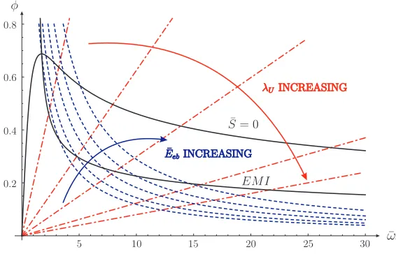
2.3 Failure envelopes for a plane-strain loaded DEG on the electrical ¯φ–¯ω0

plane for increasing values of the electric breakdown strength ( ¯Eeb =

0.4,0.6,0.8,1) and of the ultimate stretch (λU = 1.5,2,2.5,3,3.5). . . 18

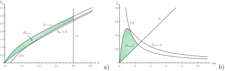
2.4 Failure envelopes at ¯Eeb = 0.8 and λU = 3 on the a) mechanical ¯S11–λ

and b) electrical ¯φ–¯ω0 planes for a plane-strain loaded DEG. . . 19

2.5 Failure envelopes for an equibiaxially loaded DEG on the electrical ¯φ– ¯

ω0 plane for increasing values of the electric breakdown strength ( ¯Eeb =

1.09,1.2,1.3,1.5,1.7) and of the ultimate stretch (λU = 1.5,2,2.5,3,3.5). . 21

2.6 Failure envelopes at ¯Eeb = 0.8 andλU = 3 on the a) mechanical ¯S–λand

b) electrical ¯φ–¯ω0 planes for an equibiaxially loaded DEG. . . 21

3.1 Reference and deformed configurations of a soft planar DE generator with undeformed dimensions (l0×l0×h0) subjected to a plane-strain loading:

as a result of the deformation, the current dimensions arel1=l0λ,l2 =l0

and h=h0λ−1. . . 25

3.2 Region of admissible state for a plane-strain loaded DEG with ¯Eeb= 0.8,

λ∗= 1.667 and ˆω0 = 2.828 on the a) mechanical and b) electrical planes. . 29

3.3 Optimal cycles on the mechanical and electrical planes for λU = 3 and:

a) ¯Eeb = 0.6 and b) ¯Eeb ≥0.8263. . . 31

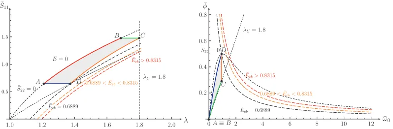
3.4 Optimal cycles on the mechanical and electrical planes for λU = 1.8 and

¯

Eeb ≥0.6889. . . 32

3.5 A universal plot for planar plane-strain load-driven DEGs. The abscissa and the ordinate of the plot correspond to the electromechanical limits of the film λU and ¯Eeb, respectively. The dark-blue curve divides the

space of materials parameters into two sections, depending on the mode of failure at point D of the optimal harvesting cycle. Beyond the light-blue curve the electric breakdown becomes unimportant in the definition of the allowable state region. The dark-blue dashed curve is related to the analytical prediction (3.14). . . 33

(16)

3.6 Approximation of the cycle area through a rectangle whose height is equal to the potential differenceδφ¯among the loss of tension (S22= 0) and the

ultimate stretch λU curve. . . 34

3.7 Values of the electric breakdown strength Eeb [MV/m] as a function of

the shear modulus µand of the relative dielectric permittivity r for the

best performance in terms of: a) efficiency,λU = 1.546 (MΛU) and ¯Eeb=

0.5929, and b) energy, λU = 3 (HΛU) and ¯Eeb = 0.8263. . . 37

4.1 Reference and deformed configurations of a soft planar DE generator with undeformed dimensions (l0×l0×h0) subjected to equibiaxial loading: as

a result of the deformation, the current dimensions are l=l1 =l2 =l0λ

and h=h0λ−2. . . 41

4.2 Region of admissible state for an equibiaxially loaded DEG with ¯Eeb =

1.0912, λ∗ = 1.259, λ∗∗ = 1.739, ˜ω0 = 15.642 and ˆω0 = 26.981 on the a)

mechanical and b) electrical planes.. . . 45

4.3 Optimal cycles for λU = 3 and: a) ¯Eeb = 0.9, b) ¯Eeb = 1.038, c) ¯Eeb =

1.091, and d) ¯Eeb ≥1.396. . . 48

4.4 Optimal cycles for λU = 2.1 and: a) ¯Eeb <1.091 and b) ¯Eeb≥1.091. . . . 50

4.5 Optimal cycles for λU = 1.8 and: a) ¯Eeb <1.091 and b) ¯Eeb≥1.091. . . . 50

4.6 A universal plot for planar equibiaxial load-driven DEGs. The abscissa and the ordinate of the plot correspond to the electromechanical limits of the filmλU and ¯Eeb, respectively. The dark-blue and orange curves divide

the space of materials parameters into sections depending on the mode of failure at point D of the optimal harvesting cycle. Along the solid-dotted dark-blue curve we distinguish between the high, the moderate and the low ultimate stretch regions. Uniquely below the dark-blue curve, the failure depends on the electrical breakdown limit. Along the solid light-blue curve we distinguish between Case a and Case b, so that above this curve the electrical breakdown does not participate in the definition of the allowable state region. . . 52

4.7 Values of the electric breakdown strength Eeb [MV/m] as a function of

the shear modulus µand of the relative dielectric permittivity r for the

best performance in terms of: a) efficiency, for λU = 1.563 (MΛU) and

¯

Eeb = 1.091 and b) energy, forλU = 3 (HΛU) and ¯Eeb= 1.396. . . 55

4.8 Universal design curve for planar equibiaxial load-driven DEGs already introduced in Fig. 4.6: electromechanical characteristics of the three com-posites, black shapes, and of their PDMS matrices, white shapes. . . 62

4.9 Optimal cycle for (I) the pure PDMS and (II) the PDMS–%10PMN–PT composite, on the A) mechanical and B) electrical planes, in the case λU = 1.8. With respect to the EB influence on the optimal cycle, both

materials appertain to subregion (iii) (cf. e.g. Fig. 4.8). With respect to the EB influence on the admissible state region, the pure PDMS is related to Case b, whereas the composite pertains to Case a. . . 64

4.10 Optimal cycle for (I) the pure PDMS and (II) the PDMS–%10PMN– PT composite, on the A) mechanical and B) electrical planes, in the case λU = 3.0. With respect to the EB influence on the optimal cycle, the pure

(17)

List of Figures xvii

5.1 Sketch of the periodic four-phase cycle for the investigated electroactive membrane generator (phases IV and I coincide): a) membrane configu-rations; b) mechanical force (F)–out-of-plane displacement (u) plane; c) multi-membrane device subjected to a total force Ftot. . . 71

5.2 Configurations of the annular membrane generator: a) undeformed, b) pre-stretched and c) deformed.. . . 72

5.3 The investigated harvesting cycle: a) illustration of the four strokes along the I–II–I path with a service battery at the right and a storage battery at the left b) plot of the cycle on the electricalQ–φplane and on the mechan-icalF–u plane. The measure of the area of the cycle, on both planes, is equal to the modulus of the harvested energy,|Hg|. The light-grey shaded

areas represent the electrical and the mechanical work invested into the conversion process. . . 77

5.4 Influence of the prestretch on the performance of a generator withre 0/ri0=

2. Plot on the electrical φ–Q plane of the optimal cycle for different prestretch values, namelyλpre= 1, 1.05, 1.1, 1.25, 1.5 and 2, andFmax=

90 N. The relevant failure mode is indicated below the prestretch label. . 79

5.5 Influence of the prestretch λpre on the performance of a generator with

re₀/r₀i = 2, Fmax = 90 N: a) gained energy per unit mass ˆHg and b)

efficiencyη. The failure mode in the relevant prestretch range is reported below the horizontal axis. . . 80

re₀/r₀i = 2, F_max = 90 N: a) maximum stretch λmax and b) maximum

current electric field Emax. The failure mode in the relevant prestretch

range is reported below the horizontal axis. . . 81

5.7 Influence of the radius ratiore₀/r₀i on the performance of the generator for different prestretches: a) gained energy per unit mass ˆHgand b) efficiency

η.. . . 83

5.8 Influence of the maximum applied load F_max on a) the efficiency η and b) the gained energy per unit mass ˆHg of a generator with r0e/ri0 = 2. A

dot at the end of a curve indicates that one stretch in the membrane has reached the ultimate value λmax =λU = 4 (in all casesλ1 =λmax). . . 84

6.1 Soft dielectric elastomer generator: a) reference configuration and b) scheme of the equivalent circuit diagram. . . 90

6.2 Scheme of the electrical circuit in which the dielectric elastomer generator operates.. . . 91

6.3 Viscoelastic behaviour of VHB-4910: stress response at different strain rates as obtained from parameter identification. Dots: experimental data based on experiments by Tagarielli et al. [58]; solid lines: simulated data. 95

6.4 Dielectric permittivity of VHB-4910 at different equibiaxial stretches for two representative frequencies ¯f as obtained from parameter identification based on experiments by Tagarielli et al. [58]. . . 96

6.5 Plot of loading cycles of a DEG a) in the mechanical S–λand b) in the electricalφC+φRs–Qplanes at different initial timesti, namely 10, 50, 100

and 200 seconds. Model VC, λo= 3.0,Λ = 0.50, f = 0.1 Hz, Rext = 0.1

(18)

6.6 Plot of loading cycles of a DEG a) in the mechanical S–λand b) in the electrical φ_C +φRs–Q planes at different initial times ti, namely 10, 50,

100 and 200 seconds. Model VC,λo = 3.0,Λ= 0.50,f = 1 Hz,Rext= 0.1

GΩ. . . 101

6.7 Plot of the viscous dissipation Dv and the leakage dissipation DRi at

different frequencies f. Model VC, λo = 3.0,Λ= 0.50,Rext= 0.1 GΩ. . . 101

6.8 Plot of the efficiencyη(Rext, f) for the three different material models: a)

hyperelastic, HYP, b) viscoelastic, VC, and c) electrostrictive viscoelastic, VE. Equi-biaxial loading conditions with λo = 3.0; Λ = 0.50, Λ = 0.25

and Λ= 0.10. . . 104

6.9 Plot of the efficiency η versus a) frequency f at Rext = 1 GΩ, and b)

external resistance Rext at f = 1 Hz. Equi-biaxial loading conditions

withλo = 3.0;Λ= 0.50, 0.25, 0.10. Dashed, continuous and dotted lines

are referred respectively to HYP, VC and VE models. . . 105

6.10 Plot of the efficiency η versus frequency f for two values of the mean value of the oscillation stretch λo= 1.8 and λo = 3. Equi-biaxial loading

conditions with Rext= 1 GΩ, VC model. . . 106

6.11 Plot on the electrical ¯φ–¯ω0 plane of the failure envelope for different values

of the mean stretch λo. Solid lines are referred to the VC model, dashed

lines to the HYP model. . . 108

6.12 Plot on the electrical ¯φ–¯ω0plane of the a) loss of tensile state and b)

elec-tromechanical instability curves for different values of the mean stretch, namely λo = 1.8,3,4. Solid lines are referred to the VC model, dashed

lines to the HYP model. . . 109

6.13 Plot of the cycle on the electrical plane for different values of the product f Rext, at λo = 3 and Λ = 0.695. The failure curves are represented by

dashed black lines for the HYP model and by solid black lines for the VC model. . . 110

6.14 Plot of the maximal oscillation amplitudeΛmax as a function of the

prod-uctf Rextforλo= 3. . . 111

6.15 Plot of the efficiencyη(Rext, f) for an external resistanceRext=1 GΩ and

λo = 3.0, Λ = 0.50 and Λ = 0.25. Dashed, continuous and dotted lines

are referred respectively to HYP, VC and VE models. . . 112

A.1 Nelder-Mead method: reflection of the simplex. . . 121

A.2 Nelder-Mead method: expansion of the simplex.. . . 121

A.3 Nelder-Mead method: contraction of the simplex a) outside and b) inside. 121

(19)

List of Tables

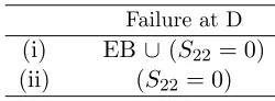
3.1 Classification of the optimal cycles for plane-strain load-driven DEGs, according to the relevance of the electric breakdownEeb on the failure at

D, cf. Fig. 3.5. . . 30

3.2 Relevant numerical values for optimal cycles associated with a DEG with λU = 3 and different values of ¯Eeb. . . 32

3.3 Relevant numerical values for optimal cycles associated with a DEG with λU = 1.8 and different values of ¯Eeb. . . 33

3.4 Electromechanical properties ensuring the best performance in terms of efficiency and harvested energy for a plane-strain load-driven DEG.. . . . 35

3.5 Physical properties assumed for the elastic dielectrics. . . 38

3.6 The harvested energy-density µHg, activation electric potential per unit

referential thickness ∆φ/h0 and material classification M-C, determined

for the optimal cycles according to the dielectric strength limits and the maximal stretch ratios λC determined for the maximum stresses Smax. . . 38

4.1 Classification of the optimal cycles for equibiaxial load-driven DEGs, ac-cording to the relevance of the electric breakdown Eeb on the failure at

D, cf. Fig. 4.6. . . 47

4.2 Relevant numerical values for optimal cycles associated with a DEG with λU = 3 and different values of ¯Eeb. . . 49

4.5 Relevant numerical values for optimal cycles associated with a DEG with λU = 1.4 and for different values of ¯Eeb. . . 52

4.6 Electromechanical properties ensuring the best performance in terms of efficiency and harvested energy for an equibiaxial load-driven DEG. . . . 54

4.7 Physical properties and electric breakdown parameters for the rigid elec-trode configuration. . . 56

4.8 Electric breakdown data for the two elastomers at different ultimate stretches λU, see [60]. . . 56

4.9 Data for DEGs with two MΛU elastomers and two configurations: ˆHg=

µHg/ρ, harvested energy density per unit mass, ∆φ/h0, activation electric

potential per unit referential thickness,η, efficiency, M-C, material classi-fication according to Fig. 4.6, ˆHmax=µHmax/ρ, theoretically achievable

energy,ζ, effectiveness;n, number of 1 mm thick layers required to sustain 1 kN atλU,nH˜g, total harvested energy by the multi-membrane DEG. . . 57

(20)

4.10 Data for DEGs with two HΛU elastomers and two configurations: ˆHg =

µHg/ρ, harvested energy density per unit mass, ∆φ/h0, activation electric

potential per unit referential thickness,η, efficiency, M-C, material classi-fication according to Fig. 4.6, ˆHmax=µHmax/ρ, theoretically achievable

energy,ζ, effectiveness;n, number of 1 mm thick layers required to sustain 1 kN atλU,nH˜g, total harvested energy by the multi-membrane DEG. . . 58

4.11 Sets of parameters for the ceramic–polymer composites analyzed. . . 60

4.12 Sets of parameters for the three PDMS involved in the ceramic–polymer composites. . . 61

4.13 Material classification M-C, according to Fig. 4.8, and generated energy-density per unit shear modulus Hg for the selected harvesting cycles for

the composite material a) and its matrix. . . 63

4.14 Material classification M-C according to Fig. 4.8, generated energy per unit volume µHg, required voltage ∆φ(inside square brackets) and

per-centage gain for the selected harvesting cycles allowed by the composite material a) over its matrix. . . 63

the composite material b) and its matrix. . . 65

4.16 Material classification M-C according to Fig. 4.8, generated energy per unit volume µHg and per unit mass ˆHg, required voltage ∆φ for the

selected harvesting cycles (inside square brackets) and percentage gain allowed by the composite material b) over its matrix. . . 66

the composite material c) and its matrix. . . 67

4.18 Material classification M-C according to Fig. 4.8, generated energy per unit volume µHg, required voltage ∆φ for the selected harvesting cycles

(inside square brackets) and percentage gain allowed by the composite material c) over its matrix. . . 67

5.1 Electromechanical properties of VHB-4910. . . 78

re₀/r₀i = 2. Gained energy per unit mass ˆHg, efficiencyη, supplied voltage

∆φand obtained voltage jumpφD−φC are reported. For each examined prestretch the failure mode experienced by the device is listed. Further-more, the improvement in the gained energyδHˆg and in the efficiency δη

with respect to the unprestretched case (λpre= 1) are quantified. . . 82

5.3 Influence of the radius ratio on the generator performance: internal ra-dius ri

0 (re0 = 500 mm), and maximum applied load Fmax. For the best

performance of the generator, the prestretch λpre, the gained energy per

unit mass ˆHg, the efficiency η, the applied voltage ∆φ and the obtained

voltage jump φD₋_φC _{are reported.} _{. . . 83}

(21)

List of Tables xxi

5.5a Performance comparison of devices made up of two different materials working at maximum efficiency. Left-hand and central parts of the table refer to the behaviour of a single membrane. The right-hand side of the table reports the performance of multi-membrane systems subjected to a total maximum force F_tot = 34 kN: n, number of layers required; n|Hg|,

total energy harvested. . . 86

5.5b Performance comparison of devices made up of two different materials working at maximum energy. Left-hand and central parts of the table refer to the behaviour of a single membrane. The right-hand side of the table reports the performance of multi-membrane systems subjected to a total maximum force Ftot = 34 kN: n, number of layers required; n|Hg|,

total energy harvested. . . 86

5.6a Performance comparison atλmax = 2.4 for different prototype generator

configurations, acrylic material properties (VHB-4910) . . . 87

5.6b Performance comparison atSmax= 70 kPa for different prototype

gener-ator configurations, acrylic material properties (VHB-4910) . . . 87

6.1 Mechanical material parameters. . . 95

6.2 Electrical and coupling material parameters.. . . 96

6.3 Energy produced by the generator and mechanical work invested at two different frequencies, f = 0.1 Hz and f = 1 Hz, computed after 200 s for the three material models considered: λo = 3, Λ = 0.50, 0r = 6.4,

Rext= 0.1 GΩ. The reference volumeV0 is given by l02h0. . . 102

6.4 Maximal oscillation amplitude Λmax achievable in an equibiaxial test

without inducing in-plane negative stresses. Model VC, Rext = 0.1 GΩ,

f = 1 Hz. . . 102

6.5 Energy produced by the generator and mechanical work invested for the three selected amplitudes Λ = 0.10, Λ = 0.25 and Λ = 0.50, computed after 200 s for the VC model: λo = 3,f = 1 Hz,0r= 6.4,Rext= 0.1 GΩ.

(22)

(23)

Abbreviations

DE Dielectric Elastomer

DEA Dielectric ElastomerActuator

DEG Dielectric ElastomerGenerator

EAP Electro ActivePolymer

CCTO calcium copper titanateCaCu3Ti4O12

PDMS Poly–DiMethyl–Siloxane

PMN–PT lead magnesium niobatePb(Mg₁_/₃Nb₂_/₃)O3 – lead titanatePbTiO3

PZT lead zirconate–titanatePb[Zr1−xTix]O3

(24)

(25)

Physical Constants

Vacuum Permittivity 0 = 8.854 187 817×10−12 Fm−1

Elementary Charge qe = 1.602 176 53×10−19 C

(26)

(27)

Symbols

˜

Hmax theoretically achievable energy [J]

˜

Hg harvested energy [J]

˜

Hi invested energy [J]

Hmax theoretically achievable energy-density per unit shear modulus dimensionless

Hg harvested energy-density per unit shear modulus dimensionless

Hi invested energy-density per unit shear modulus dimensionless

ˆ

Hg harvested energy per unit mass [J kg−1]

ˆ

Hi invested energy per unit mass [J kg−1]

P current polarisation [C m−2]

E current electric field [V m−1_]

E0 nominal electric field [V m−1]

D current electric displacement [C m−2_] D0 nominal electric displacement [C m−2]

Q electric charge [C]

i electric current [A]

Eeb current electric breakdown strength [V m−1] X material position vector

x spatial position vector

F deformation gradient dimensionless

S Piola stress [Pa]

f_e electrical body force [N m−3]

f mechanical body force [N m−3]

C Cauchy–Green tensor

Cvα internal variable tensor

F force vector [N]

(28)

T temperature [K]

f frequency [Hz]

T period [s]

W strain-energy function based onE0, Gibbs potential

W strain-energy function based onD0, Helmholtz potential

Rs electric resistance [Ω]

Ri electric resistance [Ω]

Rext electric resistance [Ω]

C electric capacitance [F]

Pin input power [W]

Pout output power [W]

Ein input electrical energy [J]

Eout output electrical energy [J]

∆E energy produced by the generator [J]

l0 nominal side length [m]

l current side length [m]

h0 nominal thickness [m]

h current thickness [m]

r0 nominal radius [m]

r current radius [m]

u maximum transverse displacement [m]

r₀i nominal inner radius [m]

r₀e nominal external radius [m]

A0 reference undeformed area [m2]

A current area [m2]

V0 reference undeformed volume [m3]

V current volume [m3]

J volume ratio dimensionless

µ shear modulus [Pa]

ρ0 density in the undeformed configuration [kg m−3]

(29)

Symbols xxix

permittivity [F m−1]

βα proportionality factor among the shear modulus dimensionless

of the α Maxwell element and the long term one ˙

Γα material parameter, inverse of the viscosity of the [s−1 Pa−1]

α Maxwell element

Φ(X) electrostatic potential

ω0 referential charge density [C m−2]

φ voltage [V]

¯

ω0 referential charge density dimensionless

¯

φ voltage dimensionless

η efficiency dimensionless

ζ effectiveness dimensionless

λ principal stretch dimensionless

λpre prestretch dimensionless

λv viscous principal stretch dimensionless

λo oscillation mean value dimensionless

Λ oscillation amplitude dimensionless

ψ angular frequency [rad s−1_]

(30)

(31)

In memory of Prof. Federico di Varmo

(32)

(33)

Chapter 1

Introduction

In recent years, the urgency of energy from renewable resource has become increasingly crucial, thereby giving new impulse to the development of new concepts and modern techniques. Among the various energy harvesting technologies, a particularly promis-ing one is based on soft dielectric elastomers (DEs) [1, 9, 10, 38, 44]. Being reliable, quick responsive, light, cheap and involving a few moving parts, such electro-mechanical transducers are suitable for different applications, allowing energy extraction from sea waves, wind gusts, human gait and other natural sources of mechanical work, see for example Figs. 1.1a and1.1b.

A Dielectric Elastomer Generator (DEG) is basically conceived as a highly stretchable parallel-plate capacitor with variable capacitance, able to produce electrical energy con-verting the mechanical work done by an external oscillating load. This device is simply made up of a soft DE membrane, whose upper and lower surfaces are treated so as to act like compliant electrodes. The capacitance depends on the current geometry of the dielectric film, therefore it changes as a consequence of the stretch and release of the membrane induced by its interaction with the external environment. This significant ca-pacitance variability can be exploited to extract electrical energy through a four-stroke cycle where (i) an initial, relatively slow, stretching of the elastomeric film induced by the rising force is followed by (ii) a fast charging phase. Then, (iii) the capacitor is relaxed due to the slow release of the load and (iv), finally, the charge is harvested at high electric potential and at low force.

Different configurations and harvesting cycles have been proposed in the literature es-sentially involving three charging–discharging strategies, distinguished by the electrical variable - among electric field, charge and voltage - to be kept constant along both the stretching and the contracting phases induced by the mechanical force [39]. In this work, differently from others [25,30,36], we assume that the mechanical load and the electric

(34)

a)

b)

Figure 1.1: Examples of DE energy harvesters: a) heel-strike generator tested by SRI international [10] and b) polymeric oscillating water column developed in the PolyWEC

project [61].

charge are alternately held constant during the cycle. This means that the stretching and contracting phases occur at constant charge, for example when the system is electri-cally isolated (open-circuit condition), while charging and harvesting phases take place at stationarity points of the loading function.

The amount of extracted energy is limited due to possible failures of the dielectric membrane, which are, in the most general circumstances, electric breakdown, material rupture, buckling-like instabilities, due to loss of the tensile stress state, and electrome-chanical instability [5, 49]. These failure mechanisms determine the allowable state region for the generator [37].

(35)

Chapter 1. Introduction 3

showed that significant improvements in the generated energy density can be achieved using an equibiaxial mechanical loading configuration accounting also for viscoelasticity. Vertechy et al. [61] proposed a polymer-based oscillating-water-column energy converter (Fig. 1.1b).

This monograph is dedicated to a systematic investigation of the performance optimi-sation of DEGs in the framework of the nonlinear theory of electro-elasticity. The main goal of this research is the identification, by means of a numerical analysis, of those cycles able to produce the maximum energy fulfilling the constraints associated with the various failure modes.

After recalling, in Chap. 2, the basic elements of continuum electro-mechanics and the working principles of DEGs, the optimisation procedure for a planar load-driven soft DEG is presented, assuming isotropic hyperelasticity and ideal dielectric behaviour, for plane-strain (Chap.3) and equibiaxial (Chap.4) loading modes. In order to identify the best cycle that complies with the limits dictated by the failure envelope, a constrained optimisation problem is formulated and the generator performance is estimated on the basis of both the energy extracted during a cycle and the efficiency, i.e. the ratio of the harvested energy on the total invested energy. For the two loading cases exam-ined, in Chaps.3and 4, numerical results for different stretch regimes and performance comparisons for various soft DEs commercially available are presented.

The chosen loading modes are justified on the grounds that plane-strain condition simu-lates the effect of transverse constraint due to stiff fibres [40] or a supporting frame, while equibiaxial condition can be produced by an external agent in a mechanism involving the expansion of a dielectric balloon due to internal pressure [12,48,53].

(36)

with different electromechanical properties are investigated and various DEG geometries, under similar stress/stretch conditions, are compared.

Dielectric elastomers, as all polymers, are affected by time-dependent effects, hence the conservative hypothesis appears to be not completely realistic. Indeed, a predicting model for soft DEGs must include an accurate model of the electro-mechanical behaviour of the elastomer filling, the variable capacitor and of the electrical circuit connecting all the device components. To this end, the ideality assumption of the material and of the cycle has to be removed. Hence, in Chap. 6, a complete framework for a reliable simulation of soft energy harvesters is presented for a soft electro-viscoelastic DEG, mechanically excited by a periodic stretch and integrated in an electrical circuit for energy harvesting.

(37)

Chapter 2

Dielectric elastomer generators:

theory

A dielectric elastomer generator is an electro-mechanical transducer able to convert mechanical to electric energy. The basic idea behind its operating principle consists in varying its capacitance with the deformation, hence this device can be regarded as a highly deformable soft capacitor.

In the simplest framework, a three-dimensional soft dielectric elastomer generator is made up of a dielectric elastomer membrane whose surfaces are treated so as to act like compliant electrodes and whose initial volume is V0 =l0×l0×h0 in the reference

undeformed configuration. Essentially, this DEG is a parallel-plate soft capacitor.

_

_ _ _ _ _ _ _ _ _ _ + + + + + + + + +

_

+ + + + + + + + + + + + + + + + + +

_ _

Figure 2.1: Reference and deformed configurations of a soft planar DE generator

with undeformed dimensions (l0×l0×h0): as a result of the deformation, the current dimensions arel1=l0λ1, l2=l0λ2 andh=h0λ3.

We assume that the dielectric membrane is homogeneous, isotropic and incompressible. The membrane is stretched from the undeformed to the current configuration by a com-bination of (i) a mechanical in-plane force F induced by the environment, which is the primary source of energy invested into the system, and (ii) an electric field generated by

(38)

a voltageφapplied between the stretchable electrodes. We note that an alternative way to electrically excite the deformation is by depositing electrical charge on the opposite surfaces of the specimen [33]. However, in this work we do not consider this alternative, since, from a practical viewpoint, it is more convenient to impose the required electric potential between the electrodes.

Neglecting fringing effects and assuming isotropy, the electromechanical deformation undergone by the membrane is homogeneous and can be represented by the deformation gradientF = diag(λ1, λ2, λ3), whereλ1,λ2 and λ3 are the principal stretch ratios along

the directions (e1,e2,e3), see the coordinate systems in Fig.2.1. Outside the capacitor

the electric field vanishes, and the uniform electric field induced by the applied electric potential inside the membrane has only a component alonge3, namelyE = [0,0, E]T.

2.1

Theoretical background: kinematics and governing

equa-tions

For the motion of the material body considered, we assume the existence of a sufficiently smooth mapping ϕ(X, t) transforming the position vector X of a material particle in the undeformed configuration B₀ to its spatial position x = ϕ(X, t) in the current configuration Bt at time t (see e.g. Fig. 2.1). Hence, the deformation gradient tensor

is given by F = Gradϕ, where the gradient is taken with respect to the reference configuration B0. The local volume ratio is the Jacobian of the deformation gradient

tensor J = detF with J = 1 for incompressible materials. The right Cauchy-Green tensor is defined byC =FTF and, thus, we formally introduce here the stretches λ1,

λ2,λ3, as the square roots of the eigenvalues of C such thatJ =λ1λ2λ3.

The quantities of interest to define the current electrostatic state of the dielectric are the electric field E, the electric displacements D and the polarisation P in Bt, linked

by the relation

D =oE +P,

where0 is the dielectric permittivity of vacuum (0 = 8.854 pF/m).

Electromagnetic interactions are governed by Maxwell’s equations. We assume through-out this work that (i) the hypotheses of electrostatics hold true and that (ii) free currents and free charges are absent. Therefore, Maxwell’s equations in local form with respect to the current configurationBt reduce to

(39)

2.1 Theoretical background: kinematics and governing equations 7

or with respect to the reference configurationB0 to

CurlE0 =0, DivD0= 0, (2.2)

where the following nominal fields

E0 =FTE, D0 =JF−1D, (2.3)

are naturally introduced. See [5] for the exact derivation.

The notation used in Eqs. (2.1) and (2.2) is such that the uppercase letters indicate operators acting onB0, e.g. Grad, Div, Curl, whereas lowercase letters refer to operators

defined in the configurationB_t, e.g. grad, div, curl. Eq. (2.2)1 implies that the electric

field is conservative, i.e.

E0(X) =−GradΦ(X), (2.4)

where Φ(X) is the electrostatic potential. At the boundary ∂B₀, the electric field and the electric displacement must fulfil the jump conditions

N0×[[E0]] =0, [[D0]]·N0=−ω0, (2.5)

where ω0 is the charge density per unit reference electrode surface, [[f]] = fa−fb is

the jump operator and where N0 denotes the outward referential unit normal vector, pointing fromatowardsb.

Considering the electric field uniform, as for the parallel-plate DEG sketched in Fig.2.1, the nominal electric field can be expressed as E0 = φ/h0 with φ = |∆Φ| representing

the voltage between the electrodes andh0 being the reference thickness of the film. The

electric field is similarly defined as E =φ/h, where the current thickness h is given by

h = h0λ3. The nominal charge density ω0 can analogously be referred to its current

counterpart ω given the charge Q = ωA = ω0A0, where the current area of the film

surfaces A is related to the area in the reference configuration A0 as A = A0λ1λ2,

therefore,ω =ω0λ1λ2. For the planar capacitor, Eq. (2.5)2 and Eq. (2.3)2 show thatω

and ω0 correspond to the absolute values of the current electric displacementD and of

the nominal electric displacementD0, respectively.

In the quasi-static case, the local form of the balance of linear momentum in Bt

corre-sponds to

divσ+f_e+ρf=0, (2.6)

(40)

inertia term is neglected in both rate-independent and rate-dependent quasi-static cases, since its contribution is negligible for the frequency range investigated in this work, as will be explained later in Chap.6. For the problem at hand, the electric body force can be specified as follows

f_e= gradE P.

Moreover, the Cauchy stress tensor σ is generally non-symmetric, whereas the total stress tensor

τ =σ+E ⊗D −1

20[E ·E]I,

as introduced in e.g. [15, 27, 43, 45], turns out to be symmetric. The second-order identity tensor is denoted byI. In this way, it is possible to rewrite the balance of linear momentum as

divτ+ρf=0.

Note that the form of the electric body force f_e is not the only possible one, since the choice of other sets of the electrical and mechanical variables can fit the general theory based on the total stress, see e.g. [8].

The total Piola-type stress tensor S is defined as S =JτF−T, so that the local refer-ential form of the balance of linear momentum can be written as

DivS+ρ0f=0,

where ρ0 =J ρis the referential mass density. At the boundary ∂B0, the nominal total

stress tensorS must satisfy the boundary condition

[[S]]N0 =t0, (2.7)

where t0 is the nominal vector of the mechanical tractions. For the planar DEG ex-amined, since the electrode surfaces orthogonal to e3-direction are traction-free, the

boundary condition (2.7) reduces toS33= 0.

2.2

Energy-density functions for isotropic dielectric

elas-tomers

(41)

2.3 Electro-hyperelastic model 9

three invariants are the standard mechanical invariants of C, defined as

I1= trC, I2 = 1/2[(trC)2−tr(C2)], I3 =detC, (2.8)

while the last three are electro-mechanical invariants based on the nominal electric field

E0 and defined as

I4 =E0·E0, I5=E0·C−1E0=E ·E, I6 =E0·C−2E0. (2.9)

The choice of the invariants in Eq. (2.10) is clearly not unique and, for example, C−1

could be replaced byC inI5 and I6 [16].

In some circumstances, it may be convenient to select the nominal electric displacement

D0as the independent electrical variable. This can be done by defining an energy-density functionW =W(F,D0), complementary toW, via the partial Legendre transformation [15]

W(F,D0) =W(F,E0) +D0·E0. (2.10)

For an isotropic material, W depends on the three mechanical invariantsI1,I2 and I3,

defined in Eq. (2.8), and on three additional invariants based onD0 and defined as

K4 =D0·D0, K5 =D0·C D0, K6 =D0·C D0. (2.11)

2.3

Electro-hyperelastic model

The material is assumed to be incompressible, lossless and governed by an isotropic energy-density functionW(F,E0). The principle of energy conservation leads us to the equality

S−∂W ∂F +pF

−T

·F˙ −

D0+ ∂W

∂E0

·E˙0= 0, (2.12)

where the notation ˙• denotes the material time derivative. Eq. (2.12) involves that the dissipation is equal to zero, i.e. D= 0.

(42)

The energy conservation must be valid for all admissible processes. Hence, a sufficient condition for (2.12) to be fulfilled is that

S = ∂W

∂F −pF

−T _, _D0 ₌₋∂W

∂E0. (2.13)

For an ideal incompressible elastomer, we can state a constitutive relation of neo-Hookean type under isothermal conditions [7,15], namely

W(F,E0) = µ

2[I1−3]−

2I5, (2.14)

whereI1 is defined by Eq. (2.8)1andI5 by Eq. (2.10)2. Here,µis the shear modulus and

is the dielectric permittivity of the material, remaining constant along the deformation. Note that the use of the form (2.14) in Eq. (2.13)2 provides the ideal dielectric behaviour D =E.

In fact, if the dielectric is ideal, the permittivity is independent of the deformation and we can represent it as=0r, whereris the relative permittivity of the material.

Generally,r is referred to the undeformed configuration, i.e. r=0r. Otherwise, if the

dielectric has electrostrictive behaviour, the permittivity is stretch dependent and takes the form (λ1, λ2, λ3) =0r(λ1, λ2, λ3).

2.3.1 Plane-strain loading

For a parallel plate generator deformed in plane-strain by a force F₁ applied along direction x1, the principal stretches are λ1 = λ, λ2 = 1 and λ3 = λ−1. Therefore,

the homogeneous electromechanical deformation undergone by the membrane can be represented by the deformation gradientF = diag(λ,1, λ−1_{). Thus, along the prescribed}

loading path, the Piola-type total stress tensor assumes the formS = diag(S11, S22, S33),

where S11 = F1/(h0l0), S33 = 0 and S22 is the reaction to the kinematic plane-strain

constraint.

From the constitutive equations (2.13)1,2, employing the strain-energy function (2.14),

the hydrostatic pressure p can be computed imposing the vanishing of the stress along directione3

p=µ 1 λ2 −E

0 3 2

λ2, (2.15)

so that we can derive the following relations

S11=µ

λ− 1

λ3

−E₃02λ, S22=µ

1− 1 λ2

(43)

2.3 Electro-hyperelastic model 11

Since D0₃ and E₃0 correspond to the charge density per unit reference electrode surface

ω0 and to the ratio between the current voltageφand the reference thicknessh0,

respec-tively, in the sequel we find it advantageous to rephrase the equations (2.16) in terms of thedimensionless variables

¯

S = S

µ, φ¯= φ h0

r

µ, ω¯0 = ω0

√

µ. (2.17)

Accordingly, during the harvesting cycle the relations between the applied stress, the applied electric potential, the resulting stretch ratio and the charge accumulated on the electrodes are

¯

S11=λ−

1

λ3 −φ¯

2_λ, _S_¯

22= 1−

1

λ2 −φ¯

2_λ2_, _ω_¯

0 = ¯φλ2. (2.18)

2.3.2 Equibiaxial loading

An equibiaxial stress state of the generator, induced by an in-plane forceF = [F,F,0], corresponds to a uniform in-plane stretch (λ1 = λ2 = λ). Assuming again

incom-pressibility, the deformation gradient assumes the representation F = diag(λ, λ, λ−2). Therefore, along the prescribed loading path, the total nominal stress tensor takes this form S = diag(S11, S22, S33), whereS11=S22=S=F/(h0l0) and S33= 0.

As in the previous case, from the constitutive equations (2.13)1,2, employing Eq. (2.14),

we can obtain the following expressions for the stress and the electric displacement

S11=S22=S=µ

λ− 1

λ5

−E₃02λ3, D30 =E30λ4, (2.19)

having determined the hydrostatic pressure p by imposingS33= 0

p=µ 1 λ4 −E

0 3 2

λ4. (2.20)

As in the previous case, sinceD₃0andE₃0 correspond to the charge density per unit refer-ence surfaceω0and to the current voltage per unit reference thicknessφ/h0, respectively,

we find it advantageous to rephrase equations (2.19) in terms of the dimensionless vari-ables (2.17)

¯

S=λ− 1 λ5 −φ¯

2_λ3_, _ω_¯

(44)

2.4

Electro-viscoelastic model

Typical DEs (acrylic elastomers, silicones, rubber) display time-dependent properties. Hence, it is relevant to extend the electro-elastic framework in order to include vis-coelastic effects and to thereby model the rate-dependence mechanical behaviour of the material. We assume that the viscosity is related to mechanical contributions only. This means that, even though the material deforms in response of an applied electric voltage, the viscosity is related to the induced deformation only, and not directly to the electrical quantities. In the present work, we will refer to the viscoelastic model proposed by Ask et al. [2, 3], and to the one by Gei and collaborators [5, 22] for the electromechanical behaviour. The main hypotheses at the basis of the electro-viscoelastic model lie in the assumption that the electric fields are static whereas the mechanical response, though quasi-static, is rate-dependent.

A common approach to model viscoelasticity, see e.g. [34, 41, 50], in the finite-strain framework is based on the introduction of a multiplicative split of the deformation gradient into elastic and viscous contributions

F =FeαFvα, (2.22)

where subscript α indicates the possibility of multiple viscosity elements. The multi-plicative decomposition (2.22) can be considered as a three-dimensional generalisation of the splitting occurring in a one-dimensional Maxwell rheological element, where a spring and a dashpot are connected in series. In a generalised Maxwell rheological model, an arbitrary number of Maxwell elements is connected in parallel. For later reference, it is convenient to introduce a Cauchy-Green-type deformation tensor defined as

Cvα=FTvαFvα, (2.23)

for each Maxwell elementα. This tensor will be taken as the internal variable and shall satisfy detCvα= 1.

Taking into account the viscoelastic effects, the second law of thermodynamics leads us to the dissipation inequality, which is the basis to formulate constitutive equations. In local form, the Clausius–Duhem inequality is

D=

S−∂W ∂F +pF

−T

·F˙ −

D0+ ∂W

∂E0

·E˙0−X

α

∂W ∂Cvα

·C˙ vα≥0, (2.24)

(45)

2.4 Electro-viscoelastic model 13

In order to fully characterise the material behaviour, it is necessary to formulate evo-lution equations for the internal variables, which describe the rate-dependence of the mechanical quantities.

As we have said, it is assumed that the elastomer is an incompressible material (J = 1) complying with a constitutive relation of neo-Hookean type under isothermal conditions. Assuming the nominal electrical field E0 as the independent electrical variable and including viscoelastic effects, the strain-energy function is now considered to take the representation

W(F,E0,Cvα) =

µ

2[I1−3] + 1 2

X

α

βαµ[I1vα−3]−

2I5, (2.25)

with I1 defined by Eq. (2.8)1, I1vα = tr(C C−vα1) and I5 defined by Eq. (2.10)2. Here,

µ is the long-term shear modulus of the material and βα are positive dimensionless

proportionality factors, which relate the shear modulus of the viscous element α to the long-term shear modulusµ.

Based on equation (2.25), a necessary condition for the evolution equations of the internal variables to satisfy is

Dv =−

X

α

∂W ∂Cvα

·C˙vα ≥0. (2.26)

The definition of a Mandel-type referential stress tensor as

Mvα=−Cvα

∂W ∂Cvα

(2.27)

allows to restate the dissipation inequality in the following form

D_v =X

α

Mvα·[C−vα1C˙vα]≥0. (2.28)

A possible format of the evolution equations, which fulfills the dissipation inequality and ensures the symmetry of Cvα, see [2,3], is given by

˙

Cvα= ˙ΓαCvαMdevvα T

, (2.29)

where ˙Γα are material parameters, related to the inverse of the viscosity of each α

(46)

2.5

Load-driven harvesting cycle

In the optimisation of the ideal hyperelastic planar DEG (Chapters3and4), we analyse the four-stroke cycle shown schematically in Fig.2.2c, in which the load and the charge are alternately held constant. Specifically, the four-strokes are

1. stroke A-B: the membrane is stretched by increasing the applied load from SA=

Smin toSB=Smax under open circuit condition. During this stage the charge on

the electrodes is fixed, so thatω₀A=ω₀B;

2. stroke B-C: at the stretched configuration the charge on the electrodes increases from ωB

0 to ωC0 by applying a potential jump ∆φ. During this stroke the load is

held fixed, so thatSB=SC =Smax;

3. stroke C-D: the elastomer is released by decreasing the load from SC to SD =

SA=Smin, under open circuit condition. In this way the charge is kept constant,

so that ω₀C = ω₀D. Note that, during this phase, both the potential between the two electrodes and the electric field increase, attaining their maximal values at the end of the stroke (point D);

4. stroke D-A: the surplus charge ω₀C−ωA₀ is harvested at the high potential to the storage battery while the load is held constant, so that SD =SA=Smin.

The cycle is represented on the thermodynamical planes, as shown in Fig. 2.2. Specifi-cally, Fig.2.2a corresponds to the mechanical S–λplane and Fig.2.2b to the electrical

φ–ω0 plane. We note that, practically, strokes B–C and D–A are substantially shorter

than the mechanical loading and unloading phases. Thus, the applied external force should be thought of as a continuously oscillating force such that, when it attains its maximal and minimal values, appropriate electrical circuits are temporarily connected to the electrodes. In a real harvesting circuit, instead, the generator is permanently connected to an electric load and to a battery composing a single circuit, as explained later in Chapter6, and the cycle differs from the one presented here.

The four-stroke harvesting cycle described above is characterised by the four equalities listed in Fig.2.2c, namely

¯

ωA₀ = ¯ωB₀, S¯B = ¯SC, ω¯C₀ = ¯ω₀C, S¯D = ¯SA. (2.30)

(47)

2.5 Load-driven harvesting cycle 15

Figure 2.2: The load-driven harvesting cycle plotted on the a) mechanical and b)

electrical planes and c) illustration of the four strokes with a service battery at the right and a storage battery at the left; the illustrations in c) are referred to the initial

states of each individual stroke.

generator by the two independent variables, namely the stretchλand the dimensionless voltage ¯φ,

• plane-strain loading:

¯

φAλ2A= ¯φBλ2B, λB−

1

λ3_B −

¯

φ2_BλB=λC−

1

λ3_C −

¯

φ2_CλC,

¯

φCλ2C = ¯φDλ2D, λD−

1

λ3

D

−φ¯2_DλD =λA−

1

λ3

A

−φ¯2_AλA;

(2.31)

• equibiaxial loading:

¯

φAλ4A= ¯φBλ4B, λB−

1

λ5_B −

¯

φ2_Bλ3_B=λC−

1

λ5_C −

¯

φ2_Cλ3_C,

¯

φCλ4C = ¯φDλ4D, λD−

1

λ5_D −

¯

φ2_Dλ3_D =λA−

1

λ5_A −

¯

φ2_Aλ3_A.

(48)

2.6

Modes of failure and failure envelope

From an engineering viewpoint, to ensure proper operational conditions of the device, all feasible cycles must lie inside the domain of admissible states for the generator [36,

49, 62]. The contour line that envelops this region is defined by the following possible failure modes of the DEG:

• electric breakdown EB: this failure, which depends on the properties of the dielectric elastomer membrane, occurs when the current electric field E reaches the dielectric strength of the materialEeb;

• electromechanical instability EMI: as the electric potential between the elec-trodes increases the force attracting the elecelec-trodes increases too, resulting in thin-ning of the elastomeric membrane. This, in turn, further increases the force be-tween the electrodes even without any additional increase in the electric potential. At some critical combination of the electric field and the mechanical loading the membrane cannot withstand the attraction force between the electrodes and may collapse [5,52]. The concept of electromechanical instability is theoretically a loss of positive definiteness of the tangent electro–elastic constitutive operator and is an admissible instability for dead-load tractions/charges on the boundary [5,21,52]. When the dielectric is constrained, electromechanical instability may lead the soft film to the typical two-phase pattern, where wrinkled areas and homogeneous zones coexist [49];

• ultimate stretch λU: this failure also depends on the properties of the film

material and takes place when the magnitude of the stretch attains a critical value

λU at which mechanical failure initiates. In a single loading cycle the ultimate

stretch ratio of the VHB-4910 membrane is fairly large and may reach values larger than 5. Nevertheless, it is anticipated that under cyclic loading conditions this value is more restrictive. Accordingly, in the subsequent analysis the ultimate stretch has been limited to value smaller than 3.5;

• loss of the tensile state (S=0): to avoid failure due to buckling and wrinkling in compression it is required that the two in-plane stresses be positive. In con-trast with the previous failure modes, this one is associated with the geometrical configuration of the device and is related to the small thickness of the film.

We finally add a fourth formal condition, which does not correspond to a failure mode, requiring that the direction of the electric field is not reversed during the cycle, i.e. the

(49)

2.6 Modes of failure and failure envelope 17

2.6.1 Ideal hyperelastic DEG under plane-strain loading conditions

In the case of an ideal lossless DEG under plane-strain loading conditions, the parts of the failure envelops corresponding to the failure modes defining the region of admissible states in the two work-conjugated planes, can be expressed explicitly in terms of the dimensionless quantities (2.17).

The current electric breakdownstrength in the dimensionless form is

¯

Eeb=Eeb

r

µ, (2.33)

while the dimensionless nominal electrical field is bounded by ¯E_eb0 = ¯Eebλ3. Hence, for

the plane-strain loading mode, the electric breakdown corresponds to this condition

¯

φ= ¯E_eb0 = E¯eb

λ . (2.34)

Inverting the relation (2.18)3 and imposing the failure constraint (2.34), we can obtain

the stretch in function of the dimensionless nominal charge density

λ= ω_¯¯0

Eeb

. (2.35)

Thus, substituting Eq. (2.34) in Eq. (2.18)1 and Eq. (2.35) in Eq. (2.18)3, we can define

the curves corresponding to the electric breakdown failure EB, which surround the region of admissible states respectively in the mechanical and electric planes, as

¯

S11=λ−

1

λ3 −

¯

E_eb2

λ , φ¯=

¯

E_eb2

¯

ω0

. (2.36)

The ultimate stretch failure is characterised by the condition λ = λU for any value

of the stress, hence this failure constraint corresponds to a vertical straight line on the mechanical ¯S–λplane. The equivalent curve on the electrical plane can be easily obtained substituting the failure constraint in Eq. (2.18)3. Therefore, the curves corresponding

to the ultimate stretch in the mechanical and the electric planes are, respectively,

λ=λU, φ¯=

¯

ω0

λ2_U. (2.37)

As far as the planar DEG is concerned, under plane-strain conditions, since the DE membrane is constrained in one direction, the electromechanical instability is not a possible failure [5]. Therefore, in the following, only loss of tension is accounted for. A comparison between Eqs. (2.18)1 and (2.18)2 for the two stresses reveals that

(50)

vanishing of the right-hand side of Eq. (2.18)2, we can obtain the dimensionless voltage

as a function of the stretch

¯

φ=

r

1

λ2 −1. (2.38)

At the same way, inverting Eq. (2.18)3 and substituting it in Eq. (2.18)2, we can obtain

the stretch as a function of the nominal charge density by requiring Eq. (2.18)2 to be

zero (i.e. S22= 0)

λ=

q

1 + ¯ω2₀. (2.39)

Hence, after substitution of the failure constraint (2.38) in Eq. (2.18)1 and of relation

(2.39) in Eq. (2.18)3, we can characterise, in the two pertinent planes, the portions of

the failure envelops corresponding to loss of tension by the curves

¯

S22= 0, S¯11=λ−

1

λ,

¯

φ= ω¯0 (1 + ¯ω2

0)

. (2.40)

In the mechanical plane the curve corresponding to the last formal condition, i.e. the

irreversibility of the electric fieldE ≥0, is characterised by the relation

¯

S11=λ−

1

λ3, (2.41)

resulting from imposing ¯φ= 0 in Eq. (2.18)1.

The plot of these curves on the dimensionless electrical ¯φ–¯ω0 plane is shown in Fig.2.3

for different values of the electric breakdown threshold ¯Eeb and of the ultimate stretch

λU.

Figure 2.3: Failure envelopes for a plane-strain loaded DEG on the electrical ¯φ–¯ω0 plane for increasing values of the electric breakdown strength ( ¯Eeb= 0.4,0.6,0.8,1) and

(51)

2.6 Modes of failure and failure envelope 19

At fixed electromechanical properties of the material, for example ¯Eeb = 0.8 and λU =

3, the failure curves for the plane-strain loaded generator can be plotted on the two dimensionless work-conjugated planes, as depicted in Figs.2.4a and 2.4b.

a) b)

Figure 2.4: Failure envelopes at ¯Eeb = 0.8 and λU = 3 on the a) mechanical ¯S11–λ and b) electrical ¯φ–¯ω0 planes for a plane-strain loaded DEG.

The area enclosed by the failure envelope is the allowable state region and its measure corresponds to the theoretically achievable energy-density per unit shear modulusHmax.

2.6.2 Ideal hyperelastic DEG under equibiaxial loading conditions

In the case of equibiaxial loading conditions, the failure curves, delimiting the admissible state region in the work-conjugated planes, can be expressed explicitly in terms of the dimensionless quantities (2.17), as illustrated in the previous Subsection for the plane-strain case.

For the equibiaxial loading mode, theelectric breakdown corresponds to

¯

φ= ¯E_eb0 = ¯Eebλ3 =

¯

Eeb

λ2 . (2.42)

Inverting Eq. (2.21)2and imposing the failure constraint (2.42), we can obtain the stretch

as a function of the dimensionless nominal charge density

λ=

r

¯

ω0