Adaptive Node Degree Adjustment Based Power Control Method for Wireless Sensor Networks

Adaptive Node Degree Adjustment Based Power Control

Method for Wireless Sensor Networks

https://doi.org/10.3991/ijoe.v14i09.8683

Huangshui Hu, Man Zheng!!_"#$Bangcheng Zhang, Jinhui Qing

Changchun University of Technology, Changchun, China

[email protected]

Abstract—Properly adjusting the transmission power of the wireless sensor nodes has shown to be an effective approach to reduce energy consumption and to improve the network reliability. In this paper, an adaptive Node Degree ad-justment based Power Control (NDPC) method for wireless sensor networks is proposed to dynamically adjust the transmission power of the nodes. In NDPC, each node is embedded with a fuzzy neural controller which is used to adjust the target node degree so as to control the communication range properly. The fuzzy neural controller consists of two Fuzzy Inference Systems (FIS). One adopts closed-loop feedback mechanism to adjust the target node degree ac-cording to the residual energy. The other adjusts the communication range by a self-learning neural network to control the transmission power based on the tar-get node degree. Consequently, the actual energy consumption of the node is reduced while keeping the desired node degree. Several simulation experiments are conducted to evaluate the performance of NDPC, and the results show that NDPC can reduce the actual energy consumption as well as extend the network lifetime.

Keywords—wireless sensor networks, transmission power control, fuzzy logic, node degree, energy consumption

1

Introduction

Wireless Sensor Networks (WSNs) which consist of a certain number of tiny sen-sor nodes with integration of sensing and communication abilities have been widely investigated and deployed in a variety of application scenarios such as health-care, emergency response, environmental monitoring, and space exploration [1,2]. The impact from environments together with energy constraints of the nodes makes high energy efficiency as well as long lifetime a challenging task. Adjusting the transmis-sion power of the individual nodes has shown to be an effective approach to reduce the energy consumption, decrease the amount of collisions as well as preserve the communication reliability [3,4].

There-fore, most of the recent studies on transmission power control (TPC) employ link level strategies to maximize WSN lifetime and improve network performance [3,6]. Usually, the variation of link quality metrics such as Packet Reception Ratio(PRR), Reception Signal Strength Indicator(RSSI) and Link Quality Indicator(LQI) is used to adapt the transmission power [1,3,7-9]. However, link quality is susceptible to envi-ronmental inference and network dynamics. Accordingly, node degree has been wide-ly used to adjust the transmission power because of its significant impact on signal inference, link reliability and latency times, and so on [7-10]. Many approaches are proposed to adjust sensor nodes’ transmission power in order to obtain the desired node degree [8]. However, the neighbors’ locations are usually required which is not always available in sensor nodes, so localized algorithms without assumption that location information is needed have been proposed [11]. What is more, intelligent control techniques such as fuzzy control is used for developing adaptation strategies on dynamics of WSNs and environment as well as constraints of the linear model, and the results show that these strategies can tolerate the uncertain interference and con-verge fast to keep the network stable, energy-efficient and communication-reliable [11-13].

In this paper, a novel transmission power control approach based on self-adaptive fuzzy controller is proposed to dynamically adjust the transmission power of the nodes, which is called NDPC. The fuzzy controller consists of two inference engines, one is responsible for node degree adjustment, and the other is responsible for the node transmission power adjustment, so as to adjust the transmission power adaptive-ly according to the residual energy of the node. Moreover, the parameters of the first inference engine are from an if-then rule base, and the parameters of the second infer-ence engine are obtained by a neural network with a training data set. Through the closed-loop feedback processes, the fuzzy controller can be adapted to the changes of node degree with respect to the residual energy, accordingly, control the transmission power of the nodes.

The remainder of this paper is organized as follows. The related works are intro-duced in Section 2. The proposed NDPC is presented in Section 3. Section 4 provides the simulation and performance evaluation of NDPC. Finally, section 5 concludes the paper.

2

Related works

WSN is proposed. In this algorithm, each node builds a model for each of its neigh-bors to describe the correlation between transmission power and link quality, and with this model, a feedback-based transmission power control is used to dynamically main-tain individual link quality over time. In [18], a transmission power control scheme is proposed to improve the WSN energy efficiency, in which the minimum transmission power level is used for data transmission on each link that ensures a predetermined target packet error probability whereas control packets are transmitted using the max-imum power level. In [19], an approach to continuously monitor link quality for mul-tiple transmission power levels is proposed which enables the selection of lowest transmission power level that achieves the target reliability level. However, extensive empirical studies have shown that link quality is so largely influenced by the time and environment [7,20], that is non-deterministic to real world deployments. In node level solutions [11,16,17], an optimal transmission power is selected to maintain the com-munication between pair of nodes or among a node and all its neighbors, in order to reduce energy consumption while keeping communication reliability. In [22], a novel Fuzzy-logic Topology Control (FTC) is proposed to achieve any desired average node degree by adaptively changing communication range, thus improving the network connectivity. However, the WSN is inevitably dynamic since the nodes will be quit or added to the network, and the residual energy ignorance will undoubtedly lead to unbalanced energy consumption with node premature death.

Furthermore, WSNs often have to deal with some uncertainty of ambiguity which can be described by fuzzy logic [11,13,23]. Fuzzy logic is characterized by model free, which means that it can dispose of accidental interference and uncertain factors so as to be employed in transmission power control with dynamic and unpredictable environments. In [11], a close-loop control system using fuzzy control theory is ap-plied upon WSN, in which each node acts as a controller and its neighbor nodes as a plant, and the control action is depend on the number of its neighbor nodes. With the control system, uncertain interference in the network can be efficiently overcome and energy consumption can be reduced significantly. In [2], a self-adaptive system

through two feedback control loops based on fuzzy control is proposed. In this

In this paper, the fuzzy logic system serves as two inference engines for each sen-sor node to modify its transmission power according to its residual energy while keep-ing the desired node degree. Moreover, unlike other fuzzy logic control methods for WSNs, the parameters of the first inference engine are obtained by a neural network with a training data set, and the parameters of the second inference engine are ac-quired by if-then rules. Therefore, our proposal is more flexible to deal with network dynamics while keeping balanced energy consumption.

3

Design of NDPC

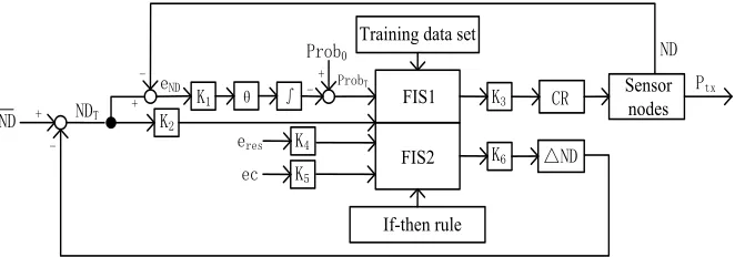
With respect to the power saving and reliability of the wireless sensor networks, it seems an impertinent approach to only apply a single fuzzy logic system when adjust-ing transmission power. Therefore, a neural fuzzy controller based system which consists of two inference engines is designed to adaptively adjust the transmission power according to the residual energy of the node with desired node degree. By means of applying the self-learning neural network, the first inference engine (FIS1) can learn from training data set to control transmission power. And by using the rules from domain experts, the second inference engine (FIS2) can adjust the targeted node degree according the residual energy. The architecture of NDPC is illustrated in Fig.1.

FIS1

FIS2

Training data set

If-then rule

Sensor nodes

Fig. 1. Architecture of NDPC

3.1 Input and output

As seen from Fig.1, NDPC consists of two inference engines which have a

com-mon input denoted by desired node degree ND. Also ND is used to calculate the

targeted node degree NDT by adding the variation to be applied !ND estimated by

FIS2 based on the residual energy. In addition, the other input of FIS1 is the

probabil-ity Prob that a node has degreeND. Moreover, adjusting the transmission power is a

very common capability in many sensor nodes, hence, the output of FIS1 is the

second input of FIS2 is the residual energy deviation

e

res_{, the third input is the ratio} of residual energy and the deviation of communication range, that is

ec e e

=

res

/

cr_. K1

!K2!K3!K4!K5and K6 in Fig.1 are scale factors.

The probability that the node degree is at least bigger than

k

is given by Eq.(1) as

in [22].

2

2 1

0

(

)

(

)

( , ) 1

!

N k

r

N

r

P ND k

f k r

e

N

!"

!"

#

#

=

$

=

=

#

%

(1)

where

r

is the node communication radius,

n

A

!

=

is node density,

n

is the total

number of nodes in the network, and

A

is the area of the field of interest. As

illustrat-ed in Fig.1 and Eq.(1), the inputs of FIS1 are _ND and Prob, and the output is

P

_tx.

Given the above parameter values, CR {r ,r ,...,r }! 1 2 j ,and ND {k ,k ,...,k }! 1 2 m ,

then Prob= f ND CR( , ) can be calculated from Eq. (1). The training data set

T

is

a s!3matrix in the form of [ND Prob CR, , ], where

s m j

=

!

.

For the energy model, the first order radio model described in [22] is adopted to

calculate the residual energy deviation. For the pair of nodes

i j

,

, the energy

con-sumed in the transmit state with

l

-byte and receive state with

m

-byte for a linear

communication as a function of the distance

d

_ij is given by Eq. (2).

4

8 (

)

I e r ij e

E E

lE lE d

mE

!

=

" #

+

+

(2)

Where

E

_Iis the residual energy before the transmission, and _Eeis the energy

con-sumed by the corresponding electronic circuits, and

E

_r is the energy consumed by

the power amplifier. Like in [22], the parameters of

E

_e,

E

_rare both assumed to be

50 /nj bit.

3.2 The first inference engine

input layer input variable membership function layer rule layer output layer adaptive computing layer

Fig. 2. Architecture of FIS1

(1) Input layer: The network has two inputs, namely ND and Prob!

(2) Membership functions layer: According to the collected data of ND ,Prob

and CR, the training data set [ND Prob CR, , ]is obtained which is used for training

the model. For the

j

_th data set, the bell-shaped function is used to fuzzy the input

variables. Membership function of each variable is given by Eq. (3).

2 2

(

) exp(-(

- ) / ) ( 1,2)

(

) exp(-(

- ) / )

j _{i i}

i _{j j}

j i i

i j j

PRR

PRR c

b

i

Prob

Prob c

b

µ

µ

!"

=

=

#

=

"$

(3)

Where

i

is the number of fuzzy subsets, and i

,

i

j j

c b

are the center and width of

membership functions.

(3) Rule layer: The fuzzy operation is performed on the data. And the output is the normalized value of each neuron input product, namely the normalization of the exci-tation intensity of each rule, which is shown as follows:

T T

ND _a Prob_b

j

R

=

µ

!

µ

4)

1 2 j j mn

R

R

R R

R

=

+

+

!

+

5)

Where Rj means rule

j

, a!

{

1,2, ,! m

}

, b!

{

1,2, ,! n

}

, j=1,2,3, ,! mn.

T T

(

ND

j

Prob

j

)

j j j j j j j

C

=

R f

=

R p

!

+

q

!

+

r

(6)

Where

{

p q rj, ,j j

}

are the node's parameters.

(5) Output layer: The total network training output represents the node communi-cation range value, which is predicted from the expected energy consumption and packet size of the input node, and the result is the sum of the four outputs in the adap-tive computation layer:

1 2 3

CR

=

C C C

+

+

+

!

+

C

mn (7)

(6) Learning process: given the learning error function as follows:

2

1 (CR CR )

2

d c

e

=

!

(8)

Where CRd,CRcare the desired and real communication range of the node. Then

the system adjusts the parameters weight vale

!

, the center and width values

c b

of

the membership function to achieve the desired effect by continuous learning. And the parameters can be obtained by Eq. (8) (9) (10) respectively.

( )

k

(

k

1)

e

!

!

"

!

#

=

$ $

#

(9)

( ) ( 1) e

c k c k

c

!

" = # #

" (10)

( ) ( 1) e

b k b k

b

!

" = # #

" (11)

Where

k

is the number of learning process, and

!

is the learning rate.

3.3 The second inference engine

FIS2 uses Mamdani-type fuzzy controller to adaptively adjust the desired node degree through the closed-loop feedback mechanism to obtain the optimal target node

degree. The input variables of FIS2 are the ratio of the target node degree NDT, the

remaining energy deviation eres and the ratio ec=eres/ecr of the remaining energy deviation and the communication range deviation, and the output variable is the

ex-pected node deviation !ND. FIS2 mainly consists of several parts like fuzzification,

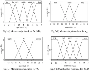
fuzzy rule, and defuzzification which are described in detail next. (1) Fuzzification

The clear value of the target node degree NDT of the input variable is [0, 1, 2, 3,

devi-ation eres of the input variables is [0, 1, 2], and the corresponding fuzzy language vari-ables are "small", "middle" and "large"; and the clear value of the ratio ec of the remaining energy deviation and the communication range deviation is [-1, 0, 1], and the corresponding fuzzy language variables are "negative", "O" and "positive"; the

clear variable of desired node degree deviation !ND of the output variable is [2,

-1,0,1,2], and its corresponding fuzzy language variables are "D2S", "D1S", "HOLD", "U1S", "U2S ". Besides, "low", "high", "small", "large", "negative", "positive", "D2S" and "U2S" are the trapezoidal membership functions, while "low_middle", "middle", "middle_high", " O "," D1S "," HOLD ", and" U1S "are triangular membership func-tions. Input and output variables membership functions are shown in Fig.3.

0 2 4

0 0.5

1 low low_middle middle middle_high high

input variable

0.5 1 1.5 2.5 3 3.5

m

em

be

rs

hi

p

0 1 2

0 0.5

1 small middle large

input variable

0.2 0.4 0.8 1.2 1.4 1.8

me

mb

er

sh

ip

0.6 1.6

Fig.3(a) Membership functions for NDT Fig.3(b) Membership functions for eres

-1 0 1

0 0.5

1 negative O positive

input variable

-0.8 -0.6 -0.2 0.2 0.4 0.8

me

mb

er

sh

ip

-0.4 0.6

-2 0 2

0 0.5

1 D2S D1S HOLD U1S U2S

output variable

-1.5 -1 -0.5 0.5 1 1.5

me

mb

er

sh

ip

Fig.3(c) Membership functions for

ec

Fig.3(d) Membership functions for !ND

Fig. 3. Membership functions for inputs and outputs

Fuzzy rules and defuzzification. Using the membership functions given above,

Table 1. Fuzzy rules

No. Input Output

T

ND

e

_res ec !ND

1 low small negative HOLD

2 low small O HOLD

3 low small positive D1S 4 low middle negative D1S

5 low middle O D1S

6 low middle positive D2S 7 low large negative D1S

8 low large O D2S

9 low large positive D2S 10 low_middle small negative HOLD 11 low_middle small O D1S 12 low_middle small positive D2S 13 low_middle middle negative HOLD 14 low_middle middle O D1S 15 low_middle middle positive D1S 16 low_middle large negative HOLD 17 low_middle large O HOLD 18 low_middle large positive D1S 19 middle small negative HOLD

20 middle small O HOLD

21 middle small positive HOLD 22 middle middle negative U1S

23 middle middle O HOLD

24 middle middle positive HOLD 25 middle large negative U1S

26 middle large O U1S

27 middle large positive HOLD 28 middle_high small negative U1S 29 middle_high small O HOLD 30 middle_high small positive HOLD 31 middle_high middle negative U2S 32 middle_high middle O U1S 33 middle_high middle positive U1S 34 middle_high large negative U2S 35 middle_high large O U2S 36 middle_high large positive U1S 37 high small negative U1S

38 high small O HOLD

40 high middle negative U2S

41 high middle O U1S

42 high middle positive U1S 43 high large negative U2S

44 high large O U2S

45 high large positive U1S

Then, the centroid method is adopted to defuzzify the output in order to get the clear output value, which is given by Eq. (12).

!ND 1

!ND 1

( ) !ND

( ) n

i i

i n

i i

x x

x

µ

µ

=

=

=

!

!

(12)

3.4 NDPC algorithm

The fuzzy neural controller designed above can be constructed with ANFIS, an adaptive fuzzy neural system tool in MATLAB, besides, evalfis is a function of the fuzzy inference system in MATLAB, representing FIS1 of NDPC. FIS2 is represented by

fis2(ND , , )

_T

e ec

. A node in the network initially broadcasts a HELLO message in

the maximum communication range rmax, which contains its unique id, to collect its

neighbor information and obtain its actual node degree and remaining energy value. Then the data can be written into the fuzzy neural controller to adaptively control the communication range. The algorithm pseudo code is shown as follows.

It is given that:

1: training set: T=[ND ,Prob ,CR]T T ;

2: the maximum communication range of the node: rmax;

3: the expected node degree: _ND, the deviation of the node degree: eND; the

threshold of the node deviation: e_ND; 4: initial energy: Einit;

5: the number of cycles:

rounds

=0;

6:

!

0=0.02�Prob0=0.8;

The algorithm starts:

7: Obtain the fuzzy neural controller by ANFIS(T); 8: CRu!rmax;

9:

e

_res

(rounds)

= E

_init; 10: do�

11: Broadcast HELLO message with current CRu

12: For messages received from other nodes, store the ID of its neighbors;

ener-14: computing the target node degree: ND =ND-!NDT and the deviation of the node degree eND=ND -NDT ;

15: rounds+ =1; computing the remaining energy deviation

res(rounds) res(rounds+1)

e e= !e ;

16: if eND>0 then

17: 0

2

!

! = ;

18: else 19: ! != 0;

20: end if

21: ProbT"Prob0#

%

!$eND;

22: fis2(ND , ,ec)Te ;

23: CRu!evalfis(ND ,Prob )T T ; 24: while(eND>eND);

25: end;

4

Simulation results

In order to verify the performance of NDPC algorithm, ATPC[5], FCTP[12], FTC[22] and NDPC are compared towards the average energy consumption, packet rate and network lifetime under MATLAB simulation environment. MICA2 is chosen as the simulation node. It is given that all nodes are randomly distributed in an area of

200m 200m! _{, the coordinates of the sink node are} (100,100)_{, the initial energy of}

nodes is 1J, the number of transmission data bits is 4000bits, the packet size is 500bytes and the control packet size is 25bytes. Besides, the scale factors are based on the real parameters of MICA2. Set K1=6, K2=2, K3=5,

K

4

=

0.5

_, K5=4,

6 3

K = _{. The simulation results are the average of 50 experimental results.}

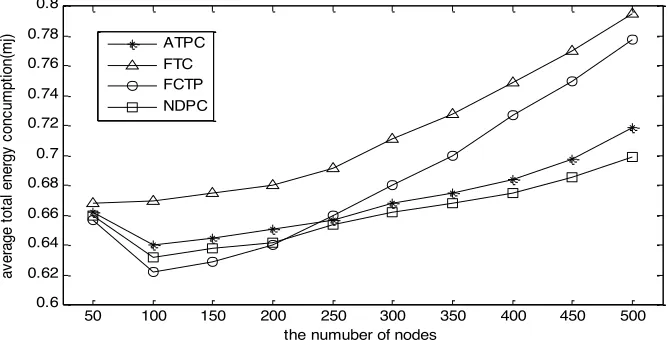
Firstly, the relationship in the algorithm between the nodes’ average total energy consumption and the network capacity is tested. The average total energy consump-tion of the nodes is the average of the total energy consumpconsump-tion of all the nodes in the network. The result is shown in Fig.4.

Fig. 4. Average total energy consumption of the nodes versus the number of nodes

pared with FCTP, NDPC uses two fuzzy inference systems in the adjustment pro-cess.Although the adjustment value of the adjusted transmission power is better, the calculation is slightly larger than FCTP. When the number of nodes is small, the aver-age total energy consumption of NDPC is less than that of FCTP. With the expansion of network size, FCTP has too many premature death nodes and the overall perfor-mance declines. NDPC considers the remaining energy of the node to adjust its transmitting power, resulting in more balanced energy consumption. ATPC adjusts the transmit power of nodes according to the feedback of link quality to maintain high packet rate. Compared with FTC, FCTP and NDPC, ATPC can adjust faster and can reduce the average total network energy consumption. However, maintaining a high packet-receiving rate also requires a larger transmitting power. Without consideration of the remaining energy, in order to maintain a high packet-rate, nodes with a low residual energy will die early because of using a larger power transmission. In the adjustment of the transmitting power, NDPC not only adjusts the step size but also considers the residual energy of the node, thus effectively improving the network energy utilization efficiency.

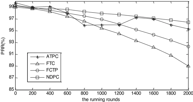
Next, the network packet rate (PRR) has been tested with 300 nodes. The result of the test is shown in Fig.5. As can be seen from the figure, since the FTC only consid-ers the target node degree of the node and ignores the link quality, the reliability of the link between the nodes and the PRR both decreases rapidly with the increase of the number of running cycles. However, FCTP takes the adjustment of the step length into account and adopts a non-linear method to adjust the transmit power of nodes. This method has a fast convergence, and it is easy to maintain the corresponding link quality. So the decrease of PRR is slower than that of FTC. The ATPC algorithm mainly considers the link quality in the process of adjusting the transmit power, and its feedback regulation goal is to maintain a certain packet reception rate, so the PRR can be hold at a high level. However, as the number of running rounds increasing, the

50 100 150 200 250 300 350 400 450 500

0.6 0.62 0.64 0.66 0.68 0.7 0.72 0.74 0.76 0.78 0.8

av

er

age t

ot

al ener

gy

c

onc

um

pt

ion(

m

j)

the numuber of nodes ATPC

ers not only the residual energy of nodes but also the adjustment of step size. It does improve the robustness. Therefore, the PRP of NDPC can stay at a high and steady state.

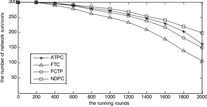
Finally, the network life cycle has been tested based on the survival nodes with 300 nodes. The result is shown in Fig.6. Because the other three algorithms do not consid-er the remaining enconsid-ergy of nodes, it is easy to cause nodes with low remaining enconsid-ergy dying early at a high transmit power. FTC adjusts the transmission power through the learning of the data, it is not easy to obtain the optimal transmission power, and the adjustment is more frequent, which leads to a waste of the most energy. FCTP adjusts the adjustment step size according to the degree of node deviation, reducing the num-ber of adjustment, which reduces the energy consumption compared with FTC. How-ever, the APTC adjusts the transmit power by means of link quality feedback, so that it can be quickly adjusted to meet a certain packet receiving rate. This method has a faster adjustment speed and lower communication energy consumption. However, NDPC can adjust its transmission power through data learning, it adaptively change the step size to accelerate the convergence. Considering the remaining energy of the node, NDPC avoids nodes with low remaining energy from transmitting data with high power, thus prolonging the network life cycle.

Fig. 5. Average PRR versus the running rounds

0 200 400 600 800 1000 1200 1400 1600 1800 2000

85 87 89 91 93 95 97 99

PRR(

%

)

the running rounds ATPC

Fig. 6. The number of network survivors versus the running rounds

5

Conclusion

In this paper, a power control method based on fuzzy neural controller (NDPC) has been proposed. It consists of two fuzzy inference systems, and it adaptively adjusts the target node degree according to the residual energy of nodes to control the node transmission power. The simulation results show that NDPC has a better performance in terms of total node average energy consumption, packet rate and network life cycle than APTC, FTC and FCTP, which can effectively reduce node energy consumption and extend network life cycle.

6

Acknowledgment

This work was supported by Jilin Provincial Development and Reform Commis-sion Project (2018C039-2); Science and technology program of Jilin provincial sci-ence and Technology Department (20150204073GX); Jilin Provincial Department of science and technology pilot project (20160312002ZG).

7

References

[1]TAHAR E, AMIRA Z. Efficient measurement of temperature, humidity and strain varia-tion by modeling reflecvaria-tion Bragg grating spectrum in WSN[J]. Optik - Internavaria-tional Jour-nal for Light and Electron Optics, 2017, 135:454-462!

[2]JAVIER L, RUBEN R, FENG B, et al. Evolving privacy: From sensors to the Internet of Things[J]. Future Generation Computer Systems, 2017, 75: 46-57!https://doi.org/10.1016/j.future.2017.04.045

0 200 400 600 800 1000 1200 1400 1600 1800 2000

50 100 150 200 250 300

the num

ber

of

net

wor

k s

ur

vi

vor

s

the running rounds ATPC

[3]Xue Z. Topology Control for Wireless Sensor Networks[J]. Journal of Software, 2007, 18(4): 943-954. https://doi.org/10.1360/jos180943

[4]PANTAZIS N A, VERGADOS D. A survey on power control issues in wireless sensor networks[J]. IEEE Communications Surveys & Tutorials. 2007, 9(4): 86-107!https://doi.org/10.1109/COMST.2007.4444752

[5]SHAN L, FEI M, ZHANG J B, et al. ATPC: Adaptive Transmission Power Control for Wireless Sensor Networks[J]. ACM Transactions on Sensor Networks, 2016, 12(1):6! [6]HUSEYIN U Y, BULENT T. Transmission power control for link-level handshaking in

wireless sensor networks[J]. IEEE Sensors Journal. 2016, 16(2): 561-576!https://doi.org/10.1109/JSEN.2015.2486960

[7]HUSEYIN C, KEMAL B, BULENT T, et al. The impact of transmission power control strategies on lifetime of wireless sensor networks[J]. IEEE Transactions on Computers. 2014, 63(11): 2866-2879. https://doi.org/10.1109/TC.2013.151

[8]Son B H, Kim K J, Choi Y M. Active-margin transmission power control for wireless sen-sor networks. International Journal of Distributed Sensen-sor Networks. 2014, 2014(1): 1-7. [9]LIU T. Distributed power control mechanism based on utility model in wireless sensor

networks [J]. electronic journal, 2016, 44(02): 301-307.

[10]GUO Z Q, WANG Q, LI M H, et al. Fuzzy Logic Based Multidimensional Link Quality Estimation for Multi-Hop Wireless Sensor Networks[J]. IEEE Sensors Journal, 2013, 13(10):3605-3615!https://doi.org/10.1109/JSEN.2013.2272054

[11]KUUBISCH M, KARL H, WOLISZ A, et al. Distributed algorithm for transmission power control in wireless sensor networks[C]. Wireless Communications and Networking, WCNC 2003. USA, New Orleans, IEEE, 2003(1): 558-563.

[12]Zhang J, Chen J, Sun Y. Transmission power adjustment of wireless sensor networks using fuzzy control algorithm[J]. Wireless Communications & Mobile Computing, 2009, 9(6):805-818. https://doi.org/10.1002/wcm.630

[13]VICENTE H D, JOSE F M, NESTOR L M, et al. Self-adaptive strategy based on fuzzy control systems for improving performance in wireless sensors networks[J]. ACM Trans-action on Sensor Networks. 2015, 15(9): 24125-24142!

[14]NARAYANASWAMY S, KAWADIA V, and SREENIVAS R S, et al. Power control in Ad-Hoc networks: theory, architectur, algorithm and implementation of the COMPOW protocol[C]. In Proceedings of the European Wireless Conference. 2002, PP: 156-162. [15]SANTI P, BLOUGH D M, BOSTELMANN H. The critical transmitting range for

connec-tivity in sparse wireless ad-hoc networks[J]. IEEE Transactions on Mobile Compu-ting.2003, 2(1): 25-39!https://doi.org/10.1109/TMC.2003.1195149

[16]Lim G. Link Stability and Route Lifetime in Ad-hoc Wireless Networks[C]. IEEE Parallel Processing Workshops International Conference, 2002:116-123.

[17]Senouci M R, Mellouk A, Senouci H, et al. Performance evaluation of network lifetime spatial-temporal distribution for WSN routing protocols[J]. Journal of Network & Com-puter Applications, 2012, 35(4):1317-1328. https://doi.org/10.1016/j.jnca.2012.01.016

[18]Yanagihara K, Taketsugu J, Fukui K, et al. A Clustering Scheme with Transmission Power Control for Sensor Networks[J]. Ieice Technical Report, 2005.

[19]Wang J, Yang L S, Zhao Y F. Research of Forestry Monitor Wireless Sensor Networks Cross-layer Power Control Based on Link Quality[J]. Radio Communications Technology, 2010.

[20]Sun Hongliang, Lu Hongbin. Measurement and Analysis of Environmental Impact on Wireless Link Quality[J]. China Science and Technology Expo, 2009(14):198-198. [21]MIRJANA M, VALDIMIR V, VLADIMIR M. Fuzzy Logic and Wireless Sensor

[22]HUANG Y, DIAZ VH, SENDRA J. A novel topology control approach to maintain the node degree in dynamic wireless sensor networks [J]. Sensors. 2014, 14(3): 4672-4688!https://doi.org/10.3390/s140304672

[23]Soni V, Mallick D K. Fuzzy logic based multi-hop topology control routing protocol in wireless sensor networks[J]. Microsystem Technologies, 2018(7):1-13.

8

Authors

Huangshui Hu is an associate professor in Changchun University of Technology.

He received his B.Sc. degree in 1997 from Jilin University, received his M.Sc. degree in 2005 from Jilin University, and received his Ph.D. degree in 2012 from Jilin Uni-versity. His main research interests include wireless sensor networks and train com-munication networks.

Man Zheng is a graduate student in College of Computer Science and

Engineer-ing, Changchun University of Technology. She has received her B.Sc. degree in

2016(year) from Hubei University of Arts and Science. Her main research interests include wireless sensor networks and train communication networks.

Bangcheng Zhang is a professor in Changchun University of Technology. He

re-ceived his B.Sc. degree in 1995, M.Sc. degree in 2004, Ph.D. degree in 2011 from Jilin University. His main research interests include mechatronics, complex system fault diagnosis and forecast and service robot.

Jinhui Qing is a graduate student in College of Computer Science and

Engineer-ing, Changchun University of Technology. He has received her B.Sc. degree in

2017(year) from Changchun University of Technology. His main research interests include wireless sensor networks and train communication networks.