TECHNIQUES TO EXPLOIT INSTRUCTION LEVEL PARALLELISM (ILP): A REVIEW SURVEY

(1)

Available Online at www.ijpret.com

380

INTERNATIONAL JOURNAL OF PURE AND

APPLIED RESEARCH IN ENGINEERING AND

TECHNOLOGY

A PATH FOR HORIZING YOUR INNOVATIVE WORK

TECHNIQUES TO EXPLOIT INSTRUCTION LEVEL PARALLELISM (ILP): A REVIEW

SURVEY

PROF. PRAJAKTA PANDE1, PROF. ANAND R. PADWALKAR1, MS. VIDHI DAVE2

1. Assistant Professor, Department of Computer Application, RCOEM, Nagpur. 2. TGP College of Engineering and Technology, Mohgaon, Nagpur.

Accepted Date: 27/02/2014 ; Published Date: 01/05/2014

\

Abstract: Every application, scalar or parallel, experiences a critical-path in the system capital it accesses. For a developer a basic objective is to arrange algorithms and coding techniques which reduce the total application execution time. This paper is a survey on techniques that exploit Instruction Level Parallelism (ILP). There are some machine architectures which strongly support Instruction Level Parallelism. These machines are discussed in this paper. Also the types of dependency amongst instructions are analyzed and ways in which these dependencies can be resolved to exploit Instruction Level Parallelism are studied. Compiler plays a very important role in exploitation of Instruction Level Parallelism. All the techniques used by the compiler for exploitation of Instruction Level Parallelism are examined. Added to, Pipelining can extend beyond the execution of instructions when they are independent of one another. This potential overlie among instructions is called instruction-level parallelism (ILP) since the instructions can be evaluated in parallel. The amount of parallelism available within a basic block is quite small. Since the instructions are likely to depend upon one another, the amount of overlap we can exploit within a basic block is likely to be much less than 7. To obtain substantial performance enhancements, we must exploit ILP across multiple basic blocks. The simplest and most common way to increase the amount of parallelism available among instructions is to exploit parallelism among iterations of a loop

Keywords: Recommendation, aggregation, utility matrix

Corresponding Author: PROF. PRAJAKTA PANDE

Access Online On:

www.ijpret.com

How to Cite This Article:

Prajakta Pande, IJPRET, 2014; Volume 2 (9): 380-395

(2)

381

INTRODUCTION

One of the measures of performance of a processor is Cycles per Instruction (CPI) [1]. A pipelined processor aims to CPI equal to one. i.e., to issue and retire one instruction per cycle, and it cannot achieve a lower value than this. In order to break this threshold of a CPI = 1 , two routines are followed :

 Increase the throughput through fragmentation of pipeline stages.

 Increase the number of instruction issued per cycle through presence of multiple data paths.

The first technique is called super pipelining [2]. It attempts achievement of higher performance by dividing each main pipeline stage in sub stages.

The second technique is implemented by ILP machines. To achieve a CPI less than 1 these machines issue multiple instructions per cycle into different data paths.

The first approach refers to parallelism that machine can actually exploit i. e. number of parallel data path present in the architecture. Instruction parallelism on the other hand refers to amount of parallelism found in application program. It is the maximum number of instructions that can be simultaneously executed in pipelining. In this paper we first introduce machine parallelism in different architecture philosophies, and then analyze different technique the compiler use to expose instruction parallelism in machines. An overview of architecture aspects related to ILP exploitation is introduced also a few ILP machines are discussed. The rest of the paper deals with limitations imposed on ILP by dependency among instructions and methods to deal with them.

Exploitation of Instruction level parallelism using Hardware architecture.

The traditional machines before introduction of pipelining were sequential machines. In these machines all the instructions were executed sequentially i.e. one after another. The program consists of sequence of instructions and the next instruction could be executed only after the execution of previous instruction is complete and results are written back to memory. Such type of machines had no scope for exploitation of ILP.

(3)

382

with the introduction of pipeline machines and so was the amount of parallelism the compiler must provide to keep all the hardware units busy. After this multiple issue processors [2][4] were introduced, which increased the amount of parallelism a machine can exploit. Such processors have multiple data paths for instruction execution each of them being able to issue, execute and retire one instruction per cycle.

The aim of multiple issue architecture is to exploit parallelism in application program. The instructions in program are analyzed first for data and control dependencies in order to find group of independent instructions that can be concurrently issued without altering correctness of the program. Depending on when this scheduling is performed two different approaches have been taken static and dynamic scheduling leading respectively to VLIW and Superscalar machines.

Superscalar Machines

Superscalar machines were originally developed as an alternative to vector machines. A superscalar machine of degree n can issue n instructions per cycle. For example a super-scalar machine could issue all three parallel instructions in the same cycle.

Load C1<-23(R2)

Add R3<-R3+1

FPAdd C4<-C4+C3

Super-scalar execution of instructions is illustrated in Figure below [7].

(4)

383

VLIW Machines

VLIW [7], or very long instruction word, machines typically have instructions hundreds of bits long. Each instruction can specify many operations, so each instruction exploits instruction-level parallelism. Many performance studies have been performed on VLIW machines the execution of instructions by an ideal VLIW machine is shown in Figure.

Each instruction specifies multiple operations, and this is denoted in the Figure by having multiple crosshatched execution stages in parallel for each instruction.

In VLIW case, all dependencies are checked during compile time, and the search of independent instructions and scheduling is done entirely by the compiler. All the independent instructions are grouped together and a single very large instruction word is formed to execute such operations simultaneously.

Dependency Analysis

Dependence analysis is the first step a compiler carries out in order to expose parallelism.

Two operations A and B can execute simultaneously if they are independent, that is if the two possible relative orders of execution of the two (A before B or B before A) produce exactly the same results in the overall program behavior, for every possible input data. The previous statement explains the concept of independence by giving its effect on the program. However it becomes crucial to understand what causes operations to be independent, so that independence can be detected and consequently exploited by the compilers.

(5)

384

Control Dependency

Control dependency arises when a jump instruction is encountered. They make the flow of program non sequential. The techniques to overcome control dependency are branch prediction & speculative execution .

Branch prediction and speculative execution

In the scheme we used [5, 6], the branch predictor maintains a table of two-bit entries. Low-order bits of a branch’s address provide the index into this table. Taking a branch causes us to increment its table entry; not taking it causes us to decrement. We predict that a branch will be taken if its table entry is 2 or 3. This two-bit prediction scheme mispredicts a typical loop only once, when it is exited. A good initial value for table entries is 2, just barely predicting that each branch will be taken.

Branch prediction is often used to keep a pipeline full: we fetch and decode instructions after a branch while we are executing the branch and the instructions before it. To use branch prediction to increase parallel execution, we must be able to execute instructions across an unknown branch speculatively. This may involve maintaining shadow registers, whose values are not committed until we are sure we have correctly predicted the branch. It may involve being selective about the instructions we choose: we may not be willing to execute memory stores speculatively, for example. Some of this may be put partly under compiler control by designing an instruction set with explicitly squash able instructions. Each squash able instruction would be tied explicitly to a condition evaluated in another instruction, and would be squashed by the hardware if the condition turns out to be false. Rather than try to predict the destinations of branches, we might speculatively execute instructions along both possible paths, squashing the wrong path when we know which it is. Some of our parallelism capability is guaranteed to be wasted, but we will never miss out by taking the wrong path.

True Data Dependency and Value Prediction

True data dependency occurs when value produced by an instruction is required by a subsequent instruction. It is also known as a flow dependency because dependency is due to flow of data in program and also called read-after-write hazard because reading a value after writing to it.

Example

1. ADD R3,R2,R1 ;

(6)

385

“Data” dependency between instruction 1 and 2 (R3).

In general, they are the most troublesome to resolve in hardware.

Value Prediction

Value prediction is a predictive technique used to overcome true data dependency. This technique is used to predict the value of a not yet produced operand by looking at its past history.

There are different types of architectures for value prediction. They can be classified as stride value prediction, context value prediction and hybrid value prediction.

Stride

A stride predictor keeps track of not only the last value brought in by an instruction, but also the difference between that value and the previous value. These differences called the stride. The predictor speculates that the new value seen by the instruction will be the sum of the last value seen and the stride

Context

A context predictor bases its prediction on the last several values seen. We chose to look at the last 4 values seen by an instruction. A table called the VHT( value history table)contains the last 4 values seen for each entry. Another cache, called the VPT(value prediction table), contains the actual values to be predicted. An instruction’s PC is used to index into the VHT, which holds the past history of the instruction. The 4 history values in this entry are combined (or folded) using an xor hash into a single index into the VPT. This entry in the VPT contains the value to be predicted. The context predictor is able to keep track of a finite number of reference patterns that are not necessarily constrained by a fixed stride.

Hybrid

(7)

386

False data dependency and Register Renaming

WAR write after read and WAW write after write cause false dependences. They arise only after register allocation since they are caused by the fact that physical storing location is used by two different instructions to write or read two different values.

Register Renaming

As long as free register are available, the compiler can solve a false dependence by changing the name of the register which causes the conflict.

The instruction that writes into such register is modified so that the generated value is stored in new register which is free from conflict.

By eliminating related precedence requirements in the execution sequence of the instructions, renaming increases the average number of instructions that are available for parallel execution per cycle. This results in increased IPC (number of instructions executed per cycle).

The identification and exploration of the design space of register-renaming lead to a comprehensive understanding of this intricate technique.

The principle of register renaming is straightforward. If the processor encounters an instruction that addresses a destination register, it temporarily writes the instruction’s result into a dynamically allocated rename buffer rather than into the specified destination register.

For instance, in the case of the following WAR dependency:

i1: add …., r2, …..; (…..<-(r2) + (….)]

i2: mul r2, …., ….; [r2<-. (..) *(…)]

the destination register of i2 (r2) is renamed, say to r33. Then, instruction i2 becomes

i2′ : mul r33, …., ….; [r33 …(…) * (…)]

Its result is written into r33 instead of into r2.This resolves the previous WAR dependency between i1 and i2. In subsequent instructions, however, references to source registers must be redirected to the rename buffers allocated to them as long as this renaming remains valid. [8]

COMPILER TECHNIQUES FOR EXPLOITATION OF INSTRUCTION LEVEL PARALLELISM

(8)

387

Local Techniques

Loop Dependency & Loop Transformations

Every statement can be executed multiple times within the loop and therefore dependences between statements in the same loop body but in two different iterations might arise.

These are called loop dependences.

Loop Transformation

Loop transformation is a technique which helps the scheduler to overlap successive loop iterations in an attempt to increase ILP.

Loop Peeling

Loop peeling attempts to expose more parallelism inside an inner loop. It is the process of taking off a number of iterations from a loop body and consequently express them at the beginning or end of loop.

For Example:

for(i=0;i<102;i++)

A[i]=A[i-1]+c;

for(i=0;i<100;i++)

A[i]=A[i-1]+c;

A[100]=A[99]+c;

A[101]=A[100]+c;

As shown in the example above a loop that was iterated 102 times is transformed in consequence to application of loop peeling into a loop iterated 100 times and followed by the last two iterations explicitly expressed. This is often done in order to match two different bounds of two subsequent loops. This technique is useful when used in conjunction with loop fusion.

Loop Fusion

(9)

388

Loop Fusion is often applied in combination with peeling, when two loops follow each other sequentially, but they have slightly different bounds. Peeling is first applied: iterations exceeding the bounds are 'peeled of' from the 'uneven' loop, so that bounds become balanced.

Example in C

for (i = 0; i < 102; i++)

a[i] = a[i-2]+5;

for (j = 0; j < 100; j++)

b[i] =b[i]* 2;

is equivalent to:

for (i = 0; i < 100; i++)

{ a[i] = a[i-2]+5;

b[i] = b[i]*2; }

a[100]=a[98]+5;

a[101]=a[99]+5;

After peeling, the two bounds are identical and the loops can be fused. This means that instructions from both loop bodies are fused together so that only one loop body results.

Instructions inside each original loop can now be parallelized, as shown in example. Loop fusion exposes more parallelism if instructions from the original bodies are independent of each others, so that they can be parallelized after fusion.

Loop Unrolling

(10)

389

Example

A procedure in a computer program is to delete 100 items from a collection. This is normally accomplished by means of a for-loop which calls the function delete(item_number). If this part of the program is to be optimized, and the overhead of the loop requires significant resources compared to those for the delete(x) loop, unwinding can be used to speed it up.

Normal loop After loop unrolling

int x;

for (x = 0; x < 100; x++)

{

delete(x);

}

int x;

for (x = 0; x < 100; x+=5)

{delete(x); delete(x+1);

delete(x+2);

delete(x+3);

delete(x+4);

}

As a result of this modification, the new program has to make only 20 iterations, instead of 100. Afterwards, only 20% of the jumps and conditional branches need to be taken, and represents, over many iterations, a potentially significant decrease in the loop administration overhead. Also copying the body of the loop a number n of times, and then iterating with step n (where the induction variable is now increased by five every iteration, after unrolling of a factor of five). The loop body results n times longer and, as a result of it, there is a higher number of candidates for parallel execution.

Loop fission

Loop fission (or loop distribution) is a compiler optimization in which a loop is broken into multiple loops over the same index range with each taking only a part of the original loop's body. The goal is to break down a large loop body into smaller ones to achieve better utilization of locality of reference. This optimization is most efficient in multi-core processors that can split a task into multiple tasks for each processor. It is the opposite to loop fusion, which can also improve performance in other situations.

Example in C

(11)

390

for (i = 0; i < 100; i++)

{

b[i]=b[i-1]+c;

a[i]=b[i]+2;

}

is equivalent to

int i, a[100], b[100];

for (i = 0; i < 100; i++) {

b[i]=b[i-1]+c;

}

for (i = 0; i < 100; i++) {

a[i]=b[i]+2;

}

An example of code where loop distribution is useful is shown above. Instructions in the original loop cannot be parallelized because the second instruction depends on the first one.

On the other hand, there is no need to execute them in the same loop (the first instruction does not depend on previous iterations of the second one), and the loop can be distributed into the two subsequent sub-loops shown above. And therefore parallelism can be used.

Software Pipelining

Software pipelining parallelizes loops by starting a following iteration before the previous ones have terminated execution. This is where analogy from the hardware pipeline counterpart comes from.

Consider the following loop:

for (i = 1) to big number

A(i)

B(i)

C(i)

(12)

391

In this example, let A(i), B(i), C(i), be instructions, each operating on data i, that are dependent on each other. In other words, A(i) must complete before B(i) can start. For example, A could load data from memory into a register, B could perform some arithmetic operation on the data, and C could store the data back into memory. However, let there be no dependence between operations for different values of i. In other words, A(2) can begin before A(1) finishes.

Without software pipelining, the operations execute in the following sequence:

A(1) B(1) C(1) A(2) B(2) C(2) A(3) B(3) C(3) ...

Assume that each instruction takes 3 clock cycles to complete (ignore for the moment the cost of the looping control flow). Also assume (as is the case on most modern systems) that an instruction can be dispatched every cycle, as long as it has no dependencies on an instruction that is already executing. In the unpipelined case, each iteration thus takes 7 cycles to complete (3 + 3 + 1, because A(i+1) does not have to wait for C(i))

Now consider the following sequence of instructions (with software pipelining):

A(1) A(2) A(3) B(1) B(2) B(3) C(1) C(2) C(3) ...

It can be easily verified that an instruction can be dispatched each cycle, which means that the same 3 iterations can be executed in a total of 9 cycles, giving an average of 3 cycles per iteration.

Note that the great advantage of software pipelining over loop unrolling is that the former does not increase code length: instead of duplicating the loop body, software pipelining modifies it so that it is still composed by the same number of instructions, but these come from different iterations of the original loop.

Global Techniques:

Trace Scheduling

Trace is defined as the collection of basic blocks in a code that follows a single path. A trace may include branch but loops are not allowed to be a part of a trace. In many applications, the loops are unrolled to a degree that matches the throughput requirement with the parallel mapping possible in the shared hardware resource. Once the traces are identified in a code, the scheduling of these traces for optimal code execution is known as trace scheduling.

(13)

392

executed [13]. In other words, it is the sequence of instruction with only one entry and one exit. The basic block does not contain any control flow into or out of the basic block. Control flow in a basic block can only be found at its beginning or end. Compensation or fix-up code is required at the beginning (entrance) or end (exit) of the basic block so that the control flow may enter or exit into/out of the basic

block. The first scheduled trace of a code has to be the path which has the maximum likelihood to be executed through the program [14].

This would result in a schedule optimal for the most common flow through the program. The basic idea behind trace scheduling is to increase ILP in the most probable code flow by removing unimportant code path.

Directed acyclic graph (DAG) is a tool used for scheduling traces. The first step before scheduling is to identify the traces in a given DAG [14]. The trace which will be scheduled first will be the most probable flow through the graph. Similarly the next most probable trace will be eligible for scheduling and so on until all identified traces in a DAG are scheduled. However, if trace ‘x’ may branch into trace ‘y’, a fix up or compensation code is inserted between trace ‘x’ and trace ‘y’ so that the resource integrity associated with trace ‘y’ is justified [14]. Similarly in case if trace ‘y’ needs to branch into trace ‘x’, a compensation code is introduced between the two traces.

Trace Scheduling can be summarized as a collection of following steps:

1. Select a trace from the program.

2. Schedule the selected trace.

3. Insert the fix up/ compensation code

4. Select a new trace and repeat steps 2-3.

Superblock Scheduling

A superblock is a block of operations which has only one entry but one or more exit points.

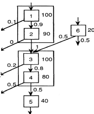
Superblocks are formed such that all operations in a superblock are likely to be executed; early exits are infrequently taken. Within a superblock, the compiler schedules operations to generate denser code by speculatively moving operations up past branches.

(14)

393

segment of a program as a control flow graph annotated with profiling information. Each basic block is annotated with its execution count. Each control flow arc is annotated with the branch probability. A possible trace is constructed as blocks 1, 2, 3 and 4 together. But a side entrance into block 3 precludes the formation of one large superblock. Instead, blocks 1 & 2 and blocks 3 & 4 are fused to form separate superblocks. Intuitively, the longer a trace the more opportunity the scheduler has to generate denser code. However, large superblocks are rare in common program graphs.

Effect of superblock scheduling

(15)

394

On the average, without applying tail duplication and loop unrolling, there are 2.49 basic blocks in a superblock; with tail duplication and loop unrolling, the average is 3.89. The average number of operations issued per cycle increased from 1.36 for ordinary blocks to 1.62 for superblocks. It should be noted that because of the speculative execution of operations inside superblocks, not all operations issued inside superblocks are useful. Nevertheless, the decrease in a schedule's length is indicative of performance improvement.

REFERENCES

1. P. G. Emma. Understanding some simple processor-performance limits. IBM Journal of Research and Development, 41(3):215{232, May 1997.

2. M.J. Flynn. Computer Architecture: Pipelined and Parallel Processor Design. Jones and Bartlett Publishers, 1995.

3. J.E. Smith and S. Weiss. PowerPC 601 and Alpha 21064: A Tale of Two RISCs. IEEE Computer, pages 46{58, June 1994.

4. J.E. Smith and G.S. Sohi. The Micro architecture of Superscalar Processors. Proceedings of the IEEE, pages 1609{1624, December 1995.

5. Johnny K. F. Lee and Alan J. Smith. Branch prediction strategies and branch target buffer design. Computer 17,pp.6-22, 1984.

6. J. E. Smith. A study of branch prediction strategies. Eighth Annual Symposium on Computer Architecture, pp. 135-148. Published as Computer Architecture News9 (3), 1986.

7. Available Instruction- Level Parallelism for Superscalar and Super pipelined Machine Norman

P. Jouppi and David W. Wall WRL Research

(16)

395

8. D. Sima, T. Fountain, and P. Kacsuk, Advanced Computer Architectures, Addison Wesley Longman, Harlow, England, 1997.

9. R.M. Tomasulo, “An Efficient Algorithm for Exploiting Multiple Arithmetic Units,” IBM J.

Research and Development, Vol. 11, No.1, 1967, pp. 25-33.

10.G.S. Tjaden and M.J. Flynn, “Detection and Parallel Execution of Independent Instructions,”IEEE Trans. Computers, Vol. C-19,No. 10, 1970, pp. 889-895.

11.R.M. Keller, “Look-Ahead Processors,” Computing Surveys, Vol. 7, No. 4, 1975, pp.177-195.

12.Joseph A. Fisher, “Trace scheduling: A technique for global microcode compaction”. IEEE Trans. Computers, 30(7): 478-490 (1981)

13.Steven S. Muchnik Advanced Compiler Design Implementation, ISBN 1-55860-320-4, Morgan Kaufmann Publishers, 1997.

14.Randy Allen, Ken Kennedy, Optimizing Compilers for modern

2. Architectures, ISBN 1-55860-286-0, Morgan Kaufmann Publishers, 2002.

15.Software Pipelining and Superblock Scheduling: Compilation Techniques for VLIW Machines Meng Lee, Partha Tirumalai, Tin-Fook Ngai Computer Systems Laboratory HPL-92-78 June, 1992

16.Kennedy, Ken; & Allen, Randy. (2001). Optimizing Compilers for Modern Architectures: A