Volume 10, Number 2, pp. 131–146. http://www.scpe.org 2009 SCPE
THE IMPACT OF WORKLOAD VARIABILITY ON LOAD BALANCING ALGORITHMS∗
MARTA BELTR ´AN† AND ANTONIO GUZM ´AN†
Abstract. The workload on a cluster system can be highly variable, increasing the difficulty of balancing the load across its nodes. The general rule is that high variability leads to wrong load balancing decisions taken with out-of-date information and difficult to correct in real-time during applications execution.
In this work the workload variability is studied from the perspective of the load balancing performance, focusing on the design of algorithms capable of dealing with this variability. In this paper an exhaustive analysis is presented to help users and administrators to understand if their load balancing mechanisms are sensitive to variability and to what degree. Furthermore, solutions to deal with variability in load balancing algorithms are proposed and their utilization is exemplified on a real load balancing algorithm.
Key words: cluster computing, load balancing, workload variability
1. Introduction. Cluster systems are rapidly evolving from laboratories and research centers to busi-ness environments due to their potential to take advantage of old and/or idle computers ([9]). In this kind of environment cluster systems are even more dynamic and variable than in the typical controlled research environments.
Many factors contribute to the system state variability ([5]): asynchronous scheduling and communication behavior arising from the autonomy of the individual system nodes (clusters are loosely-coupled systems), per-formance heterogeneity (processing nodes are rarely homogeneous, differing in many ways), workload variability (the presence of background tasks constitutes an important source of variability), variation in the number of sys-tem nodes, independent failure and recovery of nodes and variable communication latencies (network variability due to transmission errors or congestion).
Load balancing is essential to take advantage of all the available resources on cluster systems and therefore, to obtain their optimal performance ([9, 13]), especially on heterogeneous clusters. And the ability to deal with variability is essential for designing efficient and scalable load balancing algorithms. All the decisions related to load balancing are taken considering some kind of system state information. If this state suffers smooth variations, it is easy to maintain updated information about it. But when the system state is highly variable, the information may be out of date by the time the load balancing decisions are taken. Therefore, the probability of taking wrong decisions increases critically ([17]).
As far as we know the impact of workload variability on load balancing performance has not been investi-gated in detail. Some works have discussed similar problems in other research areas as networking ([1, 10, 11]), multimedia applications ([14]) or performance prediction ([12]), studying the variability of TCP round-trip times or another network aspects, execution times or processes arrivals respectively.
The main contribution of this paper is an exhaustive analysis of the effects of variability on load balancing algorithms performance. Furthermore, solutions for the main problems caused by these effects, related to the state information updating and to the load balancing operations, are presented. The proposed techniques can be used in any variable environment, typically a non-dedicated cluster, to obtain the desired performance with a load balancing algorithm. Two different robustness metrics have been proposed to select the best distribution rule for the algorithm, remote execution or process migration. With the proposed solution only when a high variability causes an intolerable performance degradation the process migration is used to balance the load in the system.
The rest of this paper is organized as follows. Section 2 studies the effects of workload variability on load balancing performance. To do this, load balancing algorithms are divided into four policies or rules. Section 3 proposes solutions to deal with variability in the information rule and discusses three different metrics to quantify the workload variability. Section 4 proposes solutions to deal with variability in the distribution rule and defines the robustness metric. Section 5 presents some experimental results to verify the performed analysis and to select a best variability metric. And finally, Section 6 summarizes conclusions and future work.
∗Questions, comments, or corrections to this document may be directed to Marta Beltr´an.
†Computer Architecture, Artificial Intelligence and Computer Science Department, Rey Juan Carlos University, Madrid, Spain
({marta.beltran, antonio.guzman}@urjc.es).
2. Effects of workload variability on load balancing. To study the effects of variability on load balancing performance, the structure of a load balancing algorithm has been decomposed in this research with the four rules or stages proposed in [19]. Another structures for the load balancing algorithm could be used to make easier the analysis of the effects of variability, but the results would be the same because it is only an structural issue and finally all the algorithms perform similar stages to balance the system load. These are the four considered rules ([8]):
• Load Measurement: Load balancing decisions always rely on some kind of workload or availability information of system nodes. This information is typically quantified by a load index in this first algorithm stage.
• Information Rule: The information policy or rule specifies how to exchange the state information between the system nodes. A good information rule should achieve a balance between incurring a low communication overhead for the state information exchange and maintaining an accurate view of the system state.
• Initiation Rule: This load balancing stage determines when to initiate a load balancing operation. These operations introduce a non-negligible overhead in the system; the initiation rule must weigh their cost against their expected performance benefit.
• Load Balancing Operation: This last rule is decomposed in three more rules: the location, distri-bution and selection rules.
The location rule determines the best candidate to participate in the load balancing operation. The distribution rule specifies how to balance the load among the nodes involved in the load balancing operation. This balance can be performed by remote execution (non-preemptive allocation or initial placement of tasks) or by process migration. And finally, the selection rule chooses the load that is going to be distributed or re-distributed with this operation.
Analyzing the effects of high workload variability on these four stages, some important conclusions can be drawn.
The effects of workload variability on the first algorithm stage depend on the selected load index. If it is a good load index, it should be able to show the workload variations summarizing the node state and maintaining its stability. Therefore, this stage performance depends entirely on the selected load index, and with the proper decision, the first algorithm stage will be able to deal with variability.
On the other hand, the impact of variability on the information policy is very important. If there is a low variability this policy has an easy job because it is not difficult to maintain updated system state information in all the cluster nodes. But if the workload variability is high, the job of this policy is more difficult because it has to maintain updated state information in all the cluster nodes without causing a great network overhead with the messages generated to do it.
For the initiation policy, all the effects of variability are related to the information rule. If this rule is capable of dealing with variability and of maintaining updated state information in all the system nodes, the initiation decisions are correct and the variability does not affect this algorithm stage.
Finally, the load balancing operation performance can be affected by the workload variability in the location and distribution rules. The location rule selects the best candidate to participate in the load balancing operation. Supposing that the system state information available to decide about this aspect is updated, there is still one problem: in a highly variable environment the system state may change during this rule. The best candidate for the load balancing operation in a certain moment may be the worst immediately after.
Considering this discussion, there are three main challenges that need to be faced: the load index selection, the information policy design and the load balancing operation execution. The load index selection is not included in this paper because it is a whole important research area in load balancing, but next sections try to propose solutions for the two other challenges.
3. Information rule capable of dealing with variability. Three different policies have been tradition-ally proposed for the information rule in load balancing algorithms:
• Periodic (or batch) policy: Each system node periodically broadcasts its state information through the system, regardless of whether this information is needed or not. In this kind of policy a critical question is to fix the interval between successive information exchanges, the information period (Tinf o).
• On-demand policy: Each system node sends a request message to the rest of the system nodes when it needs the information to make a load balancing decision.
• Event-driven policy: The information exchange is asynchronous, taking place when some specific conditions are met (events). These events are typically related to node state changes in a certain degree and in this case, the critical question is to decide what kind of event determine when the information exchange must be performed.
Intuitively, it can be seen that periodic approaches for the information rule provide a simple solution for information exchange, but one important problem is how to fix the interval for this exchange in highly variable environments. A long interval leads to work with obsolete information and therefore, to take load balancing decisions based on old knowledge about nodes state. But a short interval, necessary to manage updated information, implies a heavy communication overhead. The on-demand approach minimizes the number of generated messages, information is sent only when a system node requests it, introducing an operation delay. When some node needs information to evaluate a load balancing decision, it has to wait for the rest of system nodes to send it. This delays should be avoided on cluster systems, specially if the system state is highly variable and the system has a large number of nodes, because the time taken to gather all the state information is enough to make this information old. The event-driven policy might obtain a compromise between the two previous solutions, but it depends on the selected events, i. e., on the conditions which must be met to inform about the nodes state.
The event-driven policy seems to be the best alternative to obtain an information policy capable of dealing with workload variability. With this kind of policy the information exchange is asynchronous, taking place when some specific conditions are met, the events. The critical question is to decide what kind of event determine the information exchange. The proposed solution in this work is based on considering the system workload variability. If the workload of a system node is continuously changing (large variability values), this node must inform very often about its state, but if its workload hardly never changes (low variability values), this information exchange is unnecessary.
LetV denote the workload variability (independently of the metric selected to quantify it, discussed in the next section) andVmax denote its maximum value. The information events are defined in the following way:
V
Vmax > χ. (3.1)
With this event definition a system node informs the rest of the system nodes about its state when its workload variability is above a certain fraction of its maximum value. The normalization allows to consider system heterogeneity, if one node workload changes a fraction of 0.5 of its maximum value, the meaning is the same for all the system nodes with independence of this maximum value. Events are defined with the ’relative variability’ not with absolute values which cannot be compared in different system nodes with different features. The cluster user (or administrator) only has to set the threshold value,χ, used to determine how updated must be the global state information in the system nodes.
the index values measured in the lastKmonitoring intervals. Taking into consideration these values, there are three main alternatives to measure the workload variability ([4]):
• The range (R):This metric is obtained with the difference between the largest measurement in a set (the maximum) and the smallest (the minimum).
R= max(X)−min(X). (3.2)
• The inter-quartile range (IQR):Another kind of range not sensitive to the extreme values or to the sample size is the inter-quartile range. This metric is the difference between the first and third quartiles of the sample (Q1 andQ3 respectively).
IQR=Q3(X)−Q1(X). (3.3)
Note thatQ1 is the 25th percentile, therefore, the value below which a 25% of observations fall. And Q3 is the 75th percentile, the value below which a 75% of observations fall.
• The standard deviation (σ): This is a well-known variability metric and it is a kind of average of the distances of the observed values from their mean (X). If many of the observations are far above or below the mean, the deviation value is large.
σ=
s
PK
i=1(Xi−X)2
K−1 . (3.4)
It is important to be able to interpret these two lasts metrics meaning, a little more complex than the range. And to understand that their values cannot be compared due to the differences in their meanings. With the IQR definition the variability can be interpreted as the dispersion of the values in the center of the sample, not taking into account the smallest 25% (smaller than the first quartile,Q1) and the largest 25% (larger than the third quartileQ3): the IQR is expected to include about half of the data. On the other hand, the standard deviation is a measure of how spread out or close together the sample values are, quantifying the average distance from their mean value.
4. Distribution rule capable of dealing with variability. First, to avoid the negative effects of work-load variability on the location rule, negotiated operations should be always used.
Once a system node performs the initiation rule and decides to initiate a load balancing operation, the location rule selects the best system node to be involved in the load balancing operation. Before finishing this rule, the node initiating the operation always asks the the system node selected to perform the load balancing operation to accept this operation. This node can accept or reject the load balancing operation depending on its own state information, always more updated than its state information in the rest of nodes. Therefore, if the selected node has changed its state during the initiation and location rules due to a high variability, and its new workload is higher, it can reject the operation and the location rule has to be performed again.
For the distribution rule, the desirable solution should obtain the costs of remote execution, but having some mechanism to redistribute the allocated tasks in highly variable environments. Thus, the load balancing algorithm should rely on a non-preemptive allocation for the load distribution. This kind of policy is easier to implement and implies a lower cost to the system than a preemptive one ([16]). But, is it enough to maintain the desired system performance in all the possible environments, even in highly variable situations? The answer to this question is not.
In this work a remote execution rule is proposed as the general distribution mechanism, but using a ro-bustness metric to decide if an exceptional migration is needed due to a high variability. The roro-bustness metric is proposed to quantify the degradation of the load balancing algorithm performance when large system state variations take place. This degradation quantification allows the user to decide if process migration is needed to obtain the desired performance with the load balancing algorithm when large state changes occur. These large variations caused by the workload variability will be called perturbations from this point.
needing process migration to correct in real time the tasks allocation to keep the desired system performance when perturbations occur.
Siegel proposed the FePIA procedure ([2, 3]) to quantify a system-task allocation combination robustness. This method, very frequently used for analyzing systems robustness in initial task assignments, constitutes the starting point which will be extended in this paper to quantify the robustness of a dynamic load balancing algorithm. Therefore, when the process allocation performed by the algorithm is robust enough against per-turbations, process migration is not needed. On the other hand, if these perturbations caused by variability lead to an unacceptable performance degradation, the process migration must be used to redistribute the tasks among the system nodes.
With the inclusion of this robustness criteria, the distribution rule of the load balancing algorithm can deal with variability but without incurring in unnecessary overheads and costs in low variable environments.
Two different robustness metrics have been defined: the QoS-robustness and the P-robustness. The first metric should be used when the load balancing algorithm objective is related to the individual tasks composing the global application executed on the cluster and the second should be used with global algorithm objectives related to the total application.
4.1. QoS-robustness. This robustness metric should be used when the load balancing algorithm decisions are taken to achieve an objective related to the tasks composing the application executed on the cluster. The initiation mechanism evaluates the tasks response times or their resources utilization or their balance to decide when to begin a new load balancing operation.
In this case the performance feature is a quality-of-service value (QoS) related to the individual tasks: response time, resources utilization, balance, etc. The system is robust when:
A≥τR·A, (4.1)
whereAdenotes the realQoS achievement obtained when the application is executed, Adenotes its expected achievement andτR is the robustness tolerance defined by the system designer or user.
Therefore, the load balancing algorithm tries to obtain a certainQoS value related to the application tasks and the assignment made by the algorithm is robust if it obtains a certain degree of the expectedQoS, given byτR, despite all the possible perturbations in the system.
The achievement value (A) has to be defined to quantify the degree of theQoS achievement, therefore:
A= WC
W (4.2)
whereWC is the number of tasks executed on the system accomplishing with the expectedQoS andW is the
total number of tasks composing the application.
Following the FePIA procedure, the steps proposed to quantify the proposed robustness are:
1. Performance Features (Ψ): The selected performance feature must be related to theQoS achieve-ment:
Ψ ={ψj}={wj|1≤j ≤N},
where wj is the number of tasks allocated to the jth system node that finally achieve the expected
QoS andN is the number of system nodes. There is an equivalent magnitude, wj, denoting the total
number of tasks allocated to this node that are supposed to achieve the expectedQoS if there are not system perturbations to avoid it.
2. Perturbation Parameters (Π): The parameters whose values can impact the proposed performance feature must be identified. System perturbations may modify the system state preventing tasks to accomplish with the expectedQoS. The perturbation parameter is then:
Π =L,
3. Impact of the perturbation parameter on the system performance feature: With the previous definitions, this relation can be summarized with the following expressions:
WC = N
X
j=1
wj, WC= N
X
j=1
wj, WC=WC−L.
4. Robustness metric: It is the smallest variation in the value of the perturbation parameter that would cause the performance feature to violate its acceptable variation, i. e. a violation of the condition expressed in the equation 4.1. And the load balancing algorithm is not robust if this condition is not fulfilled. The degree of the QoS achievement can be related to the performance feature and to the perturbation parameter by:
A= WC
W =
PN
j=1wj
W =
WC−L
W ,
and, therefore, the robustness radius is:
ρQoS(Ψ,Π) = min
L:A(L)≥τR·A∧∃L+1:A(L+1)<τR·A
(L). (4.3)
Therefore, the robustness radius is a discrete magnitude: the largest number of tasks executed on the system that can finally fail in achieving the expectedQoSwithout causing an unacceptable performance degradation in terms of the robustness tolerance given by the system designer or user.
This procedure allows to algorithmically evaluate the discrete robustness radius of the system and to use this value to decide about the need of process migration. The robustness metric warns the designer or user when the system-load balancing algorithm combination is not able to obtain the expected performance in terms of expectedQoS achievement (A). This warning can be obtained in two different situations:
• Before executing the application if there is a priori information about it and about the system. • After executing the application, once this information has been collected, to improve the performance
for later executions.
4.2. P-Robustness. When the load balancing algorithm tries to achieve a global objective for the total application (total response time, global resources utilization, system balance, etc) this second robustness metric based on the global system power should be used. In [15], the following system power definitionP is proposed:
P =λ·f QoS, QoS
, (4.4)
where λis the system throughput (finished tasks per time unit) , QoS is the quality of service metric chosen for the evaluated system andQoS is the expected or desired quality of service.
The three general QoS metrics proposed in this work are the application response time (T), the system efficiency (ε) and the system balance (B):
• The functionf proposed in [15] for the response time metric can be easily used in this work:
f T, T
= 1
1 +T T
. (4.5)
With this definition, the system power is high when its throughput is high and when the T value is close to its expected value,T.
• For the efficiency and balance metrics, a newf function has been proposed in this work. Since a high response time value and a high efficiency or balance values have opposite effects on the power figure, this function for the efficiency and balance is:
f(ε, ε) = 1
1 +εε, f B, B
= 1
1 +B B
. (4.6)
Therefore, for this robustness metric the performance feature whose degradation is quantified is the whole system powerP. In this case, the system is robust when
wherePdenotes the real system power (equation 4.4) when the application is executed on the cluster,Pdenotes its expected value andτR is the robustness tolerance defined by the system designer or user again.
Therefore, the system is robust if it obtains a certain degree of the expected system power, given byτR,
despite all the possible perturbations in the system.
The steps to obtain the system robustness in this case are the following :
1. Performance Features (Ψ): The selected performance feature is the finishing time of each system node:
Ψ ={ψj}={Mj|1≤j≤N},
where Mj is the time at which the jth system node finishes executing all its allocated tasks, Mj is
its expected value andN is the number of system nodes. The total application response time will be related to this magnitude and to the starting time of the application (To):
T = max(Mj)−To.
Because the last node finishing its work is the one limiting the total application response time. 2. Perturbation Parameters (Π): The parameters whose values can impact the proposed performance
feature are the processes response times. Therefore the perturbation parameters are continuous in this case:
Π ={πi}={ti|1≤i≤W},
whereti denotes the response time of theithtask on the system and againti is the expected response
time for this task.
But with the previous definition, the following steps in the procedure are very difficult to complete, because the current cluster nodes are almost always multitasking systems. Therefore the perturbation parameter is slightly transformed in:
Π ={πi}={Fi|1≤i≤W},
whereFidenotes the time at which theithtask finishes its execution andFi denotes its expected value.
3. Impact of the perturbation parameter on the system performance feature: This impact can be summarized with this expression:
Mj= max(F(qj(k))) with 1≤k≤ |qj|,
where F is a vector composed of all the Fi values (for 1 ≤i ≤W) andqj is a vector whose indices
denote the tasks allocated to the jth system node. For example, if q1 = [1 5 8], the cluster node
number 1 has been allocated three tasks, whose finishing times are F(1), F(5) and F(8) and M1 = max(F(1), F(5), F(8)).
4. Robustness metric: Again, it is the smallest variation in the value of the perturbation parameter that would cause the performance feature to violate its acceptable variation, i. e. a violation of the condition expressed in the equation 4.7.
P ≥τR·P . (4.8)
Therefore, given the system power definition:
λ≥τR·P ·f−1(QoS, QoS)≥τR·P ·f−1(QoS, QoS),
then
λ≥τR·λ.
From this point and taking into account the traditional throughput definition (λ=W/T): W
T ≥τR· W
T , 1 T ≥τR·
1
T, T < 1 τR ·
whereT is the application response time, and ifTo is its starting time:
T = max(Mj)−To, T = max(Mj)−To= max(Fi)−T o,
and therefore:
max(Mj)−To< 1
τR ·
(max(Fi)−To), max(Mj)< 1
τR ·
(max(Fi)−To) +To.
And if the last node in finishing its work must fulfill this condition, all the system nodes must do it:
Mj<
max(Fi)
τR −
1
−τR
τR
·To.
The robustness radius ofMj againstF is then:
rj(Ψ,Π) = min T:Mj=max(τRFi)−
“1
−τR τR
”
·To
||F−F||2. (4.9)
Hence, for the entire system the robustness radius for the P-robustness will be:
ρP(Ψ,Π) = min(rj(Ψ,Π)). (4.10)
Equation 4.9 is the Euclidean distance between any vector composed of the real task finishing times and the vector composed of the expected finishing times. It can be interpreted as the distance from a point to an hyperplane, therefore, using the point to plane expression, this equation can be reduced to:
ρP(Ψ,Π) = min
max(Fi)
τR −
1−τR
τR
·To−Mj(F)
p
|qj|
. (4.11)
WithMj(F) = max(F(qj(k))),and 1≤k≤ |qj|.
5. Experimental Results. To exemplify the application of the proposed solutions, a load balancing algo-rithm is implemented in this section. With this algoalgo-rithm and a simple application, very interesting conclusions can be drawn about the utility of the solutions proposed in the previous sections and about the best metric to quantify the wokload variability. Only some examples of the performed experiments are shown in this sec-tion, but all the obtained results with different algorithms, applications and cluster systems are considered for conclusions, to make them general and meaningful in most of the typical contexts.
5.1. Example of load balancing algorithm. The following four rules have been implemented to perform the experiments:
• Load measurement: In the example algorithm the following new load index has been defined:
I= C·α
Cmax. (5.1)
It can be seen that the proposed index is based on two main parameters, C and α. The first one is a static parameter, the node computing power (C). To compute the index value a normalization is performed on this magnitude, using the computing power of the fastest system node (Cmax). Therefore theC/Cmax ratio gives some kind of ’relative computing power’ of the system node. The computing power is a static feature of the system nodes, it can be quantified in the simplest approach using the
bogomips value given by the Linux operating systems for each system node, or using more sophisticated and complex metrics such as the inverse of the response time of a certain task or process, etc.
With this definition, the proposed indexI is inversely related to the node workload: the higher the I value, the less loaded the node. It is an availability index instead of a load index.
Selecting the correct monitoring interval, this index has demonstrated to follow the system state varia-tions (even in highly variable environments) due to the utilization of the dynamic parameterα, which can be computed or predicted with different models. Furthermore, it is a stable index and a good indicator of processes response times on system nodes.
• Information rule: Following the rules given in section 3 to deal with variability , the information rule is event-driven with the events defined in equation 3.1. The variability metric and the number of values considered to calculate it (K) can be configured by the user.
• Initiation mechanism: To derive the initiation rule for the considered algorithm, the methodology proposed in [7] has been used. This procedure is based on describing qualitatively the requirements for the load balancing algorithm and on identifying an objective function to quantify the achievement of these requirements.
The proposed initiation mechanism is sender initiated, the initiation rule of an overloaded node decides about load balancing operations trying to achieve the selected objective. For our algorithm, two dif-ferent objectives have been implemented, one related to the individual tasks composing the executed application and another to the complete application.
The two implemented initiation mechanism are based on boundary functions (using this kind of objective function the overhead caused by optimizations is avoided). The implemented objective functions define an upper or lower bound to a certain system parameter and this condition can be directly transferred to the initiation mechanism in the algorithm.
– Task response time objective:
In this first version of the algorithm implemented to perform the experiments, the aim is to bound the individual processes response time to finish a certain number of tasks per time unit.
Therefore this first objective is related to the individual tasks response times. The initiation bound is referred to the response time of a new task in itshome node, that is, the node to which this task is initially assigned. Let ˆti be the response time of theith task in its home node,ti the response
time of theithtask regardless it finally runs, andτ be the algorithm tolerance used to define the
threshold of the selected objective. This objective function implies that the initiation rule tries to allocate new tasks to nodes where their response times will not be more thanτ times greater than in their home nodes:
ti< τ ·tˆi ∀i.
In the home node the objective function is achieved if the CPU assignment for the new task is:
α= 1 τ.
This CPU assignment is the minimum necessary to accomplish the response time requirements for the new task on this node, but due to system heterogeneity, this may not be the minimum in another node (for example, on a node with more computing power). The objective function is based on the load indexes values, which take into account the nodes computing powers. The minimum index necessary to achieve the objective is:
Imin=αmin·Chome Cmax =
1 τ ·
Chome Cmax ,
whereChome is the computing power of the home node andCmax is the computing power of the most powerful system node. And the initiation mechanism is:
I > 1 τ ·
Chome
Cmax. (5.2)
– Total response time objective:
This second objective is related to the total application response time. In this case the user or administrator determines a bound to the finishing time of the application (TF):
TF < τ.
ThereforeMj < τ ∀j,and: Mj= max(toi +ti).
Withto
i the arriving time for the ith task to the jth node and ti is the response time of the ith
task. The response time predicted for this task is related to the CPU assignment it receives in the node it is allocated:
ti=
tunloadedi
α .
With tunloaded
i the response time of theith task on the jth node when its processor is unloaded
andαthe CPU assignment that this node can offer to this new task. Therefore, the initiation mechanism for this objective is:
to i +
tunloaded
i
α < τ. (5.3)
This initiation mechanism is always evaluated on the task home node, so this node must have information to evaluate this bound for the rest of system nodes. Each node must know the unloaded CPU response time of the tasks composing the application (to
i) and the computing
power of the system nodes (Cj). Another important data is the average time consumed to initiate
a load balancing operation (tLB). With all this information, the initiation mechanism of the load
balancing algorithm must look for a node which fulfill this bound to allocate the new task:
to
i(home) +tLB+
tunloaded
i (home)·ChomeCj αj
< τ. (5.4)
It must be pointed thatto
i(home) +tLB would be the starting time of the new tasks in the receiver
node, considering the average time needed to initiate the load balancing operation. ThetLB is the
same for all the possible receiver nodes and depends mainly on the cluster network. The only case in which tLB = 0 is when a local execution is performed. On the other hand, the rest of values
needed to perform the initiation mechanism are well known static parameters exceptαjwhich can
be computed from the last index value (I) received from thejthsystem node.
• Load balance operation: Once a load balancing operation is initiated, the load balancing algorithm tries to allocate the new task accomplishing with the algorithm objective using the location rule. Negotiated operations are always performed, thus, the sender node always asks the receiver one to accept the task and the receiver node can accept or reject the load balancing operation.
The proposed algorithm is based on non-preemptive allocation, and only newly arriving tasks can be selected to perform load balancing operations in the selection rule. Only when the robustness metric recommends it, process migration can be used.
5.2. Application and Experimental Setup. A real heterogeneous cluster called Medusa (Table 5.1) has been used to perform the desired experiments. It is a cluster composed by 32 different nodes interconnected with a Gigabit Ethernet network.
The application executed on this cluster system to evaluate the solutions proposed in this work is composed of different kinds of independent tasks with different CPU requirements.
Table 5.1 Cluster Medusa (Q=32)
Nodes Processor GHz RAM (MB) Bogomips
n0-n17 Pentium IV 1.7 256 3394.76
n18-n20 Pentium III 0.864 128 1723.59 n21-n31 Pentium III 0.664 128 1327.10
Table 5.2
Results for the information rule in experiment 1 (low variability)
Information policy Tinfo/χ T (s) S
Periodic 1 345 1.26
Periodic 3 318 1.37
Periodic 10 302 1.44
Periodic 20 275 1.59
Periodic 30 310 1.41
Periodic 60 336 1.30
Periodic 120 549 0.79
Periodic 180 805 0.54
Periodic 300 1098 0.40
Periodic 600 1416 0.31
On-demand 0 232 1.88
Events 0.1 235 1.86
Events 0.3 229 1.90
Events 0.4 218 2.00
Events 0.5 284 1.54
Events 0.7 293 1.49
Events 0.8 327 1.33
In the next sections, the results of three different experiments will be shown, experiment 1 with low vari-ability (dedicated cluster, only executing the example application), experiment 2 with medium varivari-ability (non-dedicated cluster with 3 random load peaks during the experiment in system nodes from n0 to n11) and experiment 3 with large variability (non-dedicated cluster with 6 random load peaks during the experiment in all the system nodes). The unpredictable load peaks have been simulated with a set of short tasks arriving to the nodes every 0.3 seconds and consuming CPU and memory resources.
The example application is composed by 320 tasks (W=320), all arriving to the lower half of the sys-tem (nodes from n0 to n15) and the elapsed time of this application without load balancing algorithm is twithout algorithm= 436 seconds in the experiment 1, twithout algorithm= 498 seconds in the experiment 2 and
twithout algorithm= 545 seconds in the experiment 3.
5.3. Experimental results for the information rule. In the first set of experiments the three tradi-tional information policies have been compared in environments with different variabilities. The second version of the load balancing algorithm has been used, therefore the initiation mechanism tries to allocate tasks to maintain the total response time below a certain value. For the event driven policy, the IQR metric withK=5 has been used to quantify the workload variability.
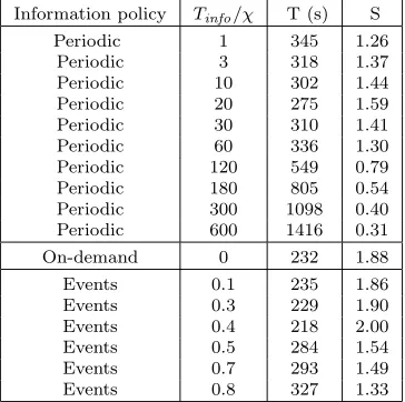
Tables 5.2, 5.3 and 5.4 show the results obtained for experiments 1, 2 and 3. In all these tables the total application response time (T) and the speedup obtained comparing this time with the response time without load balancing algorithm (S) are shown. For the periodic and event-driven policies different values of the information period (Tinf o) and of the event threshold (χ) have been used.
It can be seen that in the low variability environment (experiment 1) the best speedup results are obtained with the event-driven policy, specifically with a threshold value ofχ=0.4 the speedup obtained with the algorithm is 2.00. But the on-demand and periodic policies are able to achieve very similar results, in the case of the periodic approach, with an information interval ofTinf o=20 s, the speedup value is 1.59, and for the on-demand
policy the speedup is 1.88.
Table 5.3
Results for the information rule in experiment 2 (medium variability)
Information policy Tinfo/χ T (s) S
Periodic 1 377 1.32
Periodic 3 354 1.41
Periodic 10 395 1.26
Periodic 20 416 1.20
Periodic 30 459 1.08
Periodic 60 481 1.04
Periodic 120 699 0.71
Periodic 180 993 0.50
Periodic 300 1344 0.37
Periodic 600 1854 0.27
On-demand 0 342 1.46
Events 0.1 276 1.80
Events 0.3 255 1.95
Events 0.4 288 1.73
Events 0.5 376 1.32
Events 0.7 397 1.25
Events 0.8 412 1.21
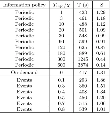
Table 5.4
Results for the information rule in experiment 3 (large variability)
Information policy Tinfo/χ T (s) S
Periodic 1 423 1.29
Periodic 3 461 1.18
Periodic 10 488 1.12
Periodic 20 501 1.09
Periodic 30 548 0.99
Periodic 60 599 0.91
Periodic 120 625 0.87
Periodic 180 889 0.61
Periodic 300 1245 0.44
Periodic 600 3874 0.14
On-demand 0 417 1.31
Events 0.1 293 1.86
Events 0.3 360 1.51
Events 0.4 408 1.34
Events 0.5 456 1.20
Events 0.7 515 1.06
Events 0.8 539 1.01
policy. These best values can be obtained withχ=0.3 andTinf o= 3 s for the experiment 2 and withχ=0.1 and
Tinf o= 1 s for the experiment 3.
The second, the only information policy capable of achieving similar results in the highly variable system than in the low variability environment is the event-driven policy once theχ value is adequately tuned. The speedup decreases only from 2.00 to 1.86 when the variability changes, although the worsening for the on-demand policy is from 1.88 to 1.31 and for the periodic policy is from 1.59 to 1.29.
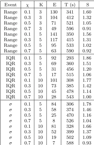
Once the event-driven has been selected to deal with variability, the second set of experiments has been performed to determine the best metric to quantify the workload variability (V) for load balancing purposes. Table 5.5 shows the obtained results using different variability metrics in the experiment 3, the most significative due to its large variability value. Differentχ values for the events definition and different lengths (K) for the vector with the last load index values have been used. The number of information events (and therefore, the number of information messages, directly related to the network overhead), and the total application response time have been measured to evaluate the load balancing algorithm performance,E andT respectively.
Table 5.5
Variability metrics comparison in experiment 3 (large variability)
Event χ K E T (s) S
Range 0.1 3 130 341 1.60 Range 0.3 3 104 412 1.32
Range 0.5 3 71 521 1.05
Range 0.7 3 49 596 0.91
Range 0.1 5 141 350 1.56 Range 0.3 5 117 415 1.31
Range 0.5 5 95 533 1.02
Range 0.7 5 63 590 0.92
IQR 0.1 5 92 293 1.86
IQR 0.3 5 69 360 1.51
IQR 0.5 5 31 456 1.20
IQR 0.7 5 17 515 1.06
IQR 0.1 10 101 308 1.77
IQR 0.3 10 73 385 1.42
IQR 0.5 10 45 478 1.14
IQR 0.7 10 28 543 1.00
σ 0.1 5 84 306 1.78
σ 0.3 5 58 374 1.46
σ 0.5 5 25 470 1.16
σ 0.7 5 8 526 1.04
σ 0.1 10 81 328 1.66
σ 0.3 10 52 399 1.37
σ 0.5 10 19 502 1.09
σ 0.7 10 7 588 0.93
correct load balancing decisions. The range metric can obtain good results in this kind of situation, because there are not important differences between successive load index values. Anyway, this metric may have better performance with lowK values, because the higher this value is the more probability of having measurement errors affecting the variability value (the range increases with the size of the data set as it has been said in section 3.1). On the other hand, the IQR metric can obtain very good results in these environments, even better than the range, because it ignores these extreme values. And finally, the standard deviation is able to obtain similar results than the other two metrics with low variability values.
But the results showed in Table 5.5 are quite different because in this case the system is suffering a high variability. Theχ value which leads to the best response times is very low in all the cases because there are a lot of state changes in the system nodes and therefore, more events and information messages are needed to maintain updated state information and to make correct load balancing decisions.
As it was expected, the range metric performance is very poor in this kind of environment. Even with a lowKvalue, (K=3) the effects of the extreme values on the metric value turns it into a bad election.
However, the IQR metric avoids these problems because it ignores the extreme values. And, furthermore, it can react to unforeseen load changes in a short interval of time, enough to maintain up-to-date state information in almost all the environments. Table 5.5 shows that this metric can obtain the best response time value with an acceptable number of events.
On the other hand, the standard deviation metric suffers the consequences of smoothing the state changes. Its slow variation with the load index changes increases the response time and decreases this metric performance in environments with high variability, because the load balancing decisions are very often based on obsolete state information. The load index changes take longer to have effects on the variability values with this metric than with the range or with the IQR, due to the use of the data arithmetic mean in its calculation and this leads to a low number of events and to a poor information updating.
5.4. Experimental results for the load balancing operation. In these last experiments, the conve-nience of process migration in experiments 1, 2 and 3 has been evaluated using the robustness metrics derived in section 4. In these three experiments the two versions of the load balancing algorithm with the two proposed objectives have been used.
With all the equations proposed in section 4 to perform the robustness analysis, the robustness radius for different system configurations can be theoretically computed.
First, the robustness radius for the load balancing based on the task response time objective can be computed with the QoS-robustness, because it is an objective related to the individual tasks composing the application. The robustness tolerance has been fixed inτR=0.85 and the expected achievement isA=1, therefore:
A≥0.85·A= 0.85.
The application executed in these experiments is composed of 320 tasks, therefore:
A= WC
W =
WC
320 ≥0.85, WC≥320·0.85 = 272, and:
WC=WC−L≥272, L≤48.
The robustness radius for this system-application combination is 48 using the QoS-robustness. On the other hand, if the total response time objective is considered, the P-robustness radius must be computed, because it is a global objective related to the total application. With the same robustness tolerance, the following condition must be fulfilled:
P ≥0.85·P .
In this case, to compute the expected system power:
P =λ· 1
1 + TT, P =λ 1 1 +TT =
320 T ·0.5.
Because in the ideal situationT =T. In the example application the expected response time is T=300 s. Therefore:
P = 0.53.
And the P-robustness condition is in this case:
P ≥0.85·0.53 = 0.45.
Knowing the desired finishing time for all the tasks composing the application, the vectorF can be built. And with this vector and the rest of available information once the application have been executed on the system one time (supposing that there is not a priori information), the robustness radius for all the system nodes can be computed. In this case the minimum robustness radius is the one corresponding to the node n2. For this node the vectorqis:
q2= [2 7 21 34 58 63 94 103 120 193 206 315].
This vector stores the identifiers of all the application tasks allocated to this node, therefore, this node has executed 12 tasks (|q2|= 12) . Using the expression 4.11 for this node and supposing the starting timeTo= 0:
ρ2= 300 0.85√−281
12 = 20.76s with
Table 5.6
QoS-robustness for experiments 1, 2 and 3
Experiment L Kind of system
1 14 QoS-robust
2 20 QoS-robust
3 33 QoS-robust
Table 5.7
P-robustness for experiments 1, 2 and 3
Experiment max(|F(k)−F(k)|) Kind of system
1 6.45 P-robust
2 15.67 P-robust
3 22.45 No P-robust
The meaning of this results is very simple to interpret. In the case of the QoS-robustness, only 48 tasks or less can fail in achieving the objective of having a response time belowtto comply with the robustness condition given in equation 4.1. It has to be pointed that it is a discrete radius because it is a number of tasks.
On the other hand, for the P-robustness the robustness radius is continuous because it is a time measure-ment. The meaning of this radius value is the maximum deviation a task can have from its expected finishing time without causing a violation of the condition given in equation 4.7. Therefore, the maximum difference |F(k)−F(k)|should be 20.76 s to have a robust system-application combination.
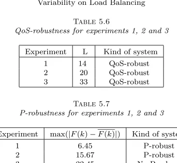
To validate these conclusions, an experimental analysis has been performed. The obtained results are shown in Tables 5.6 and 5.7 for the QoS-robustness and for the P-robustness respectively. Real executions of the studied application have been performed on the Medusa cluster to measure the averageL values (number of tasks that are executed without achieving the desired response time t), the objective achievement value (A), the maximum deviations of the tasks finishing times from their ideal finishing times(max(|F(k)−F(k)|)), the application response time (T) and the system power (P) in experiments 1, 2 and 3. And the conditions expressed in equations 4.1 and 4.7 have been evaluated to verify if the predictions made with the robustness radius about the system robustness are correct.
The results shown in Tables 5.6 and 5.7 verify the proposed robustness metrics and the expressions proposed to compute their associated robustness radius. TheLvalue is always below the QoS robustness radius of 48 and therefore the system is always able to fulfill the robustness condition expressed in 4.1. The same thing occurs with the P-robustness in experiments 1 and 2. But on the other hand, the condition expressed in equation 4.7 cannot be fulfilled for the experiment 3. Therefore, the max(|F(k)−F(k)|) value is above the P-robustness for this experiment and process migration would be needed to achieve the desired system robustness.
6. Conclusions and Future Work. A deep analysis of the effects of variability on load balancing per-formance on cluster systems has been presented. This analysis has demonstrated that these effects are very important for the information rule and the load balancing operation (assuming a good load index selection).
The main contribution of this paper is the proposal of specific solutions for considering the workload variability in this algorithm stage without causing unnecessary overheads on the system nodes or network. These solutions allow to improve the load balancing algorithms performance in highly variable environments such as non dedicated clusters.
For the information rule, an event-driven solution is proposed. The events must be determined with the load index variability on the system nodes. Experimental results have demonstrated that the best variability metric for load balancing purposes is the inter-quartile range (IQR) in all the possible environments. The number of load index values considered for its calculation (K) and the threshold for the information events (χ) must be configured to optimize the load balancing performance depending on the degree of variability and on the executed application.
For the location rule negotiated load balancing operations should be used to give the selected node the chance to reject the operation if its state has changed during the load balancing decisions.
performance. Two new robustness metrics, the QoS-robustness and the P-robustness have been proposed for individual tasks algorithm objectives and for global objectives, respectively.
Both robustness metrics have demonstrated their accuracy in warning the user or administrator when pro-cess migration should be used to manage the workload variability because it is causing intolerable performance degradations. A very interesting line for future research is incorporating the robustness computation to the load balancing algorithm to decide in real-time which distribution rule should be used depending on the workload variability: remote execution or process migration.
REFERENCES
[1] J. Aikat, J. Kaur, F. D. Smith, and K. Jeffay,Variability in TCP round-trip times, in Proceedings of the 3rd ACM SIGCOMM Conference on Internet Measurement, ACM Press, 2003, pp. 279–284.
[2] S. Ali, A. Maciejewski, H. Siegel, and J.-K. Ki,Definition of a robustness metric for resource allocation, in Proceedings of the International Symposium on Parallel and Distributed Processing, 2003, pp. 42–50.
[3] S. Ali, H. Siegel, and A. Maciejewski,The robustness of resource allocation in parallel and distributed computing systems, in Proceedings of the Third International Symposium on Algorithms, Models and Tools for Parallel Computing on Heterogeneous Networks, 2004, pp. 2–10.
[4] T. Anderson and J. D. Finn,The new statistical analysis of data, Springer, 1997.
[5] R. J. Anthony,Self-configuration in parallel processing, in Proceedings of the 16th International Workshop on Database and Expert Systems Applications, 2005.
[6] M. Beltran and J. L. Bosque,Estimating a workstation CPU assignment with the DYPAP monitor, in Proceedings of the Third International Symposium on Parallel and Distributed Computing, 2004, pp. 64–70.
[7] M. Beltr´an, J. L. Bosque, and A. Guzm´an,Initiating load balancing operations, in Proceedings of the EuroPar2005, 2005, pp. 292–301.
[8] M. Beltr´an, A. Guzm´an, and J. L. Bosque,Dealing with heterogeneity in load balancing algorithms, in Proceedings of the Fifth International Symposium on Parallel and Distributed Computing, 2006, pp. 123–132.
[9] R. Buyya,High Performance Cluster Computing: Architecture and Systems, Volume I, Prentice-Hall, 1999.
[10] K.-T. Chen, P. Huang, C.-Y. Huang, and C.-L. Lei,The impact of network variabilities on TCP clocking schemes, in Proceedings of the 4th Annual Joint Conference of the IEEE Computer and Communications Societies, vol. 4, 2005, pp. 2770–2775.
[11] J. J. Evans and C. S. Hood,Network performance variabilty in NOW clusters, in Proceedings of the IEEE International Symposium on Cluster Computing and the Grid, 2005, pp. 1047–1054.
[12] R. Gusella,Characterizing the variability of arrival processes with indexes of dispersion, IEEE Journal on Selected Areas in Communications, 9 (1991), pp. 203–211.
[13] J. L. Hennessy and D. A. Patterson,Computer Architecture: A Quantitative Approach, Morgan Kaufmann, 2003. [14] C. Hughes, P. Kaul, S. Adve, R. Jain, C. Park, and J. Srinivasan,Variability in the execution of multimedia applications
and implications for architecture, in Proceedings of the 28th Annual International Symposium on Computer Architecture, vol. 4, 2001, pp. 245–265.
[15] P. Jogalekar and M. Woodside, Evaluating the scalability of distributed systems, IEEE Transactions on Parallel and Distributed Systems, 11 (2000), pp. 589–603.
[16] D. S. Milojicic, F. Douglis, D. Paindaveine, M. Wheeler, and Z. Zhou,Process migration, ACM Computing Surveys, 32 (2000), pp. 241–299.
[17] R. Mirchandaney, D. Towsley, and J. A. Stankovic,Analysis of the effects od delays on load sharing, IEEE Transactions on Computers, 38 (1989), pp. 1513–1525.
[18] R. Wolski, N. Spring, and J. Hayes,Predicting the CPU availability of time-shared unix systems on the computational grid, in Proceedings of the 8th International Symposium on High Performance Distributed Computing, IEEE, 1999, pp. 105–112.
[19] C. Xu and F. C. M. Lau,Load Balancing in Parallel Computers: Theory and Practice, Kluwer Academic Publishers, 1997.
Edited by: Marek Tudruj, Dana Petcu
Received: January 22th, 2009