Effect of Reynolds Number on Aerodynamic Characteristics of an Airfoil with Flap

Annals of Pure and Applied Mathematics Vol. 3, No. 1, 2013, 27-40

ISSN: 2279-087X (P), 2279-0888(online) Published on 16 May 2013

www.researchmathsci.org

27

Annals of

Effect of Reynolds Number on Aerodynamic

Characteristics of an Airfoil with Flap

1

Md. Hasanuzzaman and 2Mohammad Mashud

1

Department of Mathematics and 2Department of Mechanical Engineering Khulna University of Engineering & Technology

Khulna-9203, Bangladesh Email: mdmashud@yahoo.com

Received 17 April 2013; accepted 25April 2013

Abstract. Over the past few decades due to rapid growth of computer uses and it’s

calculation capability it has been adopted to solve numerical problem by many CFD softwere. By solving Numerical problem thorugh CFD quite accurate and precious result may obtain than laboratory test which is quite expensive. That’s why before work with new design firstly it was tested by numarical method throgh available CFD softwere in computer and based on the result best design is choose to undergo for laboratory test. This reduce time and cost. The goal of this project is to familiar with FLUENT CFD softwere and it’s application. After study flow character stics for varrying Reynolds noumber for an airfoil with and without flap was invistigated. Flow characterstics in terms pressre co-efficient, velocity vector and pressure distribution was observed for varrying Reynolds number. When air flow over airfoil shock wave is formed on it’s upper surface and flow is separated at trailing edge due to adverse pressure gradient. Numerical modelling of 2-D Airfoil without flap and with flap was designed in GAMBIT tool in FLUENT. In this case boundary condition also implimented. Then flow characterstics for designed aifoil was investigated and it is shown graphically at solution steps along with lift and drag plot against angle of attack.

Keywords:Aerodynamic, Airfoil with Flap

AMS Mathematics Subject Classification (2010): 76D99, 76E09

1. Introduction

28

airfoils can generate lift at zero angle of attack. This "turning" of the air in the vicinity of the airfoil creates curved streamlines which results in lower pressure on one side and higher pressure on the other. This pressure difference is accompanied by a velocity difference, via Bernoulli's principle, so the resulting flow field about the airfoil has a higher average velocity on the upper surface than on the lower surface. The lift force can be related directly to the average top/bottom velocity difference without computing.

The pressure by using the concept of circulation and the Kutta-Joukowski theorem [1, 2, 3, 4]. As wing is combination of large number of airfoil, so when air flows over airplane wing it causes airplane to lift. Wing should be proper shape for smooth lift. That’s why airfoil size and shape playing an important role on airplane flying. Plenty of experience was done on effective airfoil design and still it’s modification work is going on. Basic element of an airfoil is shown in Figure 1.

Figure 1: Basic elements of an airfoil

When airfoil moves through air, boundary of air is formed on airfoil surface. Due to presence of friction in air flow causes shear stress at airfoil surface which slow down the air flow near the surface: in the presence of an adverse pressure gradient, there will be a tendency for the boundary layer to separate from the surface. This adverse pressure gradient on top of the airfoil becomes stronger by increase in angle of attack. At stall angle the flow is separated from the upper surface. When the boundary layer separates, its displacement thickness increases sharply, this modifies the outside potential flow and pressure field. In the case of airfoils, the pressure field modification results in an increase in pressure drag and increase loss of lift, all of which are undesirable. So it is desirable to delay the flow separation. The objective of the flow control is to manipulate a particular flow field with a small energy input typically aiming to increase the lift and reduce the drag, to enhance the mixture of momentum, energy, and species, and to suppress the flow-induced noise [5]. The performance and stability of an airplane is often degraded by flow separation. Traditionally, flow separation control is implemented through airfoil shaping, leading edge slat, surface cooling, moving walls, tripping early transition to turbulence, and near-wall momentum addition. Among the near-wall momentum addition methods, steady or pulsed blowing jets and vortex generators (VG) have been widely used [6].

29

30

phenomena in response to actuation have followed. Among the most widely accepted is that unsteady actuation via pulsed blowing, pulsed suction or both (zero net mass flux) is more effective than steady forcing (Seifert et al. 1996). The range of effective dimensionless frequencies associated with this is on the order of unity for which the dimensionless frequency (reduced frequency or Strouhal number), F+, is defined as F+ =

fxsp/U∞ where f is the forcing frequency, xsp is the length of the separated region and U∞ is

the free stream velocity (Darabi and Wygnanski 2004, Glezer et al. 2005). This parameter under scores the importance of the characteristic length scale of separated flow phenomena, xsp,which is the length of the separation zone over the body in question

(Seifert et al. 1996). Physically, the reduced frequency of unity requires that a perturbation must be introduced during the time that the free stream flow propagates over the separated region. The importance of actuator location is closely related to this expression since the shear layer created between the freestream and the low-speed separated region by nature selectively amplifies small perturbations if these are introduced near its receptivity region. The optimum choice of this location for unsteady actuation is generally at or slightly upstream of the separation point. This ensures that the shear layer is excited by the control perturbations near its receptivity point. Successful introduction of such forcing creates large span wise vortices that develop via the Kelvin– Helmholtz instability. These vortices encourage momentum transport between the free stream and the separated region thus reattaching the flow (Darabi and Wygnanski 2004, Melton et al. 2005). Forcing at higher frequencies (F+>10) has been classified as a

different regime and is characterized by enhanced energy dissipation associated with spatial scales in the boundary layer (Amitay and Glezer 2002). Studies on control of trailing edge separation have shown that significantly more momentum in put is required incomparison with leading edge contro (Melton et al. 2006). This is commensurate with the existence of a thicker, likely turbulent boundary layer that develops along the main element of the airfoil. Such results also support leading edge separation control findings that show greater centripetal acceleration created by airfoil surface curvature requires additional momentum for realizing similar control authority (Greenblatt and Wygnanski 2003). Because of these challanges, it is difficult to fully attach the flow over the trailing edge flap. Consequently, both experimental and numerical studies show that lift gains associated with this are often manifested from upstream effects such as an increase in over all circulation (Kiedaisch et al. 2006, Melton et al. 2006). Additional work has shown that the simultaneous use of multiple actuators distributed along the airfoil chord has been more successful than the contribution from each actuator alone (Greenblatt 2007). Not surprisingly, the relative phase between actuator input signals is an important parameter that is highly dependent on the spacing of the actuators, the excitation frequency and the velocity just external to the boundary layer (Greenblatt 2007, Melton et al. 2007).

2. Separation control with DBD plasma actuators

31

relatively new to the aerodynamic community, DBD plasma actuators have long been used in a variety of industrial applications such as ozone generation (Kogelschatz 2003). The use of DBD plasma actuators for airfoil separation control at locations other than the leading edge has been limited. Studies have reported that actuators placed near the trailing edge of airfoils can produce effects similar to plain flaps with deflections of a few degrees (Vorobiev et al. 2008). This results in a uniform increase in lift coefficient across all angles of attack and a slight reduction in minimum drag coefficient, CD, at Reynolds

32

plasma actuation that rely on nano second pulses (Likhanskii et al. 2007, Opaits et al. 2007). These wave forms seem to accomplish control based on thermal effects alone similar to arc filament based plasma actuators (Samimy et al. 2007) and have demonstrated leading edge airfoil separation control authority upto Mach 0.85

(Roupassov et al. 2009) .Because of the amenable characteristics outlined earlier and the variety of parameters that can be explored, plasma actuators continue to be an emphasized point of research in aerospace applications [10].

Another methods of controlling flow separation on high-lift airfoils utilize multi-element flaps that allow mixing of fluid between the pressure and suction sides. Experiments on using flaps at trailing edge shows that as angle between flap and airfoil increases airfoil stall condition also delayed that means flow is controlled.

The objective of this current work is to determine the aerodynamic characterstics for varrying Reynolds number over an airfoil using flap at upper surface by CFD solver. In this experiment NACA 2415 airfoil and FLUENT CFD softwere are used.

Figure 3: Airfoil NACA 2415 Figure 4: Airfoil NACA 2415 with flap

3. Mathematical Modeling

Two equation turbulence models are one of the most common types of turbulence models. Models like the k-epsilon and the k-omega model have become industry standard models and are commonly used for most types of engineering problems. Two equation turbulence models are also very much still an active area of research and new refined two-equation models are still being developed. By definition, two equation models include two extra transport equations to represent the turbulent properties of the flow. This allows a two equation models to account for history effects like convection and diffusion of turbulence energy [11]. Most often one of the transported variables is the turbulent kinetic energy k. The second variable varies depending on what type of two-equation model it is. Common choices are the turbulent dissipation , or the specific dissipation . The second variable can be thought of as the variable that determines the scale of the turbulence (length-scale or time-scale), whereas the first variable k, determines the energy in the turbulence. There are two major formulations of k-epsilon models. The original impetus for the k-epsilon model was to improve the mixing-length model, as well as to find an alternative to algebraically prescribing turbulent length scales in moderate to high complexity flows. The k-epsilon model has been shown to be useful for free-shear layer flows with relatively small pressure gradients. Similarly, for wall-bounded and internal flows, the model gives good results only in cases where mean pressure gradients are small; accuracy has been shown experimentally to be reduced for flows containing large adverse pressure gradients. One might infer then, that the K-epsilon model would be an inappropriate choice for problems such as inlets and compressors.

33

Re = (1)

Continuity equation:

Conservation form

+ . (ρV)=0 (2)

Equation (2) is partial differential equation form of the continuity equation. It was derived on the basis on of an infinitesimally small element fixed in space. The infinitesimally small aspect of the element is why the equation is obtained directly in partial differential form.

Momentum equation:

Navier stocks equation

+ + = − +

+ [μ ( )] + ρF(x) (3a)

+ + = − +

+ [μ( )] + ρF(y) (3b)

Equation of state:

The classic equation of state for an ideal gas,

p=ρRT (4)

Turbulence modeling:

Transport equations for standard k-epsilon model For turbulent kinetic energy

k

k M b k j k t j i i

S

Y

P

P

x

k

x

ku

x

k

t

(

)

(

)

[(

)

]

For dissipation S k C P C P k C x x u x

t j k b

t j i i 2 2 3

1 ( )

] ) [( ) ( )

34

where

]

5

,

43

.

0

max[

C

S

k

In these equations, P_k represents the generation of turbulence kinetic energy due to the mean velocity gradients, calculated in same manner as standard k-epsilon model.

b

P is the generation of turbulence kinetic energy due to buoyancy, calculated in same way as standard k-epsilon model.

Modelling Turbulent Viscosity is

2

k

C

t (8)

where

kU

A

A

C

1

,

U

S

S

~

~

ij ijk ij

ij

2

~

, ij ij ijk ij

and ij is the mean rate-of-rotation tensor viewed in a rotating reference frame with

angular velocity k.

The model constants A0 and As are given by A0 4.04, As 6cos

)

6

(

cos

3

1

W

S S S S

W ij jk ki , S SijSij

~ , ( ) 2 1 j i i j ij x u x u

S (9)

where the model constants are

C

1

.

44

C

1

.

9

1

.

2

4. Numerical Modelling

The solution method utilized for the simulation had a pressure based solver with implicit formulation, 2-D domain geometry, absolute velocity formulation, and superficial velocity for porous formulation. For this test, a simple solver and an external compressible flow model for the turbulence was utilized. The green-gauss cell based was used for the gradient option. There are different equations used for flow and turbulence. A simple method was used for the pressure-velocity coupling. For the discrimination, a standard pressure was used and simulations are 5m/sec and turbulence viscosity ratio is 10. A fully turbulent flow solution was used in ANSYS fluent 6.3.26, where realizable

k-model was used for turbulent viscosity. A simple solver was utilized for the simulation.

5.Computational Domain

35

between the airfoil geometry and the Fairfield boundary. The Fairfield region is created by following measurement:

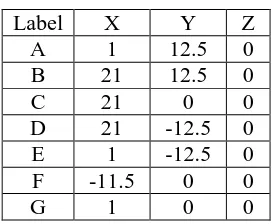
Label X Y Z A 1 12.5 0 B 21 12.5 0 C 21 0 0 D 21 -12.5 0 E 1 -12.5 0 F -11.5 0 0 G 1 0 0

Flow characteristics was determined for given input velocity 4m/s, 5m/s, 6m/s for no flap condition and with flap of 0.15 m long and 0.02m width at at maximum camber position. Successive grid length was 0.96c at all side. Computational domain is divided into 4zones. Ferfield-1, Ferfield-2, Ferfield-3 and Airfoil.

Figure 5: geometry of Airfoil withoutflap Figure 6: Grid for airfoil without flap

Figure 7: geometry of Airfoil with flap Figure 8: Grid for Airfoil with flap

The computational domain was created with 5 face zones and 86460 nodes. The domain is divided in four parts for applying the boundary conditions. These are the airfoil section, farfield 1, farfield 2, and farfield 3. For the airfoil section the solid wall no slip condition was applied. For the farfield 1 boundary condition was velocity inlet and for other two farfields pressure outlet was selected as the boundary condition. The boundary condition for farfield was applied as the velocity components. For X component velocity was applied as 5cos as is the angle of attack. For Y component of velocity 5sin is applied. For the design, mesh generation and applying the boundary condition to the domain to be calculated Gambit was used and Fluent was used as the solver. Fluent has a reliable computational accuracy for fluid flow arrangements and holds good results.

36

computation started and there was a satisfactory output for grid checking for every spoiler position. Convergence criteria were selected as 10-3. This indicates the value taken as the result was constant for consecutive 1000 iterations. Other criterions like continuity residuals were also monitored.

6. Result and Discussion

Figure 9: Lift curve for airfoil without flap Figure 10: Drag curve for airfoil without flap

Airfoil with and without flap for velocity 4 m/s

Figure 13: Comparison of Cl/Cd vs angle of attack for Airfoil with and without flap for velocity 4 m/s

Figure 11: Comparisn of Cl vs angle of atack for Airfoil with and without flap for velocity 4 m/s

37

Figure 16: Comparisn of Cl/Cd vs angle of attack for Airfoil with and witout flap for velocity 5 m/s

Figure 19: Comparisn of Cl/Cd vs angle of attack for Airfoil with and without flap for velocity 6 m/s

Figure 14: Comparisn of Cl vs angle of attack for Aitfoil with and without flap for velocity 5 m/s

Figure 15: Comparisn of Cd vs angle of attack for Aitfoil with and without flap for velocity 5 m/s

Figure 17: Comparisn of Cl vs angle of attack for Airfoil withouit flap and with flap for velocity 6 m/s

38

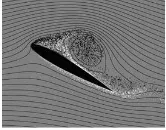
Figure 22: Comparison plot for Cl/Cd vs angle of attack for varying velocity From above figures it’s clear that for varying inlet velocity from 4m/s to 6m/s have shown typical results of Reynolds number effects on lift distribution on airfoil. It’s not difficult to say that as increase in Reynolds number improve the lift and drag characterstics in whole. Form comparison plot for any certain velocity it is seen that lift for airfoil with flap is started incresing from begaing than from no flap condition and drag for flap is always more that without flap. Presence of flap also cause increse of stall angle from no flap condition for a difinite velocity. It has seen that increase of velocity has no effect on stall angle for no flap condition except lift, which is increase as increase in velocity. Different characterstics is visualize from comparison plot for airfoil with flap that increase in vlocity increases lift as well as stall angle. After complete solution of NACA2415 airfoil with flap in FLUENT resultant characterstics plot shows the effect of Reynolds number on pressure distribution on airfoil, the training-edge pressure coefficient and pressure gradient along wall direction which suggests shock wave location and intensity. It can be seen that the upper surface pressure distribution including the location and intensity of shock wave and trailing-edge pressure coefficient, changed apparently with variable Reynolds numbers, while the lower surface pressure distribution is not so sensitive to the Reynolds number. As the Reynolds number increases, the boundary layer of upper surface gets thinner, the location of shock wave moves afterward, intensity of shock wave increases, trailing-edge pressure coefficient improves. From valocity vector and contours of static pressure distribution it’s seen that due to presence of flap flow separats from the surface but reattach with the surface after crossing the flap. As angle of attack increases the possition of reattaching point moves to forward. It’s also seen that at stall condition position of reattaching point moves to left as increase of velocity. This cause increase in lift and delay in flow separation. Thus from

Figure 20: Comparison plot for Cl vs angle of attck for varying velocity

39

results obtained by numerical solution shows that presence of flap increase lift and delay the stall condition which is the basic condition for contrilling flow separation.

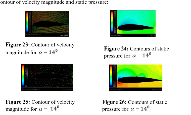
Contour of velocity magnitude and static pressure:

Contour of the velocity magnitude and static pressure for airfoil without flap for angle 140 are shown in the Figures 23 and 24. The effect of the flap is shown by the velocity and the static pressure contour at angle of attact 15 in the Figures 25 and 26. They are the indicate of the changes that occur during the flow over an airfoil section with flap. It is seen that the air flow behind the flap is being disturbed. As the angle of attack increases the region of the negative pressure tends towards the leadind edge and the pressure difference is decreased. Thus the lift force fot the airfoil without any flap is higher than that of the airfoil having a flap. Also the flap resists the flow of the air passing the airfoil, which causes the drag force to be increased.

7. Conclusion

The main objective of this project is to sudy FLUENT CFD softwere and to see effect of reynolds number on aerodynamic characterstics of an airfoil with flap by using this softwere. FLUENT softwere is studied very well including it’s all function and application. From numarical study of arifoil NACA 2415 in FLUENT softwere it’s seen that flow separation can be controle by using flap at maximum camber position.

REFERENCES

1. Halliday, David and Resnick, Robert, Fundamentals of Physics, 3rd edition, John Wiley & Sons.

2. NASA Glenn Research Center, Archived from the original on 5 July 2011, Retrieved

2011-06-29.

3. Weltner, Klaus, Ingelman-Sundberg, Martin, Physics of Flight - reviewed

Figure 23: Contour of velocity

magnitude for = Figure 24: Contours of static pressure for =

Figure 25: Contour of velocity magnitude for =

40

4. Babinsky, Holger (November 2003), How do wings work.

5. M. Serdar Genc, Ünver Kaynak, Control of Laminar Separation Bubble over a NACA 2415 Aerofoil at Low Re Transitional Flow Using Blowing/Suction, 13th International Conference on Aerospace Sciences and Aviation Technology, ASAT- 13, May 26–28, 2009, Paper: ASAT-13-AE-11.

6. Hua Shan, Li Jiang and Chaoqun Liu, Numerical study of passive and active flow separation control over a NACA0012 airfoil, University of Texas at Arlington, Arlington TX 76019, 2007.

7. D.You and P.Moin, Study of flow separation over an airfoil with synthetic jet control using large-eddy simulation, Center for Turbulence Research Annual Research Briefs 2007.

8. M. Serdar Genc and Ünver Kaynak, Control of laminar separation bubble over a NACA2415 aerofoil at low re transitional flow using blowing/suction, 13th International Conference on Aerospace Sciences and Aviation Technology, ASAT- 13, May 26–28, 2009, Paper: ASAT-13-AE-11.

9. Shutian Deng, Li Jiang and Chaoqun Liu, DNS for flow separation control around airfoil by steady and pulsed jets, Department of Mathematics, University of Texas at Arlington, Arlington, TX 76016, USA, Paper presented at the RTO AVT Specialists’ Meeting on “Enhancement of NATO Military Flight Vehicle Performance by Management of Interacting Boundary Layer Transition and Separation”, held in Prague, Czech Republic, 4-7 October 2004, and published in RTO-MP-AVT-111. 10. JesseLittle, Munetake Nishihara, Igor Adamovich and Mo Samimy, High-lift airfoil

trailing edge separation control using a single dielectric barrier discharge plasma actuator, Exp Fluids, 48 (2010), 521–537, DOI10.1007/s00348-009-0755-x, Springer-Verlag 2009.

11. Standard k-epsilon model, CFD-Wiki, the free CFD reference.

12. James E. Fitzpatrick and G. Chested, Furlong-effect of spoiler types lateral-control devices on the TWBTING moments of a wing of NACA 230-series Airfoil Sections- Langle Memorial Aeronautical Laboratory, Langley Field, VA.