1493
Prof. Dr. Marco Wölfle, AFMJ Volume 3 Issue 04 April 2018
Volume 3 Issue 04 April- 2018, (Page No.-1493-1498)
DOI:10.31142/afmj/v3i4.06, I.F. - 4.614
© 2018, AFMJ
Price Bubbles in Real Estate Markets and the Rebound Risk
Prof. Dr. Marco Wölfle
Abstract:
Real estate markets in continental Europe have seen quickly raising prices over the last years. Certainly, low interest rates and extensive credit supply have contributed therefore. As some practitioners fear comparable price cuts as after the subprime bubble in the US, most of the academic literature concentrates on the measurement of price bubbles. This paper, however, does not bring another model to analyze bubble determinants. It focuses on the rebound potential based on a set of data for Germany. While in some scenarios double-digit price cuts result, the majority of the simulations, which can be attributed to moderate increases in the interest rate, yield single-digit reductions. In other words, according to the actual market figures, a bursting German real estate “bubble” would set markets back, to where they were two or three years ago.Keywords
:
Real estate markets, quantitative easing, asset price inflation1. Introduction
Real estate markets in continental Europe have seen quickly raising prices over the last years. Potentially, low interest rates and extensive credit supply have contributed therefore. Certainly, the academic literature is filled with papers on price bubbles in different markets. An actual selection of these is summarized in section 2 of this paper. The literature shows that most research articles support the notion of credit supply in combination with asset price inflation. Consequently, the end of the Quantitative Easing policy runs the risk of dramatic price cuts. While the academic literature focuses on bubble measurement and the identification of determinants, the aim of this paper is to find evidence on the potential consequences of a bursting bubble.
As a proxy for other continental European markets, a set of data for Germany is used to simulate price cuts in real estate markets after a potential increase in the interest rate. While some scenarios see double-digit price cuts, the majority of the simulated results, which can be attributed to moderate increases in the interest rate, yield single-digit reductions. In other words, according to the actual market figures, a bursting German real estate “bubble” would set markets back, to where they were two or three years ago.
2. Literature Review
The evolution of real estate prices is actively discussed in the literature over the last decades. While already Kindleberger (1978) analyzed the relationship between monetary policy and asset price inflation decades ago, recent contributions by O’Meara (2015) as well as Hott / Jokipii (2012) show that real estate price bubbles may be triggered by expansive money supply. Xu and Chen (2012) come to similar conclusions using a Chinese dataset and find that expansive monetary policy lead real estate prices to increase and vice versa. This cyclical behavior can also be seen in
McDonald and Stokes (2013) based on the S&P / Case-Shiller Home Price Index for the US.
Given that most of these studies analyze in a framework of the Taylor Rule, some criticism comes from Brito et al. (2012), who show that real estate prices may also rise quickly although monetary policy is in accordance with the rule, and other authors focus other aspects of monetary policy such as Quantitative Easing (see for example Asadov und Masih (2016) or Favara und Imbs (2015)).
Certainly, other reasons may originate increasing real estate prices such as migration, the relationship between rental rates and purchase prices, increases in the prices for construction materials or market sentiment. For these reasons, the above mentioned and other recent studies have been screened for potential real estate price drivers in order to find a focal point for further analysis.
Table 1. Literature review: Determinants for real estate price increases
Determinants Frequency1
credit supply 10
(expansive) monetary polity 7
ratio rental rate 2
migration 2
construction cost 2 real effective exchange rate 2
media 2
1The figures originate from the following literature contributions
1494
Prof. Dr. Marco Wölfle, AFMJ Volume 3 Issue 04 April 2018
In addition to table 1 the following determinants were mentioned once: risk premia, increases in rental rates, market sentiment, expectation formation, taxes, real income, share prices at the stock exchange, demographics. Quickly, it can be seen, that literature concentrates on monetary policy and credit supply yielding market interest rates, which is also seen as one of the main drivers in the remainder of this paper.
3. Standard Market Model and Real Estate
Markets
Given the Walrasian model, a number of modifications must be made in order to analyze real estate markets. For the standard market setting, reproduction time is usually insignificant and homogeneous goods are traded within a perfect information environment. The standard analysis relies more on arbitrage as on transaction frequency. In contrast to this, real estate is characterized by a high amount of object heterogeneity and an extremely low transaction frequency (Francke / Rehkugler (2011), P. 403). In Germany, average property turnover amounts to more than 42 years (Destatis, 2014) and in general, “producing” new properties needs at least more than two years.
Certainly, in the standard market setting as well as in real estate markets, market equilibrium shows a snapshot, with most potential for a short-run analysis. Moreover, in both situations market participants can only be matched left to the market equilibrium, while some parts of the demand and the supply functions (right to the market equilibrium) remain inactive until the market environment shifts either the demand or the supply function in favor of their market position.
Figure 1. Walrasian market model
Basic microeconomics assumes a clear cut distinction between consumers on the demand side of the market and producers on the supply side of the market. The usual lifecycle of real estate, however, generates a number of inferences to this. One can “consume” real estate either by renting or by owning, so both markets (or parts) show a long-run interaction, since too strong price differentials between rental rates and purchase prices will be substituted away. Moreover, market participants, who in the past acted on the demand side of the market, may get active again on
the supply side, if market conditions change strongly enough. Therefore, observed transaction figures must be interpreted in the context of this double-sided switching potential. A precise measurement on the amount of supplied units of real estate is substituted by an average estimate with a substantial amount of variation.
However, the standard determinants of demand and supply must be specified for real estate markets. Certainly, preferences and income, the main demand drivers are important in real estate markets as well, but suit better for a long-run analysis. Short-run demand for purchasing real estate is mainly driven by the affordability, i.e. the relationship between rental and interest rates. On the supply side of the market, construction does not play the same role as in the general market setting. The number of real estate units is complemented by less than 1% of new units per year.
As in the general market setting, the number of buyers and sellers plays a pivotal role in real estate markets. On a macro level, this may either come by an increasing population due to higher birth rates or by migration from abroad. On a micro level, which shows more effects in the short-run, migration also exists from one municipal area to the next. The German real estate market was characterized over the last years by the so called “swarm theory” (Braun 2017), meaning that two types of people leave rural areas to move to urban areas. First, people some years before retirement prefer a better infrastructure, such as supermarkets, medical facilities and mass transit. Second, young people come to urban areas for their education or study program and stay for their first jobs. Both parts of the trend generate an increase in demand in urban areas regarding the number of apartments, but also an increase in the usage of square meters per person, because this trend goes along with an increase in the number of single households. In rural areas however, the trend reverts to a reduction in demand, and, regarding the older generation moving to the urban area, to an increase on the supply side of the market.
3.1. Residential Property Market in Germany
While the discussion before was focused on the market mechanism on an abstract level, the following discussion aims to describe the market environment and, based on this, to derive the incentive structure of current market participants.
The Federal Statistical Office of Germany (Destatis) differentiates eight groups of property owners. Based on comparable incentive structure, three main groups are summarized and analyzed in the remainder of this paper: Public and non-profit comprising housing cooperations, municipal and national ownership as well as non-profit entities.
1495
Prof. Dr. Marco Wölfle, AFMJ Volume 3 Issue 04 April 2018
Private individuals comprising homeowners as well as private landlords .
German housing cooperations usually calculate cost-oriented rental rates. Therefore their renters are to some extend shielded by changes in demand and supply on the real estate market. Cost-orientation can only yield indirect market influences, if rates for reconstruction increase over time. Non-profit entities are likely to behave in a similar way and rental units under municipal or national ownership are by definition not marked to market. Their aim is to protect specific social classes.
According to the Microzensus 2011 (Destatis 2011), the real estate market in Germany amounts to approximately 40.5 million units. 12.32% fall to group 1 and will not be affected by changes in the market environment.
Group 2 (profit-oriented corporations) however, is closest to the market and amounts to 7.07% of German real estate units. Looking at the transaction volumes (Franke, J. / Lorenz-Hennig, K. 2014), it can be found that units in portfolio transactions vary around 200.000 units per year, which is close to an object turnover between 7% and 10% of the corporate portfolios. This finding is certainly affected by a tax exemption (appreciation is not taxed after 10 years), limited duration of financial credit contracts in Germany, and the typical investment horizon of professional investors. Similarly, their incentive structure is easy to understand. Group 2 compares net rental rates to credit conditions since they invest with high debt-equity-ratios. If central banks’ interest policy changes dramatically, the highest risk is beard by these market participants.
Two types of private individuals exist in group 3 since facing the risk of increasing interest rates, private homeowners will ask themselves, whether they can still serve the interest rate and the repayment for their house, while landlords calculate the rates of their renters plus tax benefits due to depreciation against the interest payment for the credit. According to the Microzensus 2011 private individuals are by far the largest owner group in German real estate markets with 80.61% splitting to 34.38% for homeowners and to 46.32% owing to private landlords. In contrast to profit-oriented corporations, average ownership turnover amounts more than 42 years (Destatis 2014). Comparing the incentives of private landlords to incorporated landlords, their financial structure plays a pivotal role. According to vdp (2017) private individuals buy real estate with an average debt-equity-ratio around 4, while their initial repayment amounts to 2% per year. It can be assumed that corporations show higher debt-equity-ratios and lower repayment.
3.2. Behavioral Model
In order to analyze the market risk due to changing credit conditions the behavioral model for the three groups of market participants is important. First, each group decides about ownership on a regular basis of around 10 years, independently of the average holding period. While
corporations are tied to their investors with a typical investment horizon of 10 years. Both private individuals (homeowners and landlords) have fixed their credit contracts to 10 years, which brings them into a decision situation. Second, beyond the realization of appreciation, corporations and private landlords’ decision between holding or selling looks similar, since it bases on the same determinants, but differentiates on financial conditions.
3.2.1 Profit-oriented Corporations
Given that corporations buy and sell real estate on a regular basis, due to the legal and tax environment as well as investor requirements, it is assumed that sharply rising interest rates will make them more likely to sell real estate. For that reason, the usual corporate turnover, which makes part of the supply side of the market, is increased starting with 10% of their holding.
3.2.2 Private Landlords
Private landlords face a similar decision as corporations, but form a larger share of the real estate market. Given data on debt-equity-ratios by vdp and average interest rates by Deutsche Bundesbank the typical monthly interest payment may be approximated. Consequently, this is linked to the empirica real estate price index (empirica 2017). As private credit duration extends to 10 years, only one tenth of the indebted private landlords will decide yearly about holding or selling property.
3.2.3 Private Homeowners
Private homeowners also decide every ten years, but their basis for decision is whether they can afford the monthly rates given that they should not deviate too much from rental rates.
4. Simulations
4.1 Quantitative Simulations
In order to determine, if a private landlord is likely to sell, the following equation (1) is used as a basis:
r+d≥ i (1)
As long as the interest rate i is less than the rental return r and the tax benefit from depreciation d, the individual landlord will not sell. Given the actual average interest rate for real estate in Germany (2017, October), a depreciation rate of 2%, which is only calculated for the building (on average 80% of the price), but not for land value, equation (1) transmits to
r+1.6%≥ 1.7% (2) r≥ 0.1% (3)
It is easy to see from equation (3), that private landlords will rarely sell their properties. Even when assuming, that they would behave less rational and therefore not observe depreciation, the actual rental returns (empirica 2017) are far beyond the interest rates.
r=2.5%≥ 1.7% (4)
1496
Prof. Dr. Marco Wölfle, AFMJ Volume 3 Issue 04 April 2018
link the figures shown above with credit conditions, however, another modification must be made. Comparing rental returns with interest rates assumes a fully debt-financed property, which is not the case in German real estate markets. As the vdp-data show, average debt amounts to around 80% of the purchase price, while 2% initial annual repayments are fixed over ten years.
r≥ i∙δ+ρ-d (5)
Modifying equation (1) by bringing depreciation to the right side, adding the repayment rate ρ and scaling i with the share of debt in the purchase price δ yields equation (5).
r≥ 1.7%∙0.8+2%-1.6% (6) r≥ 1.76% (7)
Equations (6) and (7) are filled with actual market values to exemplify the minimum return requirement for private landlords under rational expectations. Again a comparison of the 1.76% in equation (7) with market returns is necessary. As long as market returns are significantly higher than this value to compensate for investment risk, private landlords decide for investment and not to sell their property. Given that the actual market returns range between 2.5% and 4.5%, a return differential between 0.74% (= 2.5% - 1.76%) and 2.74% is identical to 100% of the actual number of private landlords. The calculus in the remainder of the paper is done by raising the interest rate in five steps and therefore decreasing the share of private landlords linearly. In order to analyze the market impact of these changes, it has to be noted that private individuals renew their credits every ten years. Consequently, market impact of interest rate increases is scaled down to one tenth. Private homeowners similarly renew their credit after ten years and compare residential expenditures with their income. Given the rates of the social system in Germany, it is assumed that at least 400 € per month are needed to be left over, even after a rise of interest rates. Otherwise, a representative household would be forced to sell his property and become member of the rental market. Destatis (2015) income data is used in combination with the above mentioned changes in the interest rate. The following table 2 gives a summary of the impact:
Table 2. Amount of homeowners selling property due to interest rate changes
Increase interest rate
0.55 %
1.10 %
1.64 %
2.19 %
2.74 %
Quantity
change 0% -17.29% -17.29% -17.29% -48.26%
x 0.1 0% -1.729% -1.729% -1.729% -4.826%
Table 1 shows that homeowners’ decision framework is two-sided. While slight increases in the interest rate will leave the market almost unaffected, sharp rises may yield substantial consequences. The last column of the table
shows that an immediate increase by about 2.74% leads almost every twentieth homeowner to sell his property. Assuming that corporations’ transactions volume increases by 2% for every interest rate step as mentioned in the first row of table 1 and putting together with the shares of the three groups yields a compound selling volume potential as shown in table 3.
Table 3. Potential selling volume due to interest rate changes
Increase interest rate
0.55 %
1.10 %
1.64 %
2.19 %
2.74 %
change 432,191 1,105,408 1,537,599 1,969, 789
2,833,7 05 minus
surplus demand
126,29 1
799,50 8
1,231, 699
1,663, 889
2,527,8 05
4.2 Price Simulations
In order to determine price effects of interest rate changes, the figures in the last row of table 3 need to be linked to marked prices. For 2015, BBSR also offers data on a regional basis, which can be linked to price changes in these regional markets. Therefore the IMV market research database is used as shown in the following table.
Table 4. Regional changes in price due to demand surplus
City Demand surplus Price change
Berlin 1.41% 5.11% Frankfurt 1.04% 1.23% Freiburg 1.50% 1.95% Hamburg 1.34% 2.70% Karlsruhe 1.11% 2.09% Köln 1.00% 2.78% Leipzig 0.69% 6.14% Lörrach 1.17% 6.39% München 1.97% 3.80% Ortenaukreis 0.75% 3.27% Stuttgart 1.33% 2.17%
1497
Prof. Dr. Marco Wölfle, AFMJ Volume 3 Issue 04 April 2018
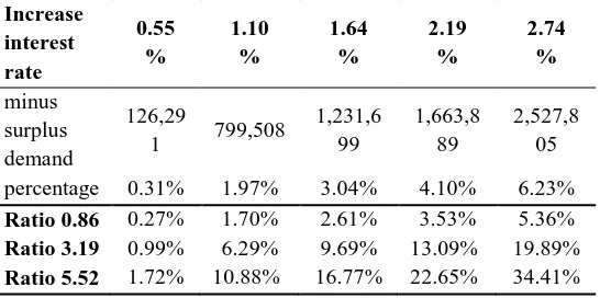
Table 5. Potential price decreases due to interest rateincreases
Increase interest rate
0.55 %
1.10 %
1.64 %
2.19 %
2.74 %
minus surplus demand
126,29
1 799,508
1,231,6 99
1,663,8 89
2,527,8 05
percentage 0.31% 1.97% 3.04% 4.10% 6.23%
Ratio 0.86 0.27% 1.70% 2.61% 3.53% 5.36%
Ratio 3.19 0.99% 6.29% 9.69% 13.09% 19.89%
Ratio 5.52 1.72% 10.88% 16.77% 22.65% 34.41%
Table 5 shows price decreases simulated based on a set of potential interest rate increases. Basically, two dimensions of interpretation exist. On the one hand, market impact depends on the velocity or amplitude of the interest rate change, which is depicted by the columns of the table. On the other hand, the last three rows allow to simulate different scenarios. While an impact ratio of 0.86 assumes a rather conservative market reaction, a ratio of 5.52 means that the market would react very sensitively to interest rate changes. In this latter case, interest rate increases beyond 1% would quickly yield real estate price cuts above 10%.
There exist again two ways to read the table. Looking at the scenarios in the lower right regions of the table, one could conclude to cut down any real estate investment in order to avoid price cuts in the region of 19.89%, 22.65.% or 34.41%. In contrast to this, the majority of the figures in the table ranges in an insignificant dimension. Only 5 of 15 values surpass 10%. In other words, in these cases, real estate prices would fall back to the level, where they were 2 or 3 years ago.
Independent of market sensitivity between 0.86 and 5.52, the dominant question for predicting real estate price reactions is driven by the assumption on interest rate changes. Here however, the central bank policy is important. Most southern European Euro member states show substantial debt ratios. Since rapid raises of interest rates originated from the European Central bank would run these countries into severe financial problems, scenarios in the left columns of table 4 tend to look rather realistic.
4.3. Consequences for Market Participants
As shown in section 4.2 price reductions in real estate markets risk to amount to one third of actual price, when assuming rapid interest rate increases and very sensitive market reaction. Summarizing the results, however, it can be seen that only a minority of the potential scenarios surpasses price cuts of 10%. In most cases, price reductions remain below the price increases of the last two years. Moreover, central bank policy is likely to object rapid and substantial increases in the interest rate in respect of southern European Euro members’ debt policy. Nevertheless, these findings do not release market participants from observing the evolution of interest rates and consecutive market reactions. In
particular, if investment policy is built on raising real estate prices in the future.
5. Conclusions
Researchers and practitioners in the real estate industry both hold low interest rates and credit supply responsible for quickly rising real estate prices. In the light of the experiences during the subprime crisis in the US, some central European markets show strongly rising real estate prices over the last years. Some professionals even fear a similar situation as in the US with price cuts beyond 30%. The simulated results given in this paper point to the notion that double-digit price cuts are not impossible, but rather insignificant price reductions are more realistic facing a potential end of the Quantitative Easing in the monetary policy of the European Central Bank.
Whenever the increase in the interest rate and the decrease in credit supply process moderately, the rebound risk for real estate prices in Germany remains in the single-digit area. In general, two thirds of the scenarios in the paper show price reductions below ten percent. Nevertheless, practitioners building their real estate investment policy on raising prices, should look carefully at central bankers’ decisions and the following market reactions.
References
1. Anundsen, A. K., Gerdrup, K., Hansen, F., Kragh-Sørensen, K. (2016): Bubbles and Crises: The Role of House Prices and Credit, in: Norges Bank: Working Papers, No. 14, p. 1 44.
2. Asadov, A., Masih, M. (2016): Home financing loans and their relationship to real estate bubble: An analysis of the U.S. mortgage market, in: MPRA Paper No. 69771.
3. BBSR (2015): BBSR Wohnungsmarktprognose 2030, Dataset T3.
4. Braun, R. (2017): Lohnt sich eine Immobilie als Kapitalanlage (noch)?, empirica paper No. 238. 5. Brito, P. B., Marini, G., Piergallini, A. (2012):
House Prices and Monetary Policy, in: Studies in Nonlinear Dynamics & Econometrics, No. 20 (3), p. 251 277.
6. Brueckner, J. K., Calem, P. S., Nakamura, L. I. (2012): Subprime mortgages and the housing bubble, in: Journal of Urban Economics, No. 71 (2), p. 230 243.
1498
Prof. Dr. Marco Wölfle, AFMJ Volume 3 Issue 04 April 2018
9. Empirica (2017): Empirica real estate price index, 2017(3).
10. Engsted, T., Hviid, S. J., Pedersen, T. Q. (2016): Explosive bubbles in house prices? Evidence from the OECD countries, in: Journal of International Financial Markets, Institutions and Money, No. 40, p. 14 5.
11. Favara, G., Imbs, J. (2015): Credit Supply and the Price of Housing, in: American Economic Review, No. 105 (3), p. 958 992.
12. Franke, J. / Lorenz-Henning, K. (2014): Transaction volume on residential property in Germany 2014, BBSR-Analysen Kompakt, 2014(10).
13. Destatis (2011): Structural Data on construction and home ownership, Microzensus 2011.
14. Destatis (2014): Structural Data on construction and home ownership, Microzensus 2014, Dataset 2055001149005.
15. Destatis (2015): Household income, Dataset 215010015700.
16. Deutsche Bundesbank (2017): Effective real estate interest rates, 2017, Dataset: BBK01.SUD118. 17. Francke, H.H. / Rehkugler, H. (2011): Real estate
markets and real estate valuation, 2. Edition, Vahlen, München, P. 403.
18. Granziera, E., Kozicki, S. (2015): House price dynamics: Fundamentals and expectations, in: Journal of Economic Dynamics and Control, No. 60, p. 152 65.
19. Griffin, J. M., Maturana, G. (2016): Did Dubious Mortgage Origination Practices Distort House Prices?, in: Review of Financial Studies, No. 29 (7), p. 1671 1708.
20. Hattapoglu, M.; Hoxha, I. (2014): The Dependency of Rent-to-Price Ratio on Appreciation Expectations: An Empirical Approach, in: Journal of Real Estate Finance and Economics, No. 49 (2), p. 185 204.
21. Hott, C., Jokipii, T. (2012): Housing Bubbles and Interest Rates, in: Economic and Social Review, No. 46 (4), p. 521 565.
22. IMV (2017): IMV Marktdaten GmbH, www.immobilien-marktdaten.de.
23. Ling, D. C., Ooi, J. T. l., Le, T. T. (2015): Explaining House Price Dynamics: Isolating the Role of Nonfundamentals, in: Journal of Money, Credit and Banking, No. 47 (1), p. 87 125.
24. Mahalik, M. K., Mallick, H. (2011): What Causes Asset Price Bubble in an Emerging Economy? Some Empirical Evidence in the Housing Sector of
India, in: International Economic Journal, No. 25 (2), p. 215 237.
25. Mercille, J. (2014): The Role of the Media in Sustaining Ireland’s Housing Bubble, in: New Political Economy, No. 19 (2), p. 282 301.
26. McDonald, J. F., Stokes, H. H. (2013): Monetary Policy and the Housing Bubble, in: Journal of Real Estate Finance and Economics, No. 46 (3), p. 437 451.
27. Miranda De Melo, M. (2013): Is There Bubble Price in the Real Estate of Ceara? A Post-Keynesian Approach, in: Transnational Corporations Review, No. 5 (4), p. 96 103.
28. O’Meara, G. (2015): Housing Bubbles and Monetary Policy: A Reassessment, in: The Economic and Social Review,No. 46 (4), p. 521 565.
29. Sá, F. (2015): Immigration and House Prices in the UK, in: The Economic Journal, No. 125 (587), p. 1393 1424.
30. Setzer, R., Greiber, C. (2008): Money and Housing: Evidence for the Euro Area and the US, in: Deutsche Bundesbank Discussion Paper Series 1: Economics Studies, No. 12/2007.
31. Starr, M. A. (2011): Contributions of economists to the housing-price bubble, in: Journal of Economics Issues, No. 46 (1), p. 143 171.
32. Thoma, M. (2013): Bad advice, herding and bubbles, Journal of Economic Methodology, No. 20 (1), p. 45 55.
33. Tokic, D. (2010): The 2008 oil bubble: Causes and consequences, in: Energy Policy, No. 38 (10), p. 6009 6015.
34. Van den Noord, P. J. (2005): Tax Incentives and House Price Volatility in the Euro Area: Theory and Evidence, in: Economie Internationale, No. 101, p. 29 45.
35. Wang, S., Yang, Z., Liu, H. (2011): Impact of urban economic openness on real estate prices: Evidence from thirty-five cities in China, in: China Economic Review, No. 22 (1), p. 42 54.
36. Vdp (2017): vdp spotlight real estate, 2017(10), p. 7.