Journal of Marketing Research
Vol. XLVI (August 2009), 435–445 435
© 2009, American Marketing Association ISSN: 0022-2437 (print), 1547-7193 (electronic)
*Jean-Pierre Dubé is Sigmund E. Edelstone Professor of Marketing (e-mail: [email protected]), Günter J. Hitsch is Associ-ate Professor of Marketing (e-mail: [email protected]), and Peter E. Rossi is Joseph T. and Bernice S. Lewis Professor of Market-ing and Statistics (e-mail: [email protected]), Booth School of Business, University of Chicago. The authors are grateful for comments and suggestions from Matt Gentzkow, Ariel Pakes, Peter Reiss, Alan Sorenson, and Gabriel Weintraub, as well as seminar participants at the University of British Columbia, the University of Chicago structural IO lunch, Duke University, Erasmus University in Rotterdam, Harvard Uni-versity, HEC Montreal, New York UniUni-versity, Northwestern UniUni-versity, the University of Minnesota, University of Rochester, Universiteit van Tilburg, Yale University, the Canadian Competition Bureau, the Chicago Federal Reserve Bank, the 2006 NBER summer IO meetings, the 2006 SED con-ference, the 2007 Summer IO conference at UBC, and Yahoo. Support from the Kilts Center for Marketing, Booth School of Business, University of Chicago is gratefully acknowledged. Tülin Erdem served as guest asso-ciate editor for this article.
The conventional wisdom in economic theory holds that switching costs make markets less competitive. This article challenges this claim. The authors formulate an empirically realistic model of dynamic price competition that allows for differentiated products and imperfect lock-in. They calibrate this model with data from frequently purchased packaged goods markets. These data are ideal in the sense that they have the necessary variation to identify switching costs separately from consumer heterogeneity. Equally important, consumers exhibit inertia in their brand choices, a form of psychological switching cost. This makes the results applicable to the broad range of products that are distinctly identified (i.e., branded) rather than just to products for which there is a product adoption cost or explicit switching fee. In the simulations, prices are as much as 18% lower with than without switching costs. More important, equilibrium prices do not increase even in the presence of switching costs that are of the same order of magnitude as product price.
Keywords: switching costs, dynamic oligopoly, pricing, brand loyalty, competition
Do Switching Costs Make Markets Less
Competitive?
Surveying the theoretical literature on switching costs, Klemperer (1995) and Farrell and Klemperer (2007) con-clude that there is a “strong presumption” that switching costs make markets less competitive. We propose a model with switching costs that can be calibrated from actual con-sumer panel data. For levels of switching costs in our data, we find that equilibrium prices fall in the presence of switching costs. We argue that the conventional wisdom
may not be applicable to empirically relevant models even with high switching costs.
We work with a model that captures the main elements of empirical environments in which switching behavior is observed. Typically, we observe switching costs in markets with differentiated products and with sellers that are not subject to some terminal (i.e., finite horizon) trading period. Switching despite the presence of switching costs is an empirical regularity in many consumer product markets. Often, switching occurs even though the relative prices of products remain roughly constant. Thus, an empirically viable model must allow for differentiated products (in con-trast to Farrell and Shapiro 1988; Padilla 1995) and imper-fect lock-in (Beggs and Klemperer 1992) in an infinite-horizon setting.
Numerical simulations with a simplified version of our empirical model reveal that prices fall for intermediate lev-els of the switching cost compared with an environment with zero switching costs. The incentive for a firm to lower its price and “invest” in customer acquisition is found to outweigh the incentive for a firm to raise its price and “har-vest” its existing customer base. This seemingly counter-intuitive finding reflects the strategic effects of firms lower-ing their prices to defend themselves against other firms’ attempts to steal customers. However, for large enough switching-cost levels, the strategic effects are dampened,
1In previous work (Dubé et al. 2008), we use the same demand specifi-cation to study the category monopolist’s problem. Clearly, competitive forces can alter equilibrium prices as a result of strategic effects; this is the focus here.
and equilibrium prices rise. In general, these preliminary numerical findings suggest that the impact of switching costs on equilibrium prices is an empirical question about the magnitude of switching costs.
Switching costs are typically not directly observed. Instead, the analyst must infer their magnitude from con-sumers’ observed switching behavior. Consumers are also typically heterogeneous in their baseline preferences for products. To separate consumer-specific switching costs from brand preferences, panel data with a long time dimen-sion and some source of exogenous switching are required. Panel data on the purchases of branded, frequently pur-chased products are well suited to this task. Switching costs enter demand models used for these types of products in the same way as in the applied theory literature on switching costs. Frequent price reductions or sales induce switching in the panels, enabling us to identify heterogeneity and switching costs separately. We estimate the demand model from data on two categories of frequently purchased con-sumer products—refrigerated orange juice and margarine— and then compute the price equilibrium.1
We build on a large body of empirical literature that has documented the existence of “brand loyalty” or simply state dependence in consumer choice (Dubé et al. 2008; Erdem 1996; Keane 1997; Roy, Chintagunta, and Haldar 1996; Seetharaman 2004; Seetharaman, Ainslie, and Chintagunta 1999). However, this literature has not explored the impli-cations of state dependence for equilibrium pricing. Che, Sudhir, and Seetharaman (2007) investigate how far bound-edly rational firms look ahead when making pricing deci-sions in markets with state dependence. They do not con-sider how consumer loyalty affects equilibrium prices.
Our work is also related to two recent studies, Doganoglu (2005) and Viard (2007), both of which provide theoretical counterexamples in which switching costs can lower equilibrium prices. However, their examples consist of stylized overlapping generations model specifications chosen on the basis of analytical tractability rather than the ability to produce empirical realistic behavior. In contrast, we work with the classic discrete-choice specification and long-lived consumers, the foundation of the majority of demand systems used in current marketing research and applied industrial organization. We show that switching costs can lower equilibrium prices in the context of state-dependent demand for consumer package goods. In con-trast, Viard’s (2007) empirical results do not contradict the conventional wisdom that switching costs make markets less competitive.
We interpret our estimates of state dependence as arising from a psychological switching cost. Switching costs can come from a variety of sources, including product adoption costs, shopping/search costs, and psychological sources. For example, razor companies create switching costs between brands of razor blades by making handles or razors that fit only their blades. This is one source of switching costs but not necessarily the largest or most uni-versal. The mere purchase/consumption of a distinctly iden-tified (e.g., branded) product can create a switching cost.
Klemperer (1995, p. 518) points this out when he cites “psychological costs of switching, or non-economic ‘brand loyalty’” as an important example of switching costs (see also Farrell and Klemperer 2007). These psychological costs are often believed to come from the well-known phe-nomenon of “cognitive dissonance,” in which consumers change their preferences to “rationalize” previous choices. These psychological sources of switching costs are applica-ble to a much broader array of products than a switching cost narrowly defined as a monetary fee or learning cost. Both psychological switching costs and a monetary switch-ing fee give rise to an observationally equivalent form of inertia in consumer purchases.
Our estimated switching costs are on the order of 15%–19% of the purchase price of the goods. When these switching costs are used in model simulations, equilibrium prices decrease relative to prices without switching costs. This prediction is robust to variation in the parameter val-ues. In particular, if switching costs are scaled up to four times those inferred from our data, we still find that prices decline. We observe price reductions of up to 18% in the presence of switching costs.
THE MODEL
The model consists of single-product firms competing for consumers with switching costs by pricing differenti-ated products. Each firm sets a pricing policy to maximize the discounted sum of profits over an infinite horizon. The solution concept for this game is Markov perfect equilib-rium (MPE). The goal is to study the effects of consumer switching costs on pricing in the context of a model that generalizes much of the empirical research on differentiated products demand estimation. Unlike much of the estab-lished theoretical literature, we allow for product differenti-ation and imperfect lock-in—the possibility that consumers switch away from products they have previously pur-chased—which are features commonly present in actual markets. In addition, we include a random utility compo-nent, which allows for the possibility that consumers switch products even when relative prices are not changing.
We emphasize that our research focuses on markets in which switching costs are actual opportunity costs to con-sumers, not on markets with customer recognition in which firms charge different prices to new and previous cus-tomers. In the literature on customer recognition, unlike in the literature on switching costs, it is well established that equilibrium prices can be lower than if firms are unable to price discriminate between new and old customers (for a survey, see Fudenberg and Villas-Boas 2006).
After developing the model in general, we briefly explore a simple case to illustrate how the features of con-sumer choice influence pricing in the presence of switching costs. The advantage of this model is that it simplifies com-putation of an equilibrium, which means that we can easily explore several comparative static exercises.
DEMAND
Demand is derived from a population of consumers who make discrete choices from J product alternatives and an outside option (i.e., no-purchase). For simplicity, we drop the consumer-specific index. In each period t, a consumer is loyal to one product, st∈{1, …, J}. If the consumer is
cur-rently loyal to product j, st= j, and purchases product, k ≠j,
then his or her loyalty state changes, st + 1= k. If the
con-sumer chooses product j or the outside option, then st + 1=
st(i.e., the consumer’s brand loyalty remains unchanged).
Conditional on price pjtand the consumer’s current loyalty
state st, the utility index from the choice of a product j at
time t is as follows:
The demand model in Equation 1 has been used extensively in the empirical literature on consumer package goods (Erdem 1996; Keane 1997; Shum 2004). We assume that the random utility component, εjt, is i.i.d. Type I extreme
value distributed. If the consumer is loyal to j but buys product k ≠j, he or she forgoes the utility component γ. Thus, the consumer implicitly incurs a switching cost. Note that the consumer behavior associated with switching cost/product loyalty, γ, is different from the consumer behavior associated with the brand intercept, δj. An
increase in the brand intercept always increases the proba-bility of purchase of the jth brand, while the switching-cost parameter increases only the purchase probability if the consumer is currently loyal to j.
Let U(j, st, p) denote the deterministic component of the
utility index, such that ujt= U(j, st, p) + εjt. The utility from
the outside alternative is U0t= U(0, st, pt) = ε0t. The
con-sumer’s choice probability has the following logit form:
Demand parameters in Equation 2, θ= (δ1, …, δJ, α, γ),
are consumer specific with N “types” in the market. The behavior of each consumer type n is fully summarized by the taste vector, θn. For example, the probability that a
con-sumer of type n in state stwill buy product j is denoted by
Pj(st, pt; n). We assume that for each consumer type, there
is a continuum of consumers in the market with mass μn.
At any point in time, the market is summarized by the distribution of consumers over types and loyalty states. Let be the fraction of consumers of type n who are
loyal to product j. The vector
summa-rizes the distribution over loyalty states for all consumers of type n, and (x1
t, ..., xtN) summarizes the state of the whole
market, where X denotes the state space.
We obtain aggregate demand by summing consumer-level demand over consumer types and loyalty states. Aggregate demand for product j is given by the following:
Evolution of the State
The distribution of consumer loyalty states, xt= (x1t, ...,
xtN), summarizes all current-period payoff-relevant
informa-tion for the firm and describes the state of the market. The transition of the aggregate state can be derived from the transition probabilities of the individual states. Conditional on a price vector pt, we can define a Markov transition
matrix Q(pt; n) with the following elements:
( )3 ( , ) ( , ; )
1
D xj t pt n x P k pktn n j t k J = ⎡ ⎣ ⎢ ⎢
∑
= μ ⎤⎤ ⎦ ⎥ ⎥ =∑
n N 1 . xtn=(x1nt, ..., xJtn) xnjt ∈[ , ]0 1( ) ( , ) exp[ ( , , )] exp[ ( , ,
2 P s p U j s p
U k s j t t
t t t = pt k J )] . =
∑
0( )1 ujt =δj+αpjt+γI s
{
t≠ j}
+εjt.2This assumption rules out behavior that conditions current prices also on the history of past play and, thus, collusive strategies in particular. where
Here, Qjk(pt; n) denotes the probability that a consumer of
type n who is currently loyal to product k will become loyal to product j. The whole state vector for type n then evolves according to the Markov chain:
Consumers can change loyalty states but not types, such that the overall market state vector xtalso evolves
accord-ing to a Markov chain with a block diagonal transition matrix. The evolution of the state vector is deterministic, and we denote the transition function by f, xt + 1= f(xt, pt).
Firms
We consider a market with J competing single-product firms. Time is discrete, t = 0, 1, …. Conditional on all prod-uct prices and the state of the market, xt, firm j’s
current-period profit function is πj(xt, pt) = Dj(xt, pt) ×(pj – cj),
where cjis the marginal cost of production, which does not
vary over time. Firms compete in prices and choose Mar-kovian strategies, σj: X →⺢, that depend on the current
payoff-relevant information, summarized by x.2Firms
dis-count the future using the common factor β, 0 ≤β< 1. For a given profile of strategies, σ= (σ1, …, σJ), the present
discounted value of profits, , is well
defined. Conditional on a profile of competitors’ strategies, σ–j, firm j chooses a pricing strategy that maximizes its
expected value. Associated with a solution of this problem is firm j’s value function, which satisfies the Bellman equation
In this equation, the price vector consists of firm j’s price and the prices prescribed by the competitors’ strategies, p = [σ1(x), …, σj – 1(x), pj, σj + 1(x), …, σJ(x)]. Therefore, the
Bellman equation (Equation 5) depends on the pricing strategies the competitors choose.
We use MPE as our solution concept. In pure strategies, MPE is defined by a pricing strategy for each firm, and an associated value function, Vj, such that
for all states, x, and firms. That is, in each subgame starting at x, the firm’s strategy is a best response to the strategies its competitors choose. For a simple version of the model, which we explore in the next section, we can prove the
V xj p jx pj j x V f x pj j
j
( )=max [ , , * ( )]+ { [ , , −
ω σ β σσ−
(
*j( )]}x)
σ*j, ( )5 ( ) max ( , ) [ ( , )]
0
V xj x p V f x p x
pj j j
=
{
+}
∀≥ π β ∈∈X.
β πt σ
t= jxt xt
∞
∑ 0 [ , ( )]
xtn Q p n x t nt
+1= ( ; ) .
( ) Pr{ , , }
( , ; ) ( ,
4 1
0
s j s p n
P s p n P s
t t t
j t t t
+ =
= +
| p
p n j s
P s p n j s
t t
j t t t
; ) , ( , ; ) . if if = ≠ ⎧ ⎨ ⎪ ⎩⎪
3Even in static games of price competition, restrictions on the distribu-tion of consumer tastes need to be imposed to establish the existence of a pure strategy equilibrium (Caplin and Nalebuff 1991). In general, the “nonparametric” distribution of tastes that our model allows for does not obey these restrictions.
existence of a pure strategy price equilibrium. However, we cannot prove that a pure strategy equilibrium exists in gen-eral.3We establish the existence of a pure strategy
equilib-rium computationally on a case-by-case approach. In Web Appendix A (http://www.marketingpower.com/jmraug09), we describe the numerical algorithm used to compute the price equilibrium.
A SIMPLIFIED MODEL
We briefly consider a simplified variant of the model dis-cussed in the previous section for the purpose of building an intuition as to why switching costs can lead to lower equilibrium prices. Subsequently, we return to the model with many consumer types and base our pricing computa-tions on empirical estimates of this model.
We assume that there is exactly one consumer in the market, who chooses among the J products and an outside option in each period, as in Equation 1. With only one con-sumer, equilibrium computations are simplified greatly, facilitating the comparative statics necessary to develop an intuition regarding the role of switching costs. Here, we are following several recent studies that use computational methods to establish properties of various theoretical mod-els (Besanko et al. 2007; Doraszmod-elski and Satterthwaite 2005).
The loyalty variable of this consumer, st∈X = {1, …, J}
summarizes all current-period payoff-relevant information and describes the state of the market. Conditional on all product prices and the state of the market, firm j receives the expected current-period profit πj(st, pt) = Pj(st, pt) ×
(pjt– cj). Although we can show the existence of a
pure-strategy equilibrium (see Web Appendix B1 at http://www. marketingpower.com/jmraug09), we cannot characterize the equilibrium policies analytically. Instead, we solve the game numerically for different parameter values. Motivated by the current research, Cabral (2009) derives theoretical results that support our computations.
We now explore the predictions of the simplified pricing model. To keep the exposition as simple as possible, we focus on symmetric games with two firms. Each firm has the same utility intercept and marginal production cost. In a
symmetric equilibrium, and
Therefore, we only need to know firm 1’s pricing policy to characterize the market equilibrium.
We first consider the case of homogeneous products (i.e., with εjt= 0). In this case, we can establish theoretically (see
Web Appendix B2 at http://www.marketingpower.com/ jmraug09) that switching costs enable firms to raise prices above the baseline Bertrand outcome, where p = c. In par-ticular, there is an equilibrium in which the firm that pos-sesses the loyal customer increases its price above cost by the value υ= (1 – β)γ, where υis the flow value of the switching cost. If the firm charges an even higher price, the competitors could poach the customer by subsidizing the switching cost, incurring a loss in the current period, and σ1*( )2 =σ1*( ).1
σ1*( )1 =σ*2( )2
recouping this loss by pricing above cost in the future. In summary, if products are not differentiated, we find that switching costs make markets less competitive, as much of the previous literature predicts.
We now turn to the case of differentiated products and switching in equilibrium. In the case of product differentia-tion, the customer sometimes switches, and therefore we characterize the equilibrium outcome by the average trans-action price paid, conditional on a purchase:
That is, pais the expected price paid in state s
t= 1, which,
due to symmetry, is the same as the expected price paid in state st= 2. In addition, P1(·, ·), P2(·, ·) are the probabilities
of choice of each product conditional on price and loyalty state.
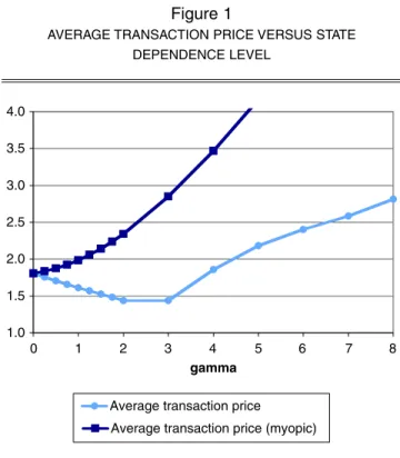
Figure 1 shows the relationship between the level of switching costs and the average transaction price for the case of δj= 1, cj= .5, α= 1. We find that prices initially fall
and then rise for larger switching-cost levels. Indeed, only for switching-cost levels larger than 4 does the average transaction price exceed the transaction price without switching costs. Though not reported, we find that the main result—that prices are decreasing and then increasing in the level of γ—is robust to the exclusion of the outside good and to the degree of switching (the scale of the intercept and price coefficients in Equation 1). These results show that the conjectured effect of switching costs on prices— switching costs make markets less competitive—need not be true in a model that is a simplified variant of a widely used class of empirical demand models.
To understand our results, recall that under competition with switching costs, firms face two incentives that work in opposite directions (Klemperer 1987). First, firms can
har-p P P
P
a = 1[ ,1 σ*( )]1 ×σ*1( )1 + 2[ ,1 σ*( )]1 ×σ*2( )1 1
1[ ,1 ( )]1 2[ ,1 ( )]1 .
* *
σ +P σ
1.0 1.5 2.0 2.5 3.0 3.5 4.0
0 1 2 3 4 5 6 7 8
gamma
Average transaction price Average transaction price (myopic)
Figure 1
AVERAGE TRANSACTION PRICE VERSUS STATE DEPENDENCE LEVEL
vest a loyal customer by charging higher prices. Second, firms can invest in future loyalty by lowering current prices. Our results imply that either force can dominate in equilib-rium. Imperfect lock-in (γ< ∞) and the random component in consumer tastes, features common to many empirical models of differentiated products demand, stimulate the incentive to cut prices to attract competitors’ loyal cus-tomers. Anticipating this incentive, the competitors lower their price to prevent the customers from switching. In some instances, this downward pressure on prices over-shadows the upward pressure from harvesting. In contrast, Beggs and Klemperer (1992) consider only the case of per-fectly locked-in consumers (γ= ∞). In their specification, the incentive to harvest always outweighs the incentive to invest.
To illustrate the role of the investment motive, we exam-ine the extreme case in which only the harvesting incentive is present. To exclude the investment motive, we consider competitors that do not anticipate the future benefits from lowering current prices and thus set prices myopically (β= 0). Figure 1 shows the average transaction price paid under this scenario; this enables us to compare the pricing out-comes for fully rational, forward-looking firms and myopic decision makers. After the investment motive is eliminated, prices always rise in the degree of switching costs—that is, switching costs make markets less competitive. In general, the average transaction price under competition with forward-looking firms is always lower than the average price under myopic competition.
One of the difficulties in interpreting the comparative static result displayed in Figure 1 is that an increase in γnot only increases the switching cost but also leads to an increase in the total market size (i.e., a decrease in the out-side good share). Because our interest lies in the role of switching behavior, we construct an adjusted comparative static exercise in which γ does not influence the outside share and leaves the total market size constant. Table 1 indi-cates that we still observe the main result of decreasing-then-increasing prices. In addition, it reports the probability
that the consumer will remain loyal. Note that even when the consumer will remain loyal with probability .981, equi-librium prices are still below those that would occur with-out switching costs. This suggests that results in the litera-ture (i.e., prices rise) are closely linked with assumptions of perfect lock-in.
In Table 2, we report the impact of switching costs on firm profits. We consider profits from both the oligopolistic equilibrium prices and profits that would occur if prices were fixed at the levels obtained under zero switching costs (γ = 0). These profit values appear in the right-most two columns of the table. In this latter scenario, the firm with the loyal customer is strictly better off when the switching cost increases. However, when the firms reoptimize their prices, both firms can be strictly worse off if the switching cost leads to lower equilibrium prices. That is, if prices are held constant, the strategic effect of price competition on profits outweighs the direct effect of switching costs on profits. Thus, the investment motive under competition out-weighs the harvesting incentive. This outcome is an instance of a “Bertrand supertrap,” as analyzed by Cabral and Villas-Boas (2005) for finite-horizon games.
In Web Appendixes D and E (see http://www.marketing power.com/jmraug09), we discuss two additional variants of the simple model to check the robustness of our results to other model features typically considered in the theo-retical literature. We consider separately the impact of forward-looking consumer behavior and overlapping gener-ations of consumers on equilibrium prices. The main con-clusion—that switching costs do not necessarily lead to higher prices—is robust to these different model formula-tions and to a wide range of parameter values.
In summary, we show that contrary to the conventional wisdom, switching costs can toughen price competition. We also show that this result arises from the dynamics associ-ated with the investment motive. In particular, when there is some random switching in equilibrium, firms may compete both to attract and to retain the customer. When the strate-gic effects are large enough, they can cause the investment
Table 1
EQUILIBRIUM PRICES UNDER DIFFERENT SWITCHING-COST LEVELS
Switching Purchase Purchase Probability of
Cost p1 p2 pa Probability 1 Probability 2 Staying Loyal
.00 1.808 1.808 1.808 .236 .236 .764
.25 1.802 1.658 1.734 .258 .232 .768
.50 1.794 1.500 1.662 .279 .227 .773
.75 1.784 1.335 1.593 .298 .221 .779
1.00 1.773 1.165 1.528 .317 .214 .786
1.25 1.762 .991 1.467 .334 .207 .793
1.50 1.750 .813 1.410 .349 .199 .801
1.75 1.738 .631 1.356 .363 .191 .809
2.00 1.727 .445 1.307 .376 .183 .817
3.00 1.732 .000 1.352 .421 .119 .881
4.00 1.782 .000 1.607 .450 .049 .951
5.00 1.812 .000 1.740 .460 .019 .981
6.00 1.844 .000 1.816 .458 .007 .993
7.00 1.896 .000 1.885 .448 .003 .997
8.00 1.972 .000 1.967 .430 .001 .999
Notes: For positive switching-cost levels, δis adjusted so that the total market size remains constant (for the details, see Web Appendix C at http://www.marketingpower.com/jmraug09). We calculated the results for product intercepts = 1.0 and a price coefficient = 1.0, as well as for an outside good intercept at 0. The discount factor is β= .998.
Table 2
FIRM PROFITS UNDER DIFFERENT SWITCHING-COST LEVELS
Switching
Cost pa V
1 V2 V
0
1 V
0 2
.00 1.808 154.1 154.1 154.1 154.1
.25 1.734 151.0 150.8 154.2 154.0
.50 1.662 146.9 146.6 154.3 153.9
.75 1.593 142.1 141.6 154.5 153.8
1.00 1.528 136.7 136.1 154.7 153.6
1.25 1.467 131.0 130.2 154.9 153.3
1.50 1.410 125.1 124.2 155.3 153.0
1.75 1.356 119.2 118.1 155.7 152.6
2.00 1.307 113.4 112.1 156.2 152.1
3.00 1.352 116.2 113.8 160.1 148.1
4.00 1.607 141.2 135.1 169.8 138.4
5.00 1.740 156.1 140.8 190.8 117.5
6.00 1.816 172.1 134.2 225.0 83.2
7.00 1.885 198.2 113.8 261.8 46.4
8.00 1.967 236.1 80.3 287.2 21.1
Notes: For positive switching-cost levels, δis adjusted so that the total market size remains constant (for the details, see Web Appendix C at http://www.marketingpower.com/jmraug09). We calculated the results for product intercepts = 1.0 and a price coefficient = 1.0. The term Vjdenotes the value of firm j in state 1, and V0jdenotes the value of firm 1 in state s if prices remain constant at their no-switching-cost level, p1= p2= 1.808.
4Though not reported, our findings are robust to the inclusion of promo-tional variables, such as weekly product features and in-aisle displays. motive to outweigh the harvesting motive, leading to lower equilibrium prices. In the next section, we investigate whether this result still holds when we consider a richer model that generalizes much of the empirical research on demand estimation.
EMPIRICAL MODEL AND ESTIMATION
We now explore the impact of consumer switching costs on our full model with many “types” of consumers. Recall that for the simple version of the model with a single con-sumer, we observed that equilibrium prices can be lower with than without switching costs for a wide range of parameter values. Therefore, the impact of switching costs on prices is an empirical matter regarding the magnitude of switching costs consistent with actual consumer behavior. Thus, we calibrate our analysis of the full model using actual empirical estimates of the joint distribution of prefer-ences and switching costs, θ, for a population of heteroge-neous consumers. In the subsequent sections, we describe the data and the procedure used to estimate the demand parameters.
Econometric Model
For the full model, the probability that consumer h chooses alternative j given loyalty to product k is given by the following:4
( ) ;
exp { }
exp 6
1 P j s k
p I s j
h j
h h j h
| =
(
)
=(
+ + =)
+
θ δ α γ
δδhj αh j γh
k J
p I s k
+ + =
(
)
=
∑
{ }. 1
It might be argued that the switching cost, γh, could be
modeled using a much more complex function of a con-sumer’s purchase history. However, as we discussed previ-ously, there is a well-established precedent for using this specification in the empirical literature devoted to package goods demand. Furthermore, this specification is identical to the one routinely used in the applied theory literature on switching costs. Other specifications of switching costs or state dependence involve more general functions of past choices. Although these specifications can be easily esti-mated (see Dubé, Hitsch, and Rossi 2008), computing equi-librium prices may be difficult because of an increase in the dimension of the state space required.
To accommodate differences across consumers in Equa-tion 6, we use a potentially large number of consumer types and a continuum of consumers of each type. A literal inter-pretation of this assumption is that the distribution of demand parameters is discrete but with a large number of mass points. In the consumer heterogeneity literature (Allenby and Rossi 1999), continuous models of hetero-geneity have gained favor over models with a small number of mass points. The distinction between continuous models of heterogeneity and discrete models with a large number of mass points is largely semantic. Even some nonparamet-ric methods rely on discrete approximations. Our approach is to specify a flexible but continuous model of heterogene-ity and then exploit recent developments in Bayesian infer-ence and computation to use draws from the posterior of this model as “representative” of the large number of con-sumer types. Each concon-sumer in our data is viewed as repre-sentative of a type. We use Markov chain Monte Carlo (MCMC) methods to construct a Bayes estimate of each consumer’s coefficient vector.
Our approach is to use a mixture of normals as the distri-bution of heterogeneity in a hierarchical Bayesian model. With sufficient components in the mixture, we can accom-modate deviations from normality, such as multimodality, skewness, and fat tails. Let θhbe the vector of choice model
parameters for consumer h. The mixture-of-normals model specifies the distribution of θhacross consumers as follows:
where πis a vector giving the mixture probabilities for each the K components. We implement posterior inference for the mixture-of-normals model of heterogeneity and the multinomial logit base model along the lines of Rossi, Allenby, and McCulloch’s (2005) work.
Our MCMC algorithm provides draws of the mixture probabilities and the normal component parameters. Thus, each MCMC draw of the mixture parameters provides a draw of the entire multivariate density of consumer parame-ters. We can average these densities to provide a Bayes esti-mate of the consumer parameter density. We can also con-struct Bayesian credibility regions for any given density ordinate to gauge the level of uncertainty in the estimation of the consumer distribution. In Dubé, Hitsch, and Rossi (2008), we provide a wide variety of models with different specifications of the number of normal components as well as heterogeneity and various robustness checks of the basic state-dependent specification.
θ μ
π
h
ind ind N
ind
~ ( , )
~multinomial( ),
Description of the Data
Switching costs are rarely directly observed (some com-ponents may be known, but the “hassle” costs of switching are not). For this reason, we must turn to data on the pur-chase histories of customers to infer switching costs from the observed patterns of switching between brands in the face of price variation. Consumer panel data on the pur-chases of packaged goods are ideal for estimating switching costs. The panel length is long relative to the average inter-purchase times, and there is extensive price variation that causes frequent brand switching, thus generating variation in consumers’ loyalty states.
For our empirical analysis, we estimate the logit demand model we described previously using household panel data that contain all purchase behavior for the refrigerated orange juice and the 16-ounce tub margarine categories. The panel data were collected by ACNielsen for 2100 households in a large midwestern city between 1993 and 1995. In each category, we focus only on households that purchased a brand at least twice during our sample period. Thus, we use 355 households to estimate orange juice and 429 households to estimate margarine demand. Table 3 lists the products considered in each category as well as the pur-chase incidence, product shares, and average retail and wholesale prices.
More than 85% of the trips to the store recorded in our panel data do not involve purchases in the product category. However, it is unlikely that each observed trip to the super-market potentially results in the purchase of either a pack of refrigerated juice and/or a tub of margarine. For a more realistic analysis, we define the outside good in each cate-gory as follows: In the refrigerated orange juice catecate-gory, we define the outside good as any fresh or canned juice product purchase other than the brands of orange juice con-sidered. In the tub margarine category, we define the out-side good as any spreadable product (e.g., jams, jellies,
margarine, butter, peanut butter). Table 3 shows that under these definitions of the outside good, there is a no-purchase share of roughly 24% in refrigerated juice and 46% in tub margarine.
Demand Estimates
We now report the empirical estimates of demand from the orange juice and margarine data. We emphasize that our model includes heterogeneity in all parameters: intercepts, price coefficient, and switching-cost terms. Our procedure provides a fitted density of model parameters across all panelists. We report various marginals of this joint distribu-tion to show the need for flexibility in modeling hetero-geneity and then to cluster the household posterior mean coefficients for use in our equilibrium pricing implications. A model with a switching-cost term fits the data with a much higher likelihood and posterior model probability than a heterogeneous model without switching costs (for detailed model comparisons, see Dubé, Hitsch, and Rossi 2008). Because our model of heterogeneity is flexible, we are confident that we are capturing true state dependence (switching costs) and that this is not an artifact of making an arbitrary distribution assumption regarding tastes (e.g., the normal used in the literature).
Figures 2 and 3 plot several fitted densities from the one-and five-component mixture models for a subset of the model parameters. We also report the 95% posterior credi-bility region (the yellow envelope) for the five-component mixture model. The region constructed around the marginal from a five-component fit can be used to make inferences about the differences between normal and nonnormal assumptions. Figures 2 and 3 provide compelling evidence of the need for a flexible model that is capable of
address-Table 3 DESCRIPTION OF DATA A: Refrigerated Orange Juice
Retail Wholesale
Product Price Price Trips (%)
64-ounce Minute Maid 2.21 1.36 11.1
Premium 64-ounce Minute Maid 2.62 1.88 7.00
96-ounce Minute Maid 3.41 2.12 14.7
Premium 64-ounce Tropicana 2.73 2.07 28.80
64-ounce Tropicana 2.26 1.29 6.76
Premium 96-ounce Tropicana 4.27 2.73 7.99
No purchase (% trips) 23.75
Number of households 355.00
Number of trips per household 12.3 Number of purchases per household 9.37
B: Margarine
Promise 1.69 1.22 13.11
Parkay 1.63 1.02 4.98
Shedd’s 1.07 .83 12.66
I Can’t Believe It’s Not Butter! 1.55 1.11 23.51
No purchase (% trips) 45.73
Number of households 429.00
Number of trips per household 18.25 Number of purchases per household 9.90
–15 –10 –5 0 5 10 15
beta
One-component model Five-component model .20
.10
.00
One-component model Five-component model
–10 –5 0 5
beta
.2
.0
Figure 2
FITTED DENSITIES FOR I CAN’T BELIEVE IT’S NOT BUTTER! BRAND INTERCEPT AND PRICE COEFFICIENT
A: I Can’t Believe It’s Not Butter!
Figure 3
FITTED DENSITIES FOR 64-OUNCE PREMIUM TROPICANA BRAND INTERCEPT AND PRICE COEFFICIENT
A: 64-Ounce Premium Tropicana
–2 0 2 4 6 8 10
.20 .10 .0
One-component model Five-component model
beta
–3 –2 –1 0
.6 .4 .2 .0
One-component model Five-component model
beta
B: Price
Figure 4
FITTED DENSITIES AND 95% POSTERIOR CREDIBILITY REGIONS FOR THE MONEY-METRIC STATE DEPENDENCE
PREMIUM IN DOLLARS (MARGARINE)
–2 0 2 4
.5
.4
.3
.2
.1
.0
Switching Cost Premium ($)
Five-component model No heterogeneity
–1 0 1 2
.6
.5
.4
.3
.2
.1
.0
Switching Cost Premium ($)
Five-component model No heterogeneity
Figure 5
FITTED DENSITIES AND 95% POSTERIOR CREDIBILITY REGIONS FOR THE MONEY-METRIC STATE DEPENDENCE
PREMIUM IN DOLLARS (ORANGE JUICE)
ing nonnormality. In Panel A of both figures, the intercepts from one of the popular brands exhibit a bimodal distribu-tion that cannot be captured by the normal (one-component) model. The bimodality implies that there are households that differ markedly in their quality perceptions for margarines. In Figure 2, the price coefficient for mar-garine has a skewed and bimodal density. The symmetric one-component model has both a mode and tails lying out-side the credibility region for the five-component model. In general, the results suggest that there would be a mislead-ing description of the data-generatmislead-ing process if the usual symmetric normal (one-component) prior were used to fit these data.
Figures 4 and 5 display the fitted densities of the switching-cost premium in dollar terms for each category. The inclusion of the outside option in the model enables us to assign money-metric values to our model parameters simply by rescaling them by the price parameter (i.e., the marginal utility of income). For the switching-cost parame-ter reported in the figures, this ratio represents the dollar cost forgone when a consumer switches to another brand rather than the one purchased previously. In the graphs, we denote the point estimate of switching costs from the homogeneous logit specification with a vertical solid line.
Figures 4 and 5 display an entire distribution of switch-ing costs across the population of households. Some of the values on which this distribution puts substantial mass are rather large values; others are small. To provide some sense of the magnitudes of these values, we compute the ratio of the dollar switching cost to the average price of the prod-ucts. The ratio of the mean dollar switching cost to the average price is .19 for margarine and .15 for orange juice.
We emphasize that the entire distribution of switching costs will be used in computation of equilibrium prices. The
dis-5In a companion paper (Dubé et al. 2008), we consider the monopoly problem and exploit the idea that Euler equations can be used to character-ize the solution for the single agent problem. This enables us to use more consumer types, something not possible if the solution to the dynamic game is desired.
tribution of dollar switching costs puts mass on some large values. For example, the ratio of the 95th percentile of dol-lar switching costs to average prices is .85 for margarine and .48 for orange juice. In our subsequent computations, we use this distribution of switching costs as the center point. We also explore magnifying this distribution by scal-ing it by a factor of 4.
Pricing Implications of the Demand Estimates
In this section, we use the estimated demand systems to explore the implications of switching costs for pricing. For each of the categories, we compute the steady-state MPE prices corresponding to the demand estimates. We then examine the sensitivity of these steady-state price levels to specific parameter values.
To compute prices, we need to simplify the demand esti-mates to reduce the dimension of the state space of the model to a feasible range.5For the orange juice data, which
comprise 355 consumer “types” and 6 products, we would literally need to solve a dynamic programming problem with a 355 ×5 = 1775 dimensional state space. We simplify the problem as follows: For the orange juice category, we focus only on 64-ounce Tropicana and Minute Maid. We also take each household’s posterior mean taste vector and cluster them into 5 consumer “types.” Then, our state space is 5 ×1 = 5 dimensional. Similarly, in the margarine cate-gory, we focus on all 4 products, and we cluster consumers into 2 “types.” This clustering reduces the state space to 2 × 3 = 6 dimensions.
The results from the clustering appear in Table 4 for each of the categories. Recall that the flexible distribution of consumer tastes was critical during estimation to ensure that we did not confound the empirical identification of
switching costs with unobserved taste heterogeneity. Although the current simplifications eliminate some of the richness of the true demand system, they should not detract from our main objective, which is to examine the pricing implications of the estimated switching costs.
Only one segment displayed in Table 4 has a negative loyalty coefficient. Some researchers have interpreted a negative coefficient on lagged choice as evidence of variety seeking. However, this segment is small and has little effect on our equilibrium pricing computations. This finding is consistent with some of the empirical literature on state dependence (Seetharaman, Ainslie, and Chintagunta 1999) that finds no evidence of variety seeking. Consideration of the implications of nontrivial segments of variety seekers for equilibrium prices is a subject for further research.
We calculate steady-state prices as follows: We begin by computing the equilibrium pricing strategies of each firm. Then, we choose an arbitrary initial state for period t = 0 and calculate the corresponding sequence of equilibrium price levels and state vectors for periods t = 1, 2, …. We stop this process after convergence of the state vector and corresponding equilibrium prices to fixed values occurs. Although we cannot prove uniqueness of the steady-state, we find convergence to a unique steady state for all our parameter values and all initial starting values. In the mar-kets used to calibrate our demand models, there are tempo-rary price changes or deals. Our goal is to understand the implications of switching costs for long-term or regular shelf pricing. We are not attempting to explain short-term variation in prices.
In Table 5, we report our results that relate steady-state price and profits levels to the magnitude of the switching costs. We compute equilibrium prices for a range of switch-ing costs achieved by scalswitch-ing the distribution of cluster parameters. That is, we multiply the switching-cost parame-ter, γ, in each cluster by a scale factor reported in the left-most column of Table 5. To isolate the impact of switching costs on interbrand switching behavior (i.e., not on the out-side good), we use the adjusted comparative static dis-cussed previously and outlined in Web Appendix C (see http://www.marketingpower.com/jmraug09). We observe
Table 4
CLUSTERS USED IN EQUILIBRIUM PRICING COMPUTATIONS A: Refrigerated Orange Juice
Premium Premium Premium
64-Ounce 64-Ounce 96-Ounce 64-Ounce 64-Ounce 96-Ounce
Segment Minute Maid Minute Maid Minute Maid Tropicana Tropicana Tropicana Price Loyalty Loyalty ($) Size
1 –2.88 –2.57 –2.50 –.25 –2.59 –.31 –1.19 .69 .59 .26
2 –2.62 –3.79 –1.79 –2.88 –3.72 –3.59 –.91 1.23 1.36 .25
3 –13.09 –12.20 –9.54 –1.22 –9.53 –3.19 –.31 –.03 –.10 .02
4 –.37 .32 .01 1.53 –.43 1.73 –2.08 .23 .11 .18
5 –1.30 –1.59 –.50 –.71 –1.92 –.82 –1.65 .61 .37 .29
B: 16-Ounce Tub Margarine I Can’t Believe
Segment Promise Parkay Shedd’s It’s Not Butter! Price Loyalty Loyalty ($) Size
1 –1.95 –3.47 –1.22 –2.67 –2.46 .17 .07 .50
A: Steady-State Prices 16-Ounce Tub Margarine
Refrigerated Orange Juice I Can’t Believe It’s
Not Butter!
Scale Factor Promise Parkay Shedd’s Minute Maid Tropicana
0 1.887 .732 .704 1.838 1.517 1.996
1 1.773 .720 .698 1.728 1.472 1.935
2 1.680 .708 .696 1.646 1.451 1.895
3 1.607 .698 .698 1.588 1.461 1.879
4 1.549 .694 .704 1.548 1.494 1.901
B: Steady-State Per-Period Profits 16-Ounce Tub Margarine
Refrigerated Orange Juice I Can’t Believe It’s
Not Butter!
Scale Factor Promise Parkay Shedd’s Minute Maid Tropicana
0 40.92 4.09 29.26 56.37 51.39 254.70
1 36.31 3.27 31.59 53.18 46.28 254.30
2 32.11 2.71 33.50 49.79 44.18 252.90
3 28.54 2.40 35.02 46.38 45.01 252.50
4 25.59 2.31 36.34 43.04 48.77 252.90
Table 5
EQUILIBRIUM PRICES AND PROFITS
that prices decline as the switching cost increases from zero. At the estimated switching costs, prices fall by 6% for Promise and I Can’t Believe It’s Not Butter! margarine. For orange juice, prices fall approximately 3% at estimated switching-cost levels. We compute equilibrium prices not only for the level of switching costs found in our data but also for much higher levels corresponding to scale factors greater than one. We find that even with switching-cost lev-els twice those revealed in our data, equilibrium prices are lower in the presence of switching costs. Only at scale fac-tors of 3 do we begin to observe a small number of the product prices rising again, and at a scale factor of 4, only one of the products’ prices (Shedd’s) returns roughly to the zero-switching-cost level. Moreover, at a scale factor of 4, prices for the margarine brands Promise and I Can’t Believe It’s Not Butter! decline by more than 15%.
Even more striking are the profit implications docu-mented in Table 5. As we raise the switching costs from zero to the estimated levels (i.e., scale factor of 1), profits for most of the brands fall. In the case of Promise and Parkay, profits fall by more than 10%. At a scale factor of 4, only Shedd’s experiences profit levels that exceed those of the zero-switching-cost regime. In general, the price and profit results indicate that well within the range of switching-cost levels we estimate empirically, switching costs intensify price competition.
CONCLUSIONS
In this article, we demonstrate that equilibrium prices fall as switching costs increase for a realistic model. In some cases, prices fall by more than 15% and profits by more than 10%. This finding holds for a wide range of switching costs centered on those obtained from consumer panel data. High levels of switching costs must prevail to obtain results similar to those conjectured by Klemperer (1995) (i.e., that switching costs make markets less competitive and provide additional profits). Our switching-cost estimates are based
on consumer panel data for two categories of consumer products, margarine and orange juice. These switching costs are important from a statistical point of view in that models with switching costs account for observed behavior better than those without switching costs. Our switching-cost distribution puts mass on switching switching-costs in the range of 15%–60% of purchase price. In addition, we scale this distribution up by a factor of 4 and still observe lower prices with switching costs. This means that our basic result applies to situations in which switching costs are more than double the purchase price.
Our results can be reversed if switching costs reach very high levels or if, indeed, they are infinite, as assumed in some of the theoretical literature on switching costs. In a world with the levels of switching costs as envisaged by much of the theoretical literature, we would not observe consumers switching brands very often. The empirical notion that consumers are observed to switch brands in many product categories supports the relevance of our result of declining prices.
In our model, the source of switching costs is psy-chological. It is well known that the mere purchase/ consumption of a product can create a form of inertia or brand loyalty, which has psychological origins. Psychologi-cal switching costs are well recognized in the switching-cost literature as important (the survey by Farrell and Klemperer 2007). Moreover, psychological switching costs are present in any product category for which there are dis-tinctly identified products (e.g., brands). This makes psychological switching costs more broadly applicable than a more narrow definition that is restricted to monetary switching fees or product adoption costs.
In our empirical work, we take a structural interpretation of the state dependence model as accommodating a form of switching costs. It is also possible that state dependence arises as a result of other behavioral processes, such as learning or consumer search. In a companion working
paper (Dubé, Hitsch, and Rossi 2008), we attempt to dis-criminate between these processes and to show that there is evidence in favor of a switching-cost interpretation. We emphasize that our categories of products include long-standing brands and households that have been active in the category for years. Under these conditions, it is difficult to envision much additional learning taking place.
In our empirical model, consumers are not forward look-ing. Because consumers are unlikely to be consciously aware of the existence of psychological switching costs, the assumption of myopic behavior seems appropriate. In other markets (e.g., operating systems), there are nontrivial time costs of switching of which consumers are aware. For these markets, the assumption of myopic consumer behavior would not be appropriate. The impact of switching costs on a market with both forward-looking firms and consumers in any realistic empirical model would present a formidable computational challenge, which we leave to future work.
REFERENCES
Allenby, G. and P.E. Rossi (1999), “Marketing Models of Con-sumer Heterogeneity,” Journal of Econometrics, 89 (1–2), 57–78.
Beggs, A. and P. Klemperer (1992), “Multi-Period Competition with Switching Costs,” Econometrica, 60 (3), 651–66.
Besanko, D., U. Doraszelski, Y. Kryukov, and M. Satterthwaite (2007), “Learning-by-Doing, Organizational Forgetting, and Industry Dynamics,” working paper, Department of Economics, Harvard University.
Cabral, L.M.B. (2009), “Small Switching Costs Lead to Lower Prices,” Journal of Marketing Research, 46 (August), 449–51. ——— and M. Villas-Boas (2005), “Bertrand Supertraps,”
Man-agement Science, 51 (4), 599–613.
Caplin, Andrew and Barry Nalebuff (1991), “Aggregation and Imperfect Competition: On the Existence of Equilibrium,” Econometrica, 59 (1), 25–59.
Che, Hai, K. Sudhir, and P.B. Seetharaman (2007), “Bounded Rationality in Pricing Under State-Dependent Demand: Do Firms Look Ahead, and if So, How Far?” Journal of Marketing Research, 44 (August), 449–51.
Doganoglu, T. (2005), “Switching Costs, Experience Goods and Dynamic Price Competition,” working paper, Department of Economics, University of Munich.
Doraszelski, U. and M. Satterthwaite (2005), “Foundations of Markov-Perfect Industry Dynamics: Existence, Purification, and Multiplicity,” working paper, Department of Economics, Harvard University.
Dubé, J.P., G. Hitsch, and P.E. Rossi (2008), “State Dependence and Alternative Explanations for Consumer Inertia,” working paper, Booth School of Business, University of Chicago. ———, ———, ———, and M. Vitorino (2008), “Category
Management with State-Dependent Utility,” Marketing Science, 27 (3), 417–29.
Erdem, T. (1996), “A Dynamic Analysis of Market Structure Based on Panel Data,” Marketing Science, 15 (4), 359–78. Farrell, J. and P. Klemperer (2007), “Coordination and Lock-In:
Competition with Switching Costs and Network Effects,” in Handbook of Industrial Organization, Vol. 3, M. Armstrong and R. Porter, eds. Amsterdam: North-Holland, 1967–2056. ——— and C. Shapiro (1988), “Dynamic Competition with
Switching Costs,” RAND Journal of Economics, 19 (1), 123–37.
Fudenberg, Drew and J. Miguel Villas-Boas (2006), “Behavior-Based Price Discrimination and Customer Recognition,” in Handbook on Economics and Information Systems, T.J. Hen-dershott, ed. Amsterdam: Elsevier, 377–436.
Keane, M.P. (1997), “Modeling Heterogeneity and State Depen-dence in Consumer Choice Behavior,” Journal of Business and Economic Statistics, 15 (10), 310–27.
Klemperer, P. (1987), “Markets with Consumer Switching Costs,” Quarterly Journal of Economics, 102 (2), 375–94.
——— (1995), “Competition When Consumers Have Switching Costs: An Overview with Applications to Industrial Organiza-tion, Macroeconomics, and International Trade,” Review of Economic Studies, 62 (4), 515–39.
Padilla, A.J. (1995), “Revisiting Dynamic Duopoly with Con-sumer Switching Costs,” Journal of Economic Theory, 67 (2), 520–30.
Rossi, P.E., G.M. Allenby, and R. McCulloch (2005), Bayesian Statistics and Marketing. New York: John Wiley & Sons. Roy, R., P.K. Chintagunta, and S. Haldar (1996), “A Framework
for Investigating Habits, ‘The Hand of the Past,’ and Hetero-geneity in Dynamic Brand Choice,” Marketing Science, 15 (3), 280–99.
Seetharaman, P.B. (2004), “Modeling Multiple Sources of State Dependence in Random Utility Models: A Distributed Lag Approach,” Marketing Science, 23 (2), 263–71.
———, Andrew Ainslie, and Pradeep K. Chintagunta (1999), “Investigating Household State Dependence Effects Across Categories,” Journal of Marketing Research, 36 (November), 488–500.
Shum, M. (2004), “Does Advertising Overcome Brand Loyalty? Evidence from the Breakfast-Cereals Market,” Journal of Eco-nomics and Management Strategy, 13 (2), 241–72.
Viard, Brian (2007), “Do Switching Costs Make Markets More or Less Competitive? The Case of 800-Number Portability,” RAND Journal of Economics, 38 (1), 146–63.