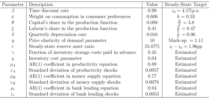
Understanding the macroeconomic effects of
working capital in the United Kingdom
∗
Emilio Fernandez-Corugedo
1, Michael McMahon
2, Stephen
Millard
3, and Lukasz Rachel
11
Bank of England
2
University of Warwick, Centre for Economic Performance (LSE) and
CAMA (ANU)
3
Bank of England and Durham Business School
May 23, 2012
Abstract
We document the behaviour of working capital over the business cycle stressing the large negative effect of the recent credit contraction on UK firms’ working capital positions. In order to understand the effects of working capital on macroeconomic variables, we build an otherwise standard flexible-price DSGE model which includes a explicit role for the components of working capital as well as a banking sector which intermediates credit. We find that financial intermediation shocks, similar to those experienced post-2007, have persistent negative effects on economic activity. Using our model as the lens through which we view the data, we find that the financial crisis in the UK can be explained by a decline in aggregate productivity and a restriction of bank lending; monetary policy acted to partly offset these shocks.
Keywords: Working capital; business cycle model; spreads; financial crisis.
JEL Codes: E30; E51; E52.
∗The views expressed in this paper are those of the authors, and not necessarily those of the Bank
of England. The authors wish to thank the editor, Wouter den Haan, and the anonymous referees for suggestions which substantially improved the paper. We are also very grateful to Kevin Lee, Katharine Neiss, Simon Price and seminar participants at the Bank of England, Reserve Bank of Australia, the Workshop on ‘Finance, Credit and Output Fluctuations’ at the University of Nottingham and the Royal Economic Society Annual Conference 2011 for their many helpful comments. An earlier version of this research was published on April 18 2011 as Bank of England working paper 422. McMahon thanks Ilona Serwicka for excellent research assistance. Any errors and omissions remain the fault of the authors. Correspondence to [email protected].
1
Introduction
Firms spend much time managing their working capital. This is especially true in re-cessions, when the flows of cash are particularly uncertain, and perhaps even more so in banking crises when the availability of credit is affected even more than usual. However, most macroeconomic models do not consider an explicit role for either working capital or a banking sector. While there are a few existing papers that incorporate a working capital channel, and there is a growing literature that models a banking sector, there is little evidence on the important interactions of the two. This paper is an attempt to address this gap in the literature in both an empirical and theoretical way.
Working capital is defined as the difference between current assets (which are firms’ resources in cash or readily convertible into cash such as inventories1) and current
liabil-ities (i.e., firms’ cash requirements). However it is the economic concept, rather than the accounting definition, that matters for firms; firms have a funding gap between when they pay the costs of inputs to production (such as labour) and when they receive the revenue from the sales of output which typically comes much later.2 As such, working capital represents operating liquidity available to firms and having the right amount of working capital at the right time is therefore crucial for the efficient operation of businesses.
Decisions about working capital are driven mainly by liquidity considerations. The financial crisis affecting the world economy that started during the summer of 2007 put a premium on liquidity not only on the financial sector but also on the corporate sector. In particular, the ‘credit crunch’ put pressure on firms’ working capital positions. This was a concern to policymakers at the time. For example, the Bank of England’s Monetary Policy Committee noted in their December 2008 meeting that:
‘the non-banks [. . . ] were apparently concerned about their own liquidity positions and were holding more short-term cash [. . . ]. Such concerns partly reflected the deterioration in the macro-economic outlook, which was likely to put pressure on corporate cash flows and the availability of working capital.’ It is clear from this that working capital problems may affect the supply side of the economy. For example, problems in the financial sector may increase the cost of raising liquidity for firms, leading to an increase in their overall costs. Uncertainty about receiving payments for goods/services rendered, together with difficulties obtaining trade credit insurance, may lead some firms to delay production (possibly affecting employment) until the uncertainty dissipates. Moreover, working capital difficulties may result in
1Also referred to, mainly in the UK, as stocks.
2In fact, as we will see in Section 2, the same aggregate amount of working capital in terms of the accounting definition can be driven by very different underlying behaviours. For example, during the recent financial crisis in the UK, inventories were initially very high and net cash very low but then later the level of inventories was very low while net cash had been built up.
firm insolvencies and, thus, capital scrapping and higher unemployment. According to these supply-side arguments, weak working capital positions are likely to result in lower employment and output but higher inflation.
The purpose of our paper is to understand how the responses of key macroeconomic variables such as investment, inventories, employment, output and inflation to economic shocks are affected by the need for firms to raise working capital. To this end, this paper makes three contributions. The first is to document the behaviour of the components of working capital in the United Kingdom both on average over business cycles, as well as over the recent financial crisis. This is important as there is scant evidence on this potentially important transmission channel of economic shocks. This analysis provides a motivation for both our paper and further research on the topic. It also provides us with a series of stylised facts against which to assess the suitability of the model.
Second, we develop a flexible price dynamic stochastic general equilibrium (DSGE) model that introduces an explicit role for working capital components. We then use this model to investigate the effects of financial shocks to bank lending, in addition to those to productivity and monetary policy. While no paper has modelled all of the components of working capital in a general equilibrium framework, various papers have successfully introduced individual components in general equilibrium models. As it is our intention to try to keep our model as parsimonious as possible, we adopt the approach to each component that is reasonably simple and tractable. In particular, we choose to motivate firms’ and households’ use of money via cash in advance constraints; we model inventories as an input into the production function; and we apply a simple, exogenous concept of trade credit. We shall judge whether our assumptions are reasonable by the extent to which the model matches the stylised facts in the empirical data.
Our model takes Christiano and Eichenbaum’s (1995) framework as a starting point (Christiano and Eichenbaum (1992) and Fuerst (1992) are related models), adding a banking sector which is subject to reserve ratio shocks and inventories in production. In the model, firms have to finance their labour and inventories input in advance of production (and hence of sales and revenue) which means that they have to borrow from financial intermediaries. This model differs from others in the literature in that our working capital constraint considers inventory behaviour, a key element of working capital and a major input to the production process, as well as a reduced form concept of trade credit. Our model incorporates this extended constraint with a stylised banking sector. This banking sector generates spreads between borrowing and lending rates of interest, and allows us to use our model to examine how an increase in spreads, such as that induced by financial disruption in 2007 and 2008, might affect the economy via its effect on working capital. It is the combination of these shocks from the banking sector, together with the firms’ working capital constraint, that is important for the results in
this paper.3
We feel it is important to include inventories for three reasons: (i) inventories are a key component of firms working capital positions, (ii) inventories in general account for a large proportion of the volatility of GDP (McMahon (2012) shows that the variance of inventories and associated covariance terms account for almost half of the volatility of US GDP growth), and (iii) inventories initially built up and then collapsed sharply in the financial crisis and so they provide an important test of our model’s performance. While there are numerous alternative approaches to modelling inventories (such as, for example, the stock-out avoidance or (s, S) decision rules) which may be more appropriate for the analysis of trends in inventory behaviour, their solution approaches involve complex numerical techniques which would limit the extent to which we can additionally consider other components of working capital. We therefore proceed using the commonly used assumption that inventories are used as inputs to production.
Our final contribution is to use the model to investigate the effect of different shocks in driving the behaviour of the UK macroeconomy during the financial crisis; this exercise is similar in spirit to the exercise carried out by Ohanian (2010). We find, using our model as the lens through which we view the financial crisis, that the initial falls in GDP, employment and inventories in 2008 are brought about by productivity and bank lending shocks; while monetary policy acts to mitigate the response of output, employment and inventories, it cannot fully offset the effects. The assumption of fully flexible prices seems to be rejected but we nonetheless conclude that disruptions to the supply of credit have had large and persistent effects on the real economy through this working capital channel. The rest of the paper is structured as follows. In Section 2, we examine the business cycle behaviour of working capital and its components in UK data and, in particular, look at how working capital has been affected by the recent financial crisis. Section 3 discusses the model, its calibration and its performance at matching the main stylised facts of the data. This section also establishes that firms’ requirement to raise working capital does not markedly affect the response of the economy to standard productivity shocks. Section 4 discusses the model’s predictions for how financial and monetary shocks affect the real economy via working capital. In Section 5 we present the estimation of the shocks that drive the financial crisis and Section 6 concludes.
3Christiano, Motto, and Rostagno (2010) present a larger model that similarly includes the interaction of working capital and financial shocks. While they do not model each component of working capital, they do include, in addition to a ‘bank funding cost channel’, a standard ‘financial accelerator channel’. And Jermann and Quadrini (2012) study an environment in which the amount of debt that is available to finance firm operations, including paying the wage bill, has real affects and drives a wedge between the marginal product of labour and the wage rate. Khan and Thomas (2011) investigate financial shocks which are propagated through the aggregate capital stock (rather than labour demand) as a result of collateralized borrowing and partial capital irreversibility.
2
The empirical behaviour of working capital
In this section, we look at the cyclicality and persistence of the constituent parts of working capital in UK data with a special focus on their behaviour in the recent financial crisis. Knowledge of these stylised facts is important to motivate the importance of our modelling contribution, and will hopefully also stimulate further work on the topic. These facts will also help us assess whether our model has the right implications for the variables in which we are most interested.
2.1
Stylised facts since 1987
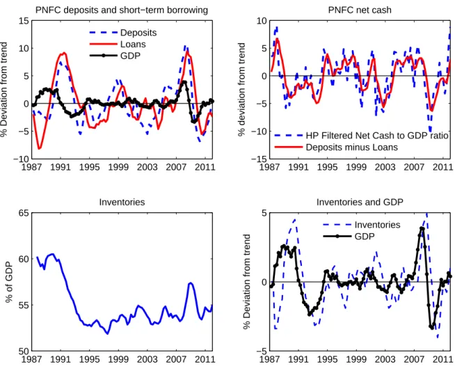
First we look at measures of corporate liquidity: deposits, loans and the difference be-tween the two (net cash holdings). The top left panel of Figure 1 looks at smoothed, detrended deposits and short-term borrowing of private non-financial companies (PNFCs) in the United Kingdom and compares these with detrended real GDP.4 We report the
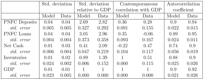
moments of these data, along with standard errors and the model equivalent statistics, in the first three panels of Table 3 in section 3.5. PNFCs’ deposits and short-term borrow-ing are around three times more volatile than GDP. Deposits are mildly procyclical while short-term borrowing is acyclical (the contemporaneous correlation of deposits with GDP is 0.28 and the equivalent figure for short-term borrowing is -0.06). And both deposits and borrowing are persistent; the AR(1) coefficients are 0.94 and 0.95, respectively.5 The top right panel of Figure 1 suggests that the ratio of net cash is also persistent, with an AR(1) coefficient of 0.69. We plot two series for net cash: the difference between detrended PNFCs’ deposits and detrended short-term borrowing (the definition we will use across data and model) and net cash as the HP-filtered net cash to GDP ratio; both series are highly correlated as can be seen in the Figure.
The bottom left panel of Figure 1 shows that the ratio of inventories to GDP trended downward somewhat until the late 1990s, since when it has been stable. Elder and Tsoukalas (2006) attributed this trend, which actually began in the mid 1970s when the inventory to GDP ratio was around 0.75, to the introduction of lean production techniques in which firms minimised on inventory levels by increasing the rate at which they received inputs and sent out their product, and by taking advantage of the improvements in information and communications technology (ICT) to manage their production on a “just-in-time” basis. Our model is not designed to analyse any of these issues and,
4Short-term borrowing includes sterling and other currency loans from both domestic and foreign banks. These data were detrended using a Hodrick-Prescott (HP) filter with the smoothing parameter set to 1600. PNFC deposits and loans are both then smoothed using the double-exponential smoothing approach; GDP is unsmoothed. Given that the end of our sample includes the financial crisis, we verified our detrending by using a Baxter-King band-pass filter at frequencies between six and 32 quarters. As the main conclusions were insensitive to the chosen approach, we use the HP filter.
1987 1991 1995 1999 2003 2007 2011 −10 −5 0 5 10 15
% Deviation from trend
PNFC deposits and short−term borrowing Deposits Loans GDP 1987 1991 1995 1999 2003 2007 2011 −15 −10 −5 0 5 10
% deviation from trend
PNFC net cash
HP Filtered Net Cash to GDP ratio Deposits minus Loans
1987 1991 1995 1999 2003 2007 2011 50 55 60 65 % of GDP Inventories 1987 1991 1995 1999 2003 2007 2011 −5 0 5
% Deviation from trend
Inventories and GDP Inventories GDP
Figure 1: Working Capital Behaviour in the United Kingdom Notes: The top left figure plots the cyclical movements in smoothed deposits and smoothed short-term borrowing of private non-financial companies (PNFCs) in the United Kingdom and compares these with (unsmoothed) cyclical movements in real GDP. We estimate the cyclical components using a Hodrick-Prescott (HP) filter and smooth the financial series with a double-exponential smoothing technique. The top right and bottom left panels show, respectively, two measures of the level of PNFCs’ net cash holdings and the level of inventories expressed as a percentage of GDP. The bottom right panel shows HP-filtered inventory holdings and HP-filtered GDP.
instead, takes the desired inventory-GDP ratio as given.
The bottom right panel of Figure 1 shows that detrended inventories are strongly procyclical; the contemporaneous correlation with GDP is 0.51 and it appears to be particularly high in downturns. Inventories are more volatile than GDP, with the ratio of standard deviations equal to 1.39, and are persistent, with an autocorrelation coefficient of 0.9. These stylised facts are summarised in the second last panel of Table 3.
2.2
The response of working capital to the recent financial shock
The recent financial crisis has put the working capital positions of many firms under pressure. Some firms were affected directly through tighter financing conditions, quantity
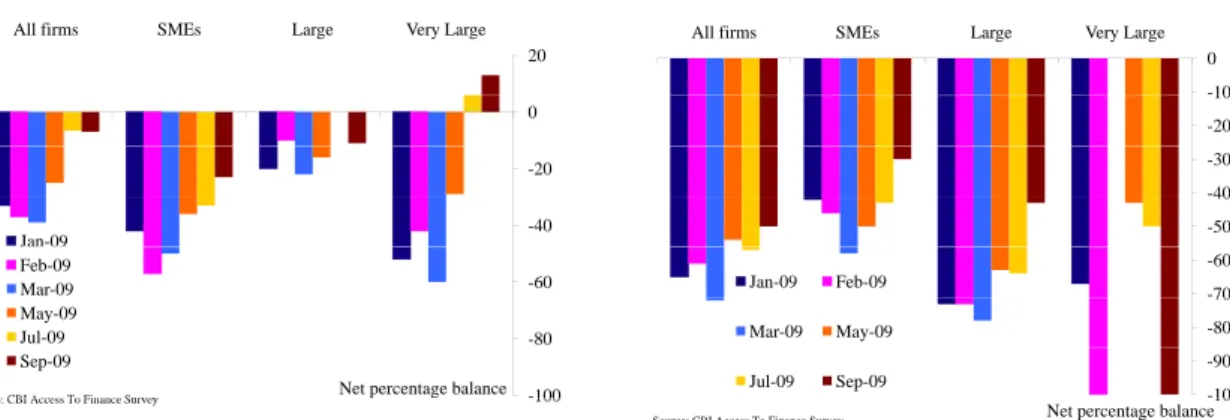
constraints on borrowing or through lower profits, and others were affected indirectly through the supply chain. A British Chambers of Commerce (BCC) survey suggests that firms’ cash flow positions, in both manufacturing and service sector, were particularly weak in late 2008/early 2009. A separate survey conducted by the Confederation of British Industry, and shown in the left panel of Figure 2, suggests that tighter financing conditions were affecting the ability of UK firms to raise working capital during the first half of 2009, even for very large firms.
But how has this affected their deposits and borrowing and their holdings of invento-ries? Looking again at Figure 1, firms’ deposits and short-term borrowing both peaked in 2008 Q1. As the economy slowed over 2008, especially in the second half of 2008 after the collapse of Lehman Brothers in September 2008, firms saw falling demand and falling revenues. Firms cut back on their borrowing but as deposits were falling faster than borrowing, their net cash positions deteriorated. In the immediate aftermath of the financial crisis, their inventory holdings rose (likely reflecting the lack of demand).
Firms reacted to these developments in two ways. Firms had responded to the tighter credit conditions by increasing their deposit holdings; as shown in Figure 1, firms net cash position began to improve as firms held more and more cash despite the continued weakness of demand conditions. It was evidence of these developments from the Bank’s regional agents that prompted the concern of the MPC in December 2008. This concern is reflected in the quote we used in the introduction. The bottom right panel of Figure 1 also shows that firms dramatically reduced inventory holdings and unwound the earlier build-up; in fact, between Q3 2008 and Q1 2010 the UK economy reduced inventory holdings in every quarter.
Ideally, we would also carefully examine the impact on trade credit which is a third major component of working capital. While the right panel of Figure 2 suggests that the availability of trade credit insurance was greatly reduced in 2009 (a development which would almost certainly have led to a reduction in trade credit), we unfortunately do not have timely data with which to assess the cyclical movements in trade credit.6
3
Our working capital model
3.1
Model overview and timing assumptions
Our model takes as its starting point the model of Christiano and Eichenbaum (1995) and adds input inventories as well as a stylised banking sector that is set up such that it
gen-6The data that is available is only at annual frequency and they are calculated from individual firms’ balance sheets in the Bureau van Dijk dataset; as an illustration, we find that net trade credit is procyclical with a contemporaneous correlation with GDP of 0.42. The interested reader is referred to the earlier working paper version of this paper, Fernandez-Corugedo, McMahon, Millard, and Rachel (2011), for more details.
Figure 2: Evidence of Working Capital Stress during the financial crisis Availability of working capital finance
All firms SMEs Large Very Large 20 0 -20 -40 Jan-09 -60 Ja 09 Feb-09 Mar-09 -80 May-09 Jul-09 -100 Sep-09
Net percentage balance
Source: CBI Access To Finance Survey 100 Source: CBI Access To Finance Survey
Availability of trade credit insurance
All firms SMEs Large Very Large
-10 0 -20 10 -40 -30 -50 40 -70 -60 Jan-09 Feb-09 -80 70 Mar-09 May-09 -100 -90 Jul-09 Sep-09 100 Net percentage balance
Source: CBI Access To Finance Survey
Notes: Both figures plot the Net Percentage Balance of answers, by firm size, to specific questions in the Confederation of British Industry (CBI) Access to Finance survey. The Net Percentage Balance shows the percentage of respondents reporting that “Availability of finance for working capital” (left panel) or “Availability of trade credit insurance” (right panel) had improved in the last 3 months minus the percentage reporting a deterioration; a negative number implies that the balance of respondents reported a deterioration. We plot a selection of survey results from the first nine months of 2009; data up to 2011 are not available as the CBI discontinued the survey.
erates positive spreads between lending and deposit rates. The model is a flexible-price, monetary model consisting of five agents: the central bank, households, firms, input in-ventory suppliers and financial intermediaries (banks). The central bank follows a money supply rule which we impose exogenously. We have a utility-maximising representative household which supplies labour to firms and consumes final goods. Firms maximise profits by selling final goods, which are produced using labour, capital and input inven-tories, to consumers. The firm’s input inventories are provided by materials suppliers who extend only limited trade credit which increases the working capital required by firms. Firms borrow from banks for working capital purposes; the banks simply channel the savings of consumers to firms subject to exogenous (stochastic) reserve requirements. Although they act as a veil, we will show that they can have important implications for output and the monetary transmission mechanism; we show that negative financial shocks can reduce real activity such as GDP and employment, but also highlight that there is a role for monetary policy in offsetting such shocks.
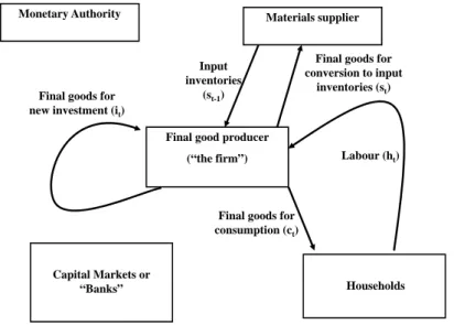
Figure 3 shows the real (top panel) and financial (bottom panel) flows in our model and is useful to highlight the differences between our model and that of Christiano and Eichenbaum (1995) (CE). Like the CE model, the firm in our model hires labour from households which is subject to a working capital constraint for which it borrows from the financial intermediary sector; in both models, the firm then sells final output to households (as consumption goods) as well as reinvesting some of the final output as new capital.
Our first major departure from the CE framework is that we also introduce materials (input) inventories as a factor of production and we require that the costs associated with these input inventories be partly financed with working capital (the remainder is provided on trade credit).
The second distinction is in the operation of our banking sector. While both models contain financial intermediaries, the banks in our model are subject to (stochastic) reserve requirements; this means that the size of their lending activity, expressed as a percentage of their overall balance sheet, varies over time. The financial structure also generates a positive spread between lending and deposit rates which is key in terms of generating a role for monetary policy in reducing the effects of banking shocks in our model. As in the CE model, the household is the ultimate owner of all firms and receives profits from each sector at the end of each period.
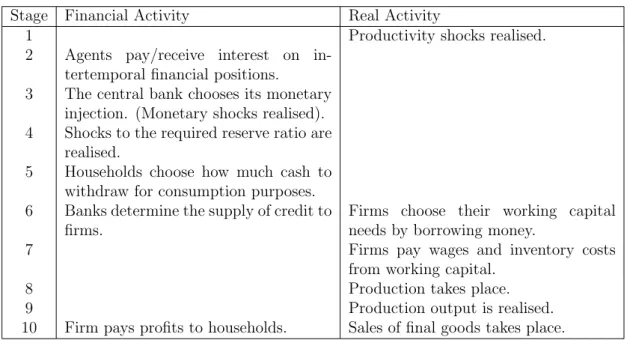
Each agent’s behaviour is discussed in greater detail below, but in Table 1 we first summarise the timing of the main financial and real activities within each time period.
Table 1: Timing of events in our model
Stage Financial Activity Real Activity
1 Productivity shocks realised.
2 Agents pay/receive interest on
in-tertemporal financial positions.
3 The central bank chooses its monetary
injection. (Monetary shocks realised).
4 Shocks to the required reserve ratio are
realised.
5 Households choose how much cash to
withdraw for consumption purposes.
6 Banks determine the supply of credit to
firms.
Firms choose their working capital needs by borrowing money.
7 Firms pay wages and inventory costs
from working capital.
8 Production takes place.
9 Production output is realised.
10 Firm pays profits to households. Sales of final goods takes place.
At the start of the period the productivity shock is realised and agents, who enter the period with holdings of liquid and illiquid assets, pay or receive interest on their intertemporal financial positions as soon as financial markets open.
The central bank chooses its monetary injection knowing the productivity shock but not knowing the banks’ desired reserve ratio and hence the loan supply.7 We assume that households are subject to a cash-in-advance constraint which requires them to have cash to pay for their consumption needs. The household, therefore, chooses how much cash
7If the central bank could observe the financial shock ahead of injecting reserves, then it would be able to completely undo its effect.
Figure 3: Real and Financial Flows in the Working Capital Model Real Flows in the Model
Final good producer (“the firm”)
Materials supplier
Households Final goods for
new investment (it)
Final goods for
consumption (ct)
Input inventories
(st-1)
Labour (ht)
Final goods for conversion to input
inventories (st)
Capital Markets or “Banks” Monetary Authority
Financial Flows in the Model
Final good producer (“the firm”)
Materials supplier
Households Payment for
final goods Payment for materials transformation service (part trade credit)
Wages Capital Markets or “Banks” Deposits / Withdrawals Lending Profits Profits Profits Repayment with Interest Monetary Authority Monetary Injection
to withdraw for consumption purposes. Banks determine the optimal supply of credit to firms who borrow for their working capital needs; credit supply depends on the shock to the desired reserve ratio which is the last shock to be realised.
The focus then shifts to the production phase of the period. Firms hire labour and pay for the cash-in-advance share of their input inventory costs using the working capital that they borrowed from the banks. Production takes place and the firm can then choose the price of output which will determine sales; the remainder of realised production output is used for investment or converted into input inventories by materials suppliers to use in the
next period. Once the final goods are sold to consumers and input inventory suppliers, the firm determines its end-of-period deposits and profits are paid into households’ bank accounts.
3.2
Model agents
3.2.1 Firms
We assume that firms, owned by households, are monopolistic competitors and have some price-setting power. Modelling this as a production aggregator version of the Dixit and Stiglitz (1977) model, each individual firm, j, faces a demand curve for their product given by Φj,t = Pj,t Pt −η Φt (1)
where Φj denotes sales for firm j, Pj is the price set by firm j, η captures the own-price
elasticity of demand and Φ denotes aggregate demand (sales). We assume a continuum of firms of measure one so that, in equilibrium, Φj = Φ and Pj =P ∀j.
The firm produces output using three inputs; capital, labour, and inventories. The capital stock is owned by the firm (which makes investment decisions each period). Firms hire labour from the households, and use input inventories from materials suppliers. The production technology for firm j is:
yj,t =kθj,t−1(Athj,t)ξs
1−θ−ξ
j,t−1 (2)
where yj is gross output of firm j, kj is firm j’s end-of-period capital stock, hj is the
labour input, sj is firm j’s end-of-period holding of inventories and A is a technology
shock common to all firms.
It may seem strange that we model inventories as a factor of production; inventories chosen in period t−1 are used in period t as inputs to production in a manner that fol-lows, among others, Kydland and Prescott (1982), Christiano (1988) and Ramey (1989). Inventories differ from the capital stock in that inventories depreciate fully after their use (once an inventory is used as an input in production, the good is used up) whereas capital depreciates only slowly over time. As we discuss in Appendix A.1, such an approach is an accepted way of generating the positive correlation between inventories and GDP that we observe in the data without requiring the use of more complicated solution techniques. The inventories in our model can be thought of as either input (materials and supplies) or work-in-progress inventories; we have, as a result of this modelling choice, ignored final good inventories but we feel content to do this as input manufacturing inventories account for 2.5 times as much volatility as final good manufacturing inventories in the
UK data (Tsoukalas 2005).8
As in CE we impose a working capital constraint on firms such that they must pay households for the wages and a fraction, γ, of the materials inventory costs in advance of sales revenue being realised. We treat the remainder of inventory costs, (1−γ), as a form of trade credit. Firms need working capital loans, Lt, to finance this funding
gap. Our working capital constraint is simply an extension of the standard working capital constraint to include inventory costs and also allow for a degree of trade credit in inventory costs; typical working capital constraints require only that the firm pay the wage bill in advance.
We require that firms fully repay their loans out of their current deposits; this is a kind of cash-in-advance constraint on the firms debt repayment.9 As the firm needs financial
resources to meet these obligations, firmj faces two financial constraints:
Fj,t−1 ≥(1 +il,t−1)Lj,t−1 (3) Fj,t−1−(1 +il,t−1)Lj,t−1+Lj,t =Wthj,t+γPtχsj,t−1 (4)
where Fj denotes firm j’s bank deposits, il denotes the interest rate paid on bank loans,
W is the nominal wage, hj denotes firm j’s labour input and P χ denotes the cost of
tranforming one unit of final good into one unit of input inventory.
The first of these constraints ensures that firms hold some of the cash they receive from sales in the form of deposits with which to repay short-term working capital borrow-ing. We prevent the firm from building up liquid assets by assuming that the firm pays out all profits except the future costs of repaying their current period borrowing. This means equation (3) will bind in our equilibrium and, as a result, the second constraint reduces to ensure that the firm borrows (Lt) to exactly cover all input costs that must be
paid in advance. Preventing firms from building up large enough liquid assets to ensure that the constraint that they face does not bind is a trick used in many macroeconomic models with financing constraints; see, for example, Carlstrom and Fuerst (1997) in which entrepreneurs are assumed to be impatient in order to ensure the borrowing constraint remains binding, and Bernanke, Gertler, and Gilchrist (1999) in which there is an exoge-nous probability of death of the entrepreneur which results in the consumption of all net worth. As we will show later our model overstates the procyclicality of loans and this
8Iacoviello, Schiantarelli, and Schuh (2011) present a model of both output and input inventories. 9In the existing literature there are three popular ways of ensuring that firms hold cash: money in the production function, liquidity considerations as in Kiyotaki and Moore (2008) and a cash in advance constraint. The practice of introducing money in the production function is a reduced form approach to impose a role for money and to capture the ‘economic efficiency’ of a monetary, rather than a barter, economy (Sinai and Stokes 1972) or the cost saving ‘bookkeeping entries’ purchased from the financial industry (King and Plosser 1984). Kiyotaki and Moore (2008) endogenously generate a role for money in a model where liquidity, the only special characteristic of money, is important due to the difficulty in reselling some assets to fund new investment opportunities.
simplification may capture why; in the data, firms can use retained profits (which are high when GDP is high) to reduce the amount of borrowing they need to do, while we rule out this possibility in the model.
Of gross output produced in periodt, the firm sells some to consumers, some is used as investment to build the capital stock and the remainder is converted into input inventories for use in the production of period t+ 1 output. The overall flow of goods for firm j is:
yj,t = Φj,t+ (kj,t−(1−δ)kj,t−1) +sj,t (5)
The firms set their price and choose production inputs, together with loans and de-posits, so as to maximise the (utility-weighted) present discounted value of the flow of dividends they pay to households. For firm j the problem is:
Maximise {kj,t,hj,t,sj,t,Pj,t,Lj,t,Fj,t} E0 " ∞ X t=0 βt Ptct (Πfj,t) # (6)
whereβ is the households’ time discount rate, ct is real household consumption (c1t is the
marginal utility of the household) and Πfj,t is the nominal profits of firm j at time t. The firm’s profit flow is given by inflows of sales revenue less wages, interest on loans and inventory storage costs. Hence, the money it will have available out of which to pay dividends will equal the sum of profits, net new borrowing, and deposits. The remainder will equal the firms’ end-of-period deposit holdings. Hence for firm j:
Fj,t+ Πfj,t =Pj,tΦj,t−Wthj,t−Ptχsj,t−1−il,t−1Lj,t−1+ (Lj,t−Lj,t−1) +Fj,t−1 (7)
The overall maximisation problem for firm j is to choose production inputs, prices and borrowing and cash so as to maximise (6) subject to (1), (3), (4), (5) and (7). The resulting first order conditions, together with the assumption that there is a continuum of firms of measure one, yields the following aggregate optimality conditions:
1 ct =βEt 1 ct+1 θktθ−1(At+1ht+1)ξs1 −θ−ξ t + 1−δ (8) 1 ct =βEt 1 ct+1 (1−θ−ξ)kθt(At+1ht+1)ξs −θ−ξ t − χ Pt+1 (1 +γil,t+1) η η−1 (9) ξkθt−1Aξthtξ−1s1t−−1θ−ξη−1 η = Wt Pt (1 +il,t) (10) Ft= (1 +il,t)(Wtht+γPtχst−1) (11) st =ktθ−1(Atht)ξst1−−1θ−ξ−(kt−(1−δ)kt−1)−Φt (12) Lt=Wtht+γPtχst−1 (13) Πft =PtΦt−Ft−(1−γ)Ptχst−1 (14)
Equation (8) sets the expected user cost of capital equal to the real interest rate at the optimum; equation (9) is the analogous optimality relation for inventories in which the expected user cost of inventories is set equal to the real interest rate. Equation (10) is a labour demand curve that says the firm is more willing to hire labour the lower is the real wage and the loan rate (since it must borrow the money to pay wages). Equation (11) defines how much the firm needs to deposit in order to pay off its loan during the following period. Equation (12) states that total output is either sold, invested or shipped to materials suppliers to be used in production in the following period. Equation (13) simply defines how much the firm needs to borrow. Finally, equation (14) simply defines the dividend paid by the firm to the consumer at the end of the period.
3.2.2 Materials suppliers
We consider a very simple structure for the sector that provides input inventories. The materials firms, owned by households, act like distribution agents for goods to be allocated among the final good firms. These suppliers do not use any labour or capital but are simply able to convert final output into input inventory for use by final good firms in the following period. For these distribution (or transformation) services, the sector is paid a fee per unit which we denote byPtχ.10 Precisely, in periodtthe materials sector takesst
goods from the final goods sector and agrees to convert these into input inventories for delivery in periodt+ 1. The profit from this activity is paid to households at the end of the period. Profits are given by:
Πst =Ptχst−1 (15)
Not all input inventories services can be purchased using trade credit. Instead, the materials suppliers will offer a share (1−γ) of the costs on trade credit but the remainder must be payed before delivery and production of the inputs; this means that the firm must borrowγPtχst−1 up front which implies that input inventories add to the working capital
requirements in our model relative to standard models with working capital constraints.
3.2.3 Financial institutions and the central bank
We now outline the behaviour of the banks in our model which, as mentioned above, is the other main departure from more standard working capital models.11 However,
10The absence of a cost means that the materials firms would like to supply infinite transformation services which would drive the price of transformation,Ptχ, to zero. To prevent this, we setχ as a
pa-rameter of the model meaning the price of turning final goods into input inventory is always proportional to the price level.
11The reader interested in more details about the intra-period flows and balance sheet of the banking sector can refer to the appendix of the earlier working paper version of this paper (Fernandez-Corugedo, McMahon, Millard, and Rachel (2011)).
in common with other working capital models, the financial sector in our model is kept relatively simple. The banks in our model act simply to channel the savings of households to the corporate sector as loans. As in CE, these loans are specifically for the purpose of working capital: they bridge the funding gap between the payment for inputs into production, and the arrival of the payments for the produced output.
We build on the financial intermediaries modelled in Dhar and Millard (2000) and, as the banking sector, per se, is not our interest in this work, we do not explicitly model the profit maximising behaviour of banks. In fact, we assume there is sufficient competition for zero profits to be made and model banks’ desired reserve-asset ratio as being determined exogenously. We allow this desired ratio, a key determinant to the amount of loans made by the banking sector, to be hit by random shocks (which we label loan supply shocks).12 The banking sector is, in our model, a source of shocks rather
than a channel of independent propagation and our interest is seeing how these financial shocks affect macroeconomic variables through firms working capital requirements.
Overall, the financial system can be summarised by the following three equations, which we address in turn:
Rt+Lt=Dt+Bt+Ft (16) Πbt =il,t−1Lt−1−id,t−1Dt−1 = 0 (17) Lt= (1−rt)((1 +id,t−1)Dt−1+Xt+Bt−1) rt (18) Equation (16) represents the balance sheet equilibrium of the banking sector, (17) rep-resents the banks’ profits which are zero each period and equation (18) reprep-resents the lending decision of banks which is determined by the desired reserve ratio (rt) in each
period.
The bank balance sheet contains three different types of deposit account that comprise banks liabilities; liquid deposit accounts held by firms (Ft−1) and by households (Bt−1),
as well as illiquid (savings) accounts held by households (Dt−1).13 The most important
distinction concerns the liquidity of an account which relates to the timing in the model. Illiquid account deposits, once made, cannot be accessed again until the start of the following period while liquid accounts can be accessed at any time. We assume that the Bank pays deposit interest (id,t) only on illiquid accounts. This distinction is similar
to the treatment by banks of savings accounts (time deposit in the US) and current
12In our model, the fact that money never leaks out of the banking system implies that there is a zero probability of a bank run; given this, banks would never wish to hold reserves. However, we feel that imposing an exogenous reserve asset ratio captures the fact that, in reality, banks do hold reserves to ensure that they can meet withdrawals and the level of reserves they hold can change for what looks like purely exogenous reasons.
13Materials suppliers do not carry positive balances between periods although they would, within a period, have positive balances before they transfer all balances to the household.
(checking) accounts.14
The beginning of period t bank balance sheet is:
Banking sector balance sheet at the start of period t
Assets Liabilities
Rt−1 Dt−1
Lt−1 Bt−1
Ft−1
As well as deposit balances from the end of period t−1, firms enter the period with outstanding loansLt−1 (an asset for the bank). Finally, financial institutions, in addition
to having loan assets (Lt−1), also hold reserves (Rt−1) at the central bank. This is a credit
economy in which the financial sector will determine the size of credit flows through the economy. Nonetheless, high-powered money - reserves - is created only by the monetary authority through monetary injections. There will be many transfers across accounts during the period but at the end of period t the bank balance sheet will be dictated by equation (16).
The monetary authority can affect the total size of the bank balance sheet via a mon-etary injection, Xt, which we assume goes straight to household deposit accounts and
so boosts the level of reserves. Technically, this is equivalent to a government transfer to households financed by printing money and is fairly standard in the “limited partic-ipation” literature. Through monetary injections, the central bank has complete con-trol over the level of reserves in this economy; we shall therefore model total reserves,
Rt =Rt−1+Xt, as being subject to central bank control and model money supply shocks
as shocks to total reserves.
Households receive interest on their illiquid depositsid,t−1and the firms pay interest on
their loansil,t−1.15 Bank profits, given by the difference between the financial inflows and
financial outflows, are denoted Πbt−1 =il,t−1Lt−1−id,t−1Dt−1. We impose that competition
in the banking sector is sufficient to yield zero profits which suggests that il,t−1Lt−1 = id,t−1Dt−1 as in equation (17).
Consumers who are subject to a cash-in-advance constraint for consumption pur-chases, must decide how much of their resources, (1 +id,t−1)Dt−1+Bt−1, they wish to to
leave as illiquid deposits in the bank. The trade-off is the following; illiquid deposits will yield an interest return but cannot be used for consumption in that period. The con-sumer will choose to transfer Tt (which could be negative) to their liquid assets (which,
14In reality, liquid (checking) accounts may pay some interest but the key for our analysis is that there is a positive spread between the interest paid on illiquid (savings) deposits and liquid (checking) deposits by these accounts.
by definition, are available for use at anytime but do not yield an interest return. This re-balancing of the household savings portfolio only affects the liabilities side of the balance sheet.
Banks use some of their liabilities to make loans to firms for working capital. That is, the banking sector determines the amount of lending to provide which affects total working capital and thus the level of production. As no money leaks out of the banking sector in this credit economy, the loans made become deposits in the banking sector and so we get a multiplier effect. The balance sheet of the banking sector expands:
Banking sector balance sheet in the middle of period t
Assets Liabilities
Rt−1+Xt (1 +id,t−1)Dt−1+Xt−Tt
Lt Bt−1+Tt
Lt
Rather than explicitly model an optimal lending decision, we assume that financial institutions have a desired reserve asset ratio of rt. We model this reserve ratio as a
stochastic process.16 Hence, their desired lending is given by:
Lt= (1−rt)((1 +id,t−1)Dt−1+Xt−Tt+Bt−1+Tt+Lt), (19)
which re-writes as (18).
The banking sector will expand credit such that the reserve asset ratio meets its target. If rt = 1, then there is no lending and banks act simply to store ‘money’; as
rt →0, Lt → ∞ and there is no limit to the amount of lending the financial system will
provide. Firms borrow working capital loans, Lt, to finance their funding gap and the
loan interest rate adjusts to clear the credit market.
After the lending decision is made, access to deposit accounts is closed off; all remain-ing money flows in the economy are made via liquid accounts. Wages are paid into the household liquid account (Bt) out of which nominal consumption is financed. There are
flows between firms for trade credit as well as the final good firm receives sales revenue. At the end of the period, dividends are paid into households liquid accounts. The bank’s balance sheet at the beginning of the next period is given by an analogous balance sheet to the beginning of period t and is captured by equation (16).
16This represents an end of period reserve asset ratio as no further credit is created; there are simply redistributions between accounts.
3.2.4 Households
The household is fairly standard and maximises the present discounted value of utility derived from consumption of final goods and from leisure. For simplicity, we assume that preferences over consumption and leisure are natural logarithmic with (constant) weights
ψ and (1−ψ) respectively: Maximise {ct,ht,Tt} E0 " ∞ X t=0 βt((1−ψ) ln(ct) +ψln(1−ht)) # (20)
As we described above, the main financial decision of the household is to choose the level of its illiquid assets (Dt) by choosing an amount to transfer Tt to its liquid assets;
they choose ((1 +id,t−1)Dt−1+Xt−Tt) as illiquid assets and (Bt−1+Tt) as liquid assets.
These decisions are made once all uncertainty is resolved.
Once this decision is made, they choose how much to consume and how much to work (for which they earn wages). As there is no interest paid on illiquid deposits, and as there is no uncertainty left to resolve, households will transfer just enough resources such that they then consume all of their liquid resources available to them:17
Ptct=Bt−1+Tt+Wtht (21)
where P denotes the price level, c denotes consumption, W denotes the nominal wage and h denotes total hours worked.
The household’s bank balances at the beginning of period t+ 1 will be given by:
Dt =(1 +id,t−1)Dt−1+Xt−Tt (22) Bt =Π f t + Π b t + Π s t (23)
The household chooses ct, ht and Tt to maximise (20) subject to (21), (22) and (23).
The first order conditions imply: 1 Ptct =β(1 +id,t)Et 1 Pt+1ct+1 (24) ht = 1− ψPtct (1−ψ)Wt (25)
Equation (24) is the standard consumption Euler equation that links expected growth in consumption to the real interest rate. Equation (25) is a labour supply curve that says the consumer is more willing to supply labour the higher is the real wage and the marginal
17After they make their consumption choices, they will receive the profit flows from firms, banks, and materials suppliers into their illiquid account; these resources could not have been consumed but they make their transfer decision knowing that such wealth was going to arrive.
utility of consumption (the lower is consumption itself). Equations (21) to (25) represent five optimal conditions for the household.
3.3
Equilibrium and exogenous variables
We solve the 16 derived conditions for a maximum18 together with the goods market
clearing condition, c= Φ, conditional on A, R,and r, for the 17 unknownsc, k, h, s, Φ,
P,W, Πf, Πs, D, B, M, L, F,R, i
d and il.
We log-linearise the model around its steady state; in Appendix B we discuss the implications of this linearisation as well as out assumptions used for solving the model. We have three variables in our model representing our exogenous, stochastic variables;19 we assume that these exogenous variables all follow AR(1) processes:
ˆ At =ρAAˆt−1+εA,t (26) ˆ rt =ρrrˆt−1+εr,t (27) ˆ Rt =ρRRˆt−1+εR,t (28)
Where ‘hats’ denote log deviation from steady state. Equation (26) represents the process for productivity shocks, (27) is the process for bank lending shocks and (28) captures the dynamics of money supply shocks caused by the monetary authority; it is worth highlighting that a positive shock to rt represents a higher reserve ratio and a
decline in bank lending (a negative bank lending shock).
3.4
Calibration
As a first exercise, we calibrate our model to quarterly UK data over the period 1976 Q1 to 2011 Q4 in order to ascertain how well it fits the stylised facts presented earlier as well as examine how the working capital channel affects the response of the economy to a productivity shock.
The main calibration parameters are laid out in Table 2. We set β= 0.99 implying a steady state deposit rate of 0.0101 per quarter (4.1% per annum). We normalise hours worked to equal 0.33 in steady state, implying a value for ψ of 0.606. We set capital’s share in the production function, θ, to 0.098 so as to imply a capital to gross output ratio of 3.8, the average in UK data over the calibration period. Setting ξ to 0.41 then implies a stock to gross output ratio of 0.47, equal to its average value in UK data. We set the (quarterly) depreciation rate, δ, to 0.016 so as to imply an investment to gross
18These are (8) - (14), (15), (16) - (18), and (21) - (25).
19In Fernandez-Corugedo, McMahon, Millard, and Rachel (2011) we also allowed the amount of trade credit, governed byγ, to vary as a trade credit shock. However, this variable was similar to a bank credit shock and without good data to allow us to identify it, we have dropped it from consideration in this version of the paper.
output ratio of 0.06, the average in UK data. While some of these figures may seem low for quarterly data, it is worth noting that our model and calibration implies that gross output is more than double GDP. This means targeting gross output ratios effectively reduces the target ratio by about half; for example, the capital-GDP ratio would be 7.6 in our model while the equivalent ratio in the data is 7.8, where in both cases we use the definition of GDP (or value-added output) from our model which is the sum of consumption, business investment and inventory investment.
Table 2: Model Calibration
Parameter Description Value Steady-State Target
β Time discount rate 0.99 id= 4.1%p.a.
ψ Weight on consumption in consumer preferences 0.606 h= 0.33
θ Capital’s share in the production function 0.098 KY = 3.8
ξ Labour’s share in the production function 0.41 S
Y = 0.47
δ Quarterly depreciation rate 0.016 YI = 0.06
η Price elasticity of demand parameter 10 Mark-up = 1.11
r Steady-state reserve asset ratio 55.87% il−id= 1.96pp
γ Fraction of inventory storage costs paid in advance 0.45 Estimated
χ Inventory cost parameter 0.04 Estimated
ρA AR(1) coefficient in productivity equation 0.89 Estimated
εA Standard deviation of productivity shocks 0.0057 Estimated
ρR AR(1) coefficient in money supply equation 0.77 Estimated
εR Standard deviation of money supply shocks 0.0078 Estimated
ρr AR(1) coefficient in bank lending equation 0.94 Estimated
εr Standard deviation of bank lending shocks 0.0053 Estimated
Notes: This table shows the values of parameters used in our calibration as well as empirical data we targeted. The estimated parameters are discussed in further detail in Section 5 below.
On the nominal side, we normalise the price level to equal unity and set η equal to 10 implying a mark-up of 1.11. We target a steady-state spread of the loan rate over the deposit rate equal to 1.96 percentage points: the average spread of nominal PNFC’s loan rates over the Bank of England’s policy rate over the calibration period.20 To achieve this
target we must set a reserve asset ratio, r, equal to 55.87% in steady state. While this is large relative to what might be expected to prevail in the banking sector, it is worth noting that our banks are greatly simplified and hold a much less varied array of assets and liabilities, and since we are more concerned with hitting the correct average spread, we are willing to overlook the discrepancy in this ratio.
The most difficult parameters to calibrate, given the lack of good quality trade credit data (and the absence of trade credit data at the quarterly frequency) were the terms related to the materials suppliers. To get around this issue, we estimated a version of our model in which, in addition to the shock parameters, we also recover estimates for χ
20The average spread of PNFC Loan interest rates over PNFC Deposit interest rates, available from 1999 Q1, is 2 percentage points.
of 0.04 and a value for steady state γ of 0.45. We therefore set the parameters at these estimated values and it is worth pointing out that the main estimation we use below is one in which the parameters χ and γ are calibrated at these levels. In Table 2 we report the estimated shock parameters; the main estimation from which these are derived is explained in greater detail in Section 5.
Our calibration has the following implications for some key, non-targeted GDP ratios in the data. In our model, the ratio of consumption to private sector value-added output is 86% and of investment to private sector value-added output is 14% in line with their values in UK data for our sample. Our model implies a labour share equal to 67% compared with 69% in the data. Finally, in the model corporates’ gross money holdings are equal to 69% of private sector value-added, gross debt holdings are equal to 68% of private sector value-added and net money holdings are equal to 1.4% of private sector value-added. These values compare with PNFCs’ deposits being equal to 66% of nominal GDP in 2009 Q4, PNFCs’ short-term lending being equal to 59% of nominal GDP in 2009 Q4 and net cash being equal to 7% of nominal GDP in 2009 Q4.
3.5
Stylised facts in the model
We now report the stylised facts generated by our model using the parameter values reported in Table 2 and compare the statistics to the empirical equivalents reported in Section 2. Table 3 shows that using the estimated shock processes generally does well in matching the main stylised facts of the data. The main exception is net cash. The model cannot match the volatility of the actual data (it misses by a factor of about five) and the contemporaneous correlation with GDP is the wrong sign. This is because the contemporaneous correlation between loans and GDP is too high in the model (the actual data suggest no significant correlation between loans and GDP) which means that overall net cash falls in the model when there is an increase in GDP (compared to an increase in the data). We discussed above how our assumption that firms cannot build up liquid assets to reduce their reliance on bank lending may be a reason for this. Nonetheless, we are satisfied that our model is a close enough proxy for the data in which we are most interested.
3.6
How do working capital considerations affect the response
of the economy to shocks?
We now consider how the working capital constraint and other assumptions that we have made affect the economy’s dynamics in response to a typical productivity shock. To this end, we compare the responses of the real variables in our working capital model (WK model, presented above) with a comparison RBC model in which there is no working
Table 3: Stylised facts
Std. deviation Std. deviation Contemporaneous Autocorrelation
relative to GDP correlation with GDP coefficient
Model Data Model Data Model Data Model Data
PNFC Deposits 0.04 0.04 2.69 2.82 0.36 0.28 0.9 0.94 std. error 0.005 0.005 0.327 0.292 0.091 0.155 0.022 0.015 PNFC Loans 0.04 0.04 3.05 2.96 0.35 -0.06 0.89 0.95 std. error 0.004 0.004 0.373 0.358 0.093 0.167 0.024 0.011 Net Cash 0.01 0.03 0.41 2.09 -0.22 0.47 0.74 0.9 std. error 0.006 0.004 0.047 0.219 0.104 0.117 0.056 0.019 Inventories 0.01 0.02 0.89 1.39 1 0.51 0.88 0.9 std. error 0.024 0.002 0.006 0.152 0.000 0.115 0.025 0.026 GDP 0.01 0.01 1 1 1 1 0.9 0.92 std. error 0.023 0.005 0.000 0.000 0.000 0.000 0.021 0.026
Notes: The moments were computed using GMM and the standard errors with the delta method; see, for example, Hevia (2008). See den Haan and Levin (1997) for a discussion of using GMM to estimate standard errors. All series are detrended using a Hodrick-Prescott filter with the smoothing parameter of 1600 except the Net Cash series which is the difference between PNFC deposits and PNFC loans. PNFC deposits and loans are additionally smoothed using a double-exponential smoothing approach.
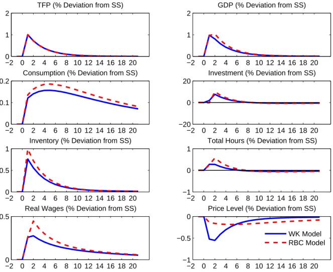
capital constraint but in which there are inventories; calibration and other assumptions are otherwise the same and the comparator model is presented in the appendix. Figure 4 presents the impulse responses to a 1% productivity shock; they show that the responses are not substantially altered by the presence of a working capital constraint, though the need to raise working capital acts to dampen the response of hours, inventories, investment and output to the shock, while at the same time amplifying the price response. On impact, a positive innovation to productivity raises the marginal product of the factors of production and as a result output rises. To take advantage of the higher marginal productivity, firms demand more inventories, labour and, after a one-period delay, capital. Real wage rises in response to the increased demand for labour. Both real consumption and labour supply increase. The response of consumption is much smaller than that of output but much more persistent; households smooth consumption in response to the shock.21
As this is a pure positive supply-side shock, the price level falls, but the extent of the fall in the price level is crucially dependent on the presence of a working capital constraint for the firms. We can see why by considering the money demand equation in the two economies. For the economy with a working capital constraint we can write the money
21An interesting corollary to the models main results is that both models generate a hump-shaped response of consumption to the TFP shock. This persistence is not driven by assumed ‘consumption habits’ but rather by the inclusion of inventories and the working capital constraint in the model. As it is not germane to the main point of this paper, we have left the discussion for future work.
market equilibrium equation, where supply of funds equals demand for funds, as:
Rt =
r
1−r(Wtht+γPtχst−1) (29)
That is, money demand (RHS) depends on components of nominal income. For the economy without a working capital constraint we can write the money market equilibrium equation as:
Rt=Ptct (30)
That is, money demand depends on nominal consumption. Since consumers try to smooth through changes in their income, nominal income and its components rise by more than consumption and this means that the price level must fall by more in the economy in which money demand depends on nominal income (namely, our working capital model). We shall see later that the model’s predictions about the magnitude of price movements are larger than we find in the data.
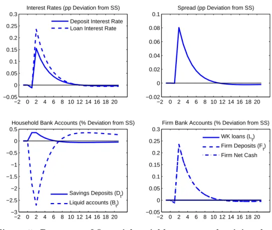
Figure 5 shows the responses of financial variables to the productivity shock for our working capital model alone. Consumers’ illiquid deposits rise when the productivity shock hits; anticipating higher (real) labour income, households save to smooth their consumption by leaving more of their wealth in the form of illiquid savings. Although firms want to borrow more given the positive supply shock, loans to the corporate sector remain unchanged since we assume banks’ desired reserve-asset ratio remains unchanged and there is no increase in reserves. In order to ensure that this happens, the loan rate must rise. Given that illiquid deposits increase and loans stay fixed, the banks’ zero-profit condition implies that the deposit interest rate must rise by less than the loan rate so the spread between the two rises. As the spread rises, firms increase their net cash holdings. The positive comovement between spreads and productivity actually poses a challenge for our model in terms of matching the precise movements of the spread data.
4
The effects of financial shocks
In this section we focus on our main interest which is the effects of shocks in the financial sector. We start by looking at the predictions of the model for how real and financial variables respond to shocks to banking lending, before checking to what extent monetary policy can affect the economy and have real effects. We then briefly discuss how trade credit, if we modelled it as a stochastic process, would affect the economy. Finally, we use the model as the lens through which we view recent developments and can assess both the extent to which different shocks appear to have played an important role, and also the broad fit of our model to the empirical data.
−2 0 2 4 6 8 10 12 14 16 18 20 0 1 2 TFP (% Deviation from SS) −2 0 2 4 6 8 10 12 14 16 18 20 0 1 2 GDP (% Deviation from SS) −2 0 2 4 6 8 10 12 14 16 18 20 0 0.1 0.2
Consumption (% Deviation from SS)
−2 0 2 4 6 8 10 12 14 16 18 20 −20
0 20
Investment (% Deviation from SS)
−2 0 2 4 6 8 10 12 14 16 18 20 0
0.5 1
Inventory (% Deviation from SS)
−2 0 2 4 6 8 10 12 14 16 18 20 −1
0 1
Total Hours (% Deviation from SS)
−2 0 2 4 6 8 10 12 14 16 18 20 0
0.5
Real Wages (% Deviation from SS)
−2 0 2 4 6 8 10 12 14 16 18 20 −1
−0.5 0
Price Level (% Deviation from SS)
WK Model RBC Model
Figure 4: Response of real variables to a productivity shock Notes: This figure plots the response of the real variables in the model to a 1% shock to productivity which evolves according to equation (26). The responses are shown for both the baseline working capital model (“WK model”) as well for a model in which there is no working capital constraint and hence no meaningful role for banks to provide loans to the firm (“RBC model”).
4.1
Banking sector shock
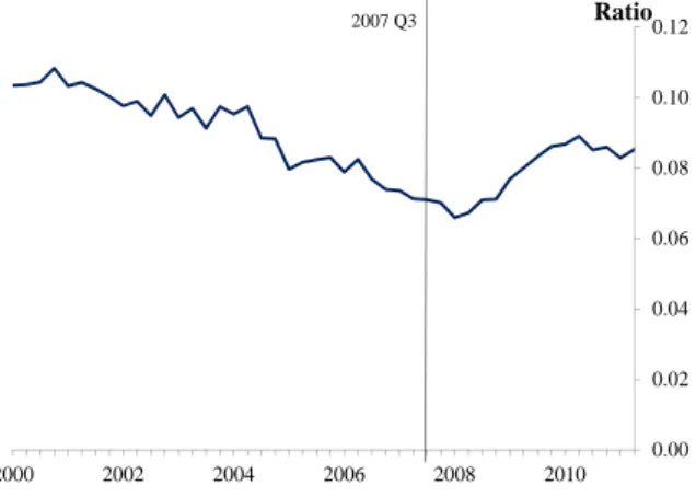
As discussed earlier, within our model we think of a financial shock as a shock resulting in a higher holding of reserves by banks (and a lower level of lending) for a given level of bank deposits. This is consistent with what happened in the UK banking sector after the run on Northern Rock in September 2007 and then the failure of Lehman Brothers in 2008. As confidence among the banks fell, their costs of obtaining wholesale funds rose and this led to an increase in the ratio of bank reserves to bank lending whereas previously this ratio had been trending down, as shown in Figure 6.22
22Unfortunately, the series for M4 lending adjusted for intermediate other financial corporations (OFCs) only goes back to 1998; the ratio of notes and coin in circulation to M4 lending has been on a downward trend since about 1970, although the trend was interrupted between about 1992 and 2004 where the ratio was basically flat.
−2 0 2 4 6 8 10 12 14 16 18 20 −0.05 0 0.05 0.1 0.15 0.2 0.25 0.3
Interest Rates (pp Deviation from SS)
Deposit Interest Rate Loan Interest Rate
−2 0 2 4 6 8 10 12 14 16 18 20 −0.02 0 0.02 0.04 0.06 0.08 0.1
Spread (pp Deviation from SS)
−2 0 2 4 6 8 10 12 14 16 18 20 −3 −2.5 −2 −1.5 −1 −0.5 0 0.5
Household Bank Accounts (% Deviation from SS)
Savings Deposits (D t) Liquid accounts (B t) −2 0 2 4 6 8 10 12 14 16 18 20 −0.05 0 0.05 0.1 0.15 0.2 0.25 0.3
Firm Bank Accounts (% Deviation from SS)
WK loans (L t) Firm Deposits (F
t) Firm Net Cash
Figure 5: Response of financial variables to a productivity shock Notes: This figure plots the response of the financial variables in the model to a 1% shock to productivity which evolves according to equation (26). The responses are shown for the baseline working capital model.
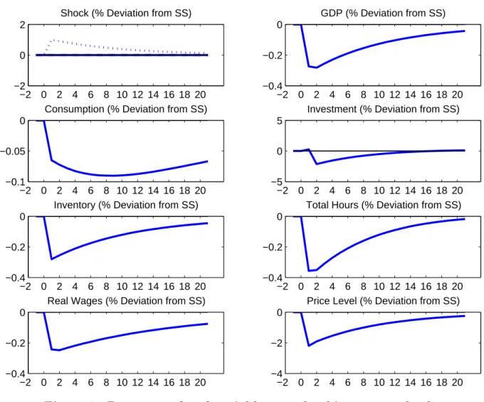
Figures 7 and 8 consider the effects of a 1% shock (+0.56 pp) to the banks’ desired reserve asset ratio on financial and non-financial variables, respectively. In our model the banks’ lending decision is simple: they lend out a proportion, 1−rt of their liabilities.
So the most obvious effect of the negative bank lending shock, i.e. a positive shock to rt
is to cause a sharp contraction in lending. This shock effectively works as a withdrawal of money available to the private sector. Given available reserves Rand monetary policy injection X, banks now hoard more money and so less is available for everyone else. In this way our model replicates the squeeze on firms’ lending in the aftermath of the credit crisis. The interest rate at which firms are able to borrow goes up (+0.27 pp). In this sense this shock is similar to a contractionary monetary shock. Consequently, the price level falls. While both firm loans and deposits decline, loans actually fall by more than deposits; net cash rises. At first sight, this seems to differ from the behaviour of net cash in the data. As shown in Figure 1, deposits initially declined more quickly than short-term loans. Net cash turned positive in 2009 as loans continued to fall and deposits levelled off.
On the real side, the higher borrowing costs feed through to higher input costs. Specif-ically, it is now more costly for a firm to finance its labour input and inventories, and so
Figure 6: Ratio of notes and coins in circulation to PNFCs short-term bor-rowing 0.00 0.02 0.04 0.06 0.08 0.10 0.12 2000 2002 2004 2006 2008 2010 Ratio 2007 Q3
Notes: This figure plots ratio of notes and coin in circulation to M4 lending.
demand for these inputs falls. Consequently, firms produce less and output falls. Firms demand less labour and so the real wage falls. Consumers face a loss of labour and profit income and to smooth the impact of the shock they save more via illiquid assets and lower liquid assets in the first period, but these revert to mean over the following periods. The interest paid on deposits falls.
The responses to the financial intermediation shock discussed here show that even though prices are fully flexible in our model, a disruption to the supply of credit has large and persistent effects on the real economy. In particular, output, consumption and investment fall (lowering the capital stock persistently) and real wages remain weak for a long time. This may help to explain large and persistent effects of financial crises found in numerous studies.23 Overall, the model’s predictions of a contraction in lending followed by marked falls in output, hours worked and investment together with sharp decumulation of inventories in the model closely resembles what happened during the recent crisis and suggests that the working capital channel was important in explaining the dynamics of the recent downturn in the United Kingdom. We return to a quantitative evaluation of this issue Section 5.
4.2
Monetary policy shock
In a model with no working capital considerations and with flexible prices, a monetary injection (by which we mean X, a government transfer of cash to consumers) will have no effect on real variables. However, given that firms have to borrow to finance working capital purchases, monetary policy shocks will, even in a world of flexible prices, have effects since they will affect the quantity and cost of the liquidity that firms require for
−2 0 2 4 6 8 10 12 14 16 18 20 −2
0 2
Shock (% Deviation from SS)
−2 0 2 4 6 8 10 12 14 16 18 20 −0.4 −0.2 0 GDP (% Deviation from SS) −2 0 2 4 6 8 10 12 14 16 18 20 −0.1 −0.05 0
Consumption (% Deviation from SS)
−2 0 2 4 6 8 10 12 14 16 18 20 −5
0 5
Investment (% Deviation from SS)
−2 0 2 4 6 8 10 12 14 16 18 20 −0.4
−0.2 0
Inventory (% Deviation from SS)
−2 0 2 4 6 8 10 12 14 16 18 20 −0.4
−0.2 0
Total Hours (% Deviation from SS)
−2 0 2 4 6 8 10 12 14 16 18 20 −0.4
−0.2 0
Real Wages (% Deviation from SS)
−2 0 2 4 6 8 10 12 14 16 18 20 −4
−2 0
Price Level (% Deviation from SS)
Figure 7: Response of real variables to a banking sector shock Notes: This figure plots the response of the real variables in our working capital model to a 1% shock to banks’ desired reserves which evolves according to equation (27).
their working capital. Figure 9 considers the effect of a 1% monetary injection in our working capital model. Given that the monetary injection leads to a fall in the spread, it becomes cheaper for firms to finance the inputs of production. Firms increase output by increasing their use of inventories and hours worked. Since the shock is expected to persist, firms also want to increase their capital; as a result investment rises and the capital stock is persistently higher. Finally, households increase their consumption though consumption smoothing implies the increase is small and highly persistent. Nominal wages and prices both rise, but by less than the rise in reserves (because some of the nominal shock leaks into real variables) and with nominal wages rising more than prices. The response of nominal variables is shown in Figure 10. The monetary injection leads to a rise in the deposits of consumers (both liquid and illiquid deposits) and firms as well as a rise in loans. Importantly, firms’ net cash holdings fall; the shock leads to a narrowing in the spread between loan and deposit rates with the implication that firms
−2 0 2 4 6 8 10 12 14 16 18 20 0 0.1 0.2 0.3 0.4 0.5
Interest Rates (pp Deviation from SS)
Deposit Interest Rate Loan Interest Rate
−2 0 2 4 6 8 10 12 14 16 18 20 0 0.05 0.1 0.15 0.2
Spread (pp Deviation from SS)
−2 0 2 4 6 8 10 12 14 16 18 20 −2.5 −2 −1.5 −1 −0.5 0 0.5
Household Bank Accounts (% Deviation from SS)
Savings Deposits (D t) Liquid accounts (B t) −2 0 2 4 6 8 10 12 14 16 18 20 −3 −2.5 −2 −1.5 −1 −0.5 0 0.5
Firm Bank Accounts (% Deviation from SS)
WK loans (L t) Firm Deposits (F
t) Firm Net Cash
Figure 8: Response of financial variables to a banking sector shock Notes: This figure plots the response of the financial variables in our working capital model to a 1% shock to banks’ desired reserves which evolves according to equation (27).
need to hold lower deposits to pay back a given level of loans.
Importantly, these responses make it clear that the reaction of policymakers to devel-opments in the economy will be key. In the model, the central bank has full control over the banking sector balance sheet and, ceteris paribus, the overall amount of broad money in the economy; it therefore can, to an extent, offset the adverse effects of a financial shock. Indeed, if, as in C´urdia and Woodford (2009), one assumes that a central bank follows a traditional Taylor rule but also responds to the increase in spreads by injecting money to ensure that interest rates fall, then the effect of the shock on output is smaller than in our benchmark case (where reserves were held unchanged) and the effect on the price level is reversed: inflation rises following the banking shock.