MODEL FOR DYNAMIC SHEAR MODULUS AND DAMPING

M

ODEL FOR

D

YNAMIC

S

HEAR

M

ODULUS AND

D

AMPING

FOR

G

RANULAR

S

OILS

By Dominic Assimaki,

Eduardo Kausel,

Fellow, ASCE,

and Andrew Whittle,

Member, ASCE

ABSTRACT: This paper presents a simple four-parameter model that can represent the shear modulus factors and damping coefficients for a granular soil subjected to horizontal shear stresses imposed by vertically prop-agating shear waves. The input parameters are functions of the confining pressure and density and have been derived from a generalized effective stress soil model referred to as MIT-S1. The predicted shear moduli and damping factors are in excellent agreement with high quality resonant column test data on remolded sands and confining pressures ranging from 30 kPa to 1.8 MPa. The proposed model has been implemented in a frequency domain computer code. By simulating the variations in stiffness and damping with confining pressure, the proposed model provides a more realistic simulation of ground amplification that does not filter out high fre-quency components of the base excitation.

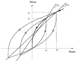
FIG. 1. Loading-Unloading at Different Strain Amplitudes INTRODUCTION

It is now standard practice in seismic engineering to take into consideration the nonlinear behavior of soils undergoing time-varying deformations caused by earthquakes. While it is in principle possible to perform true incremental analyses in which the soil properties are adjusted according to the load path and instantaneous levels of strain, this is seldom done in practice. Instead, in the most widely used approach, approxi-mate linear solutions are obtained using an iterative scheme originally proposed by Seed and Idriss (1970). In this method, the soil properties are chosen in each iteration in accordance with some characteristic measure of strain computed in the previous iteration. While the linear iterative solution may not provide an exact solution to the nonlinear soil dynamics prob-lem at hand, it often produces acceptable results for engineer-ing purposes (Constantopoulos et al. 1973). SHAKE (Schnabel et al. 1972) is perhaps the best known and most widely used computer program using this type of iterative linear algorithm. Much progress has also been made recently in laboratory experiments attempting to simulate the in situ conditions that might exist in deep soil deposits (Laird and Stokoe 1993). Soil samples subjected in these tests to confining pressures as high as 5 MPa have revealed patterns of nonlinear behavior that, while qualitatively similar to the response under lower confin-ing pressures, exhibited less degradation of shear modulus with strain (i.e., remained nearly elastic). The damping due to hysteresis was correspondingly smaller. Testing at higher con-fining pressures has proved a difficult task. Thus, it is desirable to develop an analytical model, such as SHAKE, that can sup-plement the experimental data and can be used in computer models of wave propagation in soils.

NONLINEAR SOIL BEHAVIOR

Once shearing strains exceed about 10⫺5

(referred to as the linear threshold), the stress-strain behavior of soils becomes increasingly nonlinear, and there is no unique way of defining

1

Grad. Res. Fellow, Massachusetts Inst. of Technol., Cambridge, MA 02139.

2

Prof. of Civ. and Envir. Engrg., Massachusetts Inst. of Technol., Cam-bridge, MA.

3_{Assoc. Prof. of Civ. and Envir. Engrg., Massachusetts Inst. of}

Tech-nol., Cambridge, MA.

Note. Discussion open until March 1, 2001. To extend the closing date one month, a written request must be filed with the ASCE Manager of Journals. The manuscript for this paper was submitted for review and possible publication on June 10, 1999. This paper is part of the Journal

of Geotechnical and Geoenvironmental Engineering, Vol. 126, No. 10,

October, 2000.䉷ASCE, ISSN 1090-0241/00/0010-0859–0869/$8.00⫹

$.50 per page. Paper No. 21230.

shear modulus or damping. Therefore, any approach to char-acterize the soil for analyses of cyclic loading of larger inten-sity must account for the level of cyclic strain excursions.

When ground motions consist of vertically propagating shear waves and the residual soil displacements are small, the response can often be characterized in sufficient detail by the shear modulus and the damping characteristics of the soil un-der cyclic loading conditions. It is usual practice to express the nonlinear stress-strain behavior of the soil in terms of the secant shear modulus and the damping associated with the energy dissipated in one cycle of deformation. With reference to the hysteresis loop shown in Fig. 1, the secant modulus is usually defined as the ratio between maximum stress and max-imum strain, while the damping factor is proportional to the

area ⌬E enclosed by the hysteresis loop, and corresponds to

the energy dissipated in one cycle of motion. It is readily ap-parent that each of the aforementioned properties depends on the magnitude of the strain for which the hysteresis loop is determined; thus they are functions of the maximum cyclic strain.

The simplified response illustrated in Fig. 1 can be de-scribed through a backbone curve, corresponding to first load-ing, together with a set of rules for unloading and reloadload-ing, as proposed by Masing. Rheological models of this type can be represented by a set of elastoplastic springs in parallel, with input parameters obtained by curve fitting the measured data. When opting for an equivalent linear analysis, the charac-terization of the soil consists of three parts (Fig. 2):

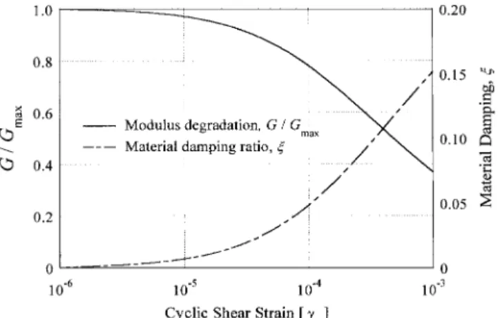
FIG. 2. Secant Modulus and Material Damping Ratio as Func-tion of Maximum Strain

• The maximum shear modulus Gmaxin the very small strain

linear region.

• The reduction curve for G/Gmax versus maximum cyclic

strain␥c(referred to as modulus degradation curve), with

G being the secant modulus.

• The fraction of hysteretic (or material) damping␰versus the maximum cyclic strain ␥c. This parameter is defined

as the area ⌬E of the hysteresis loop and normalizing it

by the ‘‘elastic’’ strain energy through the following ex-pression:

1 ⌬E

␰= 2 (1)

2␲G␥c

In the case of dry cohesionless soils, the physical origin of the variation in modulus and damping with cyclic strain, as reflected in the shapes of the curves in Fig. 2, is now well understood. Both parameters are related to the frictional be-havior at the interparticle contacts and the rearrangement of the grains during cyclic loading (Dobry et al. 1982; Ng and Dobry 1992, 1994). Therefore, even crude analytical models of particles can be used to mimic the degradation curves of

G/Gmaxand␰versus␥c, provided that they include friction and

allow for particle rearrangements.

It should be noted however that reversible behavior is as-sociated with minimal rearrangement of particle contacts and irrecoverable, plastic strains become significant only at strain levels␥cⱖ 0.1%. Therefore, for smaller cyclic strain

ampli-tudes dissipation of energy must be related to frictional be-havior at contacts.

EFFECT OF CONFINING PRESSURE ON MODULUS AND DAMPING

Cohesionless Soils

The modulus degradation and damping curves most often used for dry cohesionless soils, such as sands and gravels, are those proposed by Seed and Idriss (1970). Based on the ex-perimental data by Hardin and Drnevich (1970) and others, these standard curves are extensively used in equivalent linear analysis of earthquake excitations and machine vibrations. The approach by Seed and Idriss (1970) assumes that the G/Gmax

and␰curves are essentially the same for sands, gravels, and cohesionless silts. Their generic response curves assume that the degradation curves are independent of the cycle number considered as well as the void ratio (or relative density, sand type, and confining pressure). However, it should be noted that all the aforementioned factors do significantly affect the max-imum shear modulus Gmax.

Laboratory measurements provide evidence in support of

some of these simplifying assumptions. They show that void ratio, overconsolidation, sand type, and cycle number (Iwasaki et al. 1978; Dobry et al. 1982) do indeed have relatively small influence on the measured backbone curves. They also show that the method of sand deposition, existence of static shear stress, grain size (sands versus gravels) are also of secondary importance (Hardin 1965; Hardin and Drnevich 1972a; Tat-suoka et al. 1979; Seed et al. 1986). However, the influence of the confining pressure is significant and cannot possibly be ignored, especially when performing dynamic analyses for deep soil deposits.

A number of laboratory studies (described later) on hydro-statically consolidated sands have shown that their stress-strain response becomes more linear as the confining pressure in-creases (i.e., as␴0increases, G/Gmaxincreases and␰decreases).

[Laboratory data show minor influence of K0 on the shear

modulus degradation and damping curves (Hardin and Drne-vich 1972a).] In addition, large confining pressures lead to substantial reductions in material damping at small strain (i.e., ␰min). The reason for these effects with increasing␴0is related

to the different rates at which the small strain modulus and the shear strength of the soil increase when the pressure in-creases (Hardin and Drnevich 1972a; Seed et al. 1986; Laird and Stokoe 1993).

To illustrate this assertion, consider the hyperbolic model frequently used to represent the stress-strain behavior of soils. In this model, the backbone curve is defined in terms of two parameters, namely, the small strain shear modulus Gmax and

the shear strength␶max. The hyperbolic equation for the

back-bone curve is as follows:

␥

␶= (2)

(1/Gmax⫹␥/␶max)

Alternatively,␶= [␥/(␥r⫹ ␥)]␶max, in which␥r =␶max/Gmaxis

a reference strain (Hardin and Drnevich 1972b). Therefore, the corresponding modulus degradation curve is only a function of the reference strain, namely

G 1

= (3)

Gmax 1⫹(␥/␥r)

For an isotropically consolidated sand subjected to a pure shear loading, Coulomb’s strength law indicates that␶max=␴0

tan ␾, in which ␾is the angle of internal friction of the soil. On the other hand, the low strain shear modulus is usually approximated as Gmax = where m = 0.5⫾ 0.1, and A is

m

A␴0,

a constant. Consequently,␥r is proportional to and, as␴0 0.5

␴0 ,

increases, ␥r and G/Gmax increase, as verified by the

experi-mental data (Shibata and Soelarno 1975).

A later section presents experimental results obtained by Laird and Stokoe (1993), who determined the degradation curves of isotropically consolidated sand specimens subjected to confining pressures as high as␴0= 3.5 MPa. It will be seen

that high values of ␴0 lead to degradation curves that lie

be-yond the bands given by Seed and Idriss (1970). Hence, use of the standard curves for dynamic response analyses involv-ing cohesionless soils at very high confininvolv-ing pressures could be unconservative, as those curves might severely overestimate nonlinear effects in the soil as well as its tendency to dissipate energy.

Wet Cohesionless Soils

The degree of saturation in cohesionless soils certainly af-fects the reduction curves for shear moduli and damping at large shear strain amplitudes (i.e., ␥c ⱖ 0.1%). For smaller

strain amplitudes, soil behavior can be approximated as un-coupled (i.e., minimum volume change and pore pressure gen-eration are introduced by shearing). Therefore, it is presumed

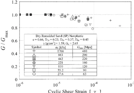
FIG. 3. Effect of Confining Pressure on Shear Modulus Degradation Curves, Measured for Dry Remolded Sand (Laird and Stokoe 1993)

that the curves for dry materials may also be applicable to saturated granular soils for shear strain amplitudes␥cⱕ0.1%,

with the response controlled by the in situ effective confining pressure

␴⬘=␴⫺u (4)

where u = in situ pore-water pressure.

Clearly, if water is not trapped between the soil particles during shear, it does not participate in the stress-strain re-sponse or in the energy dissipation in the material. In such a case, damping is completely caused by friction due to inter-actions between the particles, as if the soil was dry. It should be noted, however, that this might not apply to small strain, high frequency cyclic loads in a resonant column test. In such a case, damping values will be higher for a saturated material because of viscous effects caused by the relative movement between the solid phase and the pore water. This difference in damping between dry and saturated soil is generally not sig-nificant for low frequency dynamic phenomena such as earth-quakes, but may be relevant to high frequency vibrations such as generated by explosions and machine vibrations.

EXPERIMENTAL DATA ON COHESIONLESS SOILS To determine the dynamic properties of granular soils at significant depths, Laird and Stokoe (1993) carried out labo-ratory tests at the University of Texas at Austin. The objective of the experiments was to determine the dynamic properties of soils at significant depths for dry and saturated specimens at confining pressures up to␴0= 3.5 MPa. The results of these

tests demonstrate the effects of confining pressure on shear modulus and damping described previously.

Washed mortar sand was used to build remolded sand spec-imens. The sand is poorly graded, with a medium to fine grain size, and is classified as SP in the Unified Classification Sys-tem. For the construction of the remolded sand specimens, the undercompaction method (Ladd 1978) was used.

Resonant column (RC) and torsional shear (TS) equipment was used to investigate the dynamic characteristics of the sam-ples tested at the high confining pressures attained by the group at University of Texas at Austin (Isenhower 1979; Lodde 1982; Ni 1987; Kim 1991). The equipment is of the fixed-free type, with the bottom of the specimen fixed and torsional excitation applied at the top. RC and TS tests were

performed in a sequential series on the same specimen over a range of shearing strains from about 10⫺4

% to slightly more than 10⫺1

% by changing the frequency of the forcing function. The primary difference between the two types of tests is the excitation frequency. In the RC test, frequencies above 20 Hz are required and inertia of the specimen and drive system are needed to analyze these measurements. On the other hand, slow cyclic loading with frequencies generally below 5 Hz is prescribed in the TS tests and inertia does not enter the data analysis.

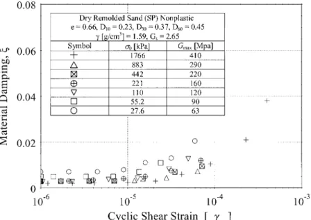
Figs. 3 and 4 show the shear modulus degradation and ma-terial damping curves for different values of confining pres-sure, respectively. The results show that the cyclic strain at the linear limit increases with the confining pressure. Figs. 5 and 6, on the other hand, show the dependence with the level of confinement of the small strain shear modulus Gmax and

ma-terial damping␰min. Clearly, materials with higher confinement

are stiffer at small values of strains.

The need to implement concisely the experimental results presented previously into a computer code for seismic ampli-fication provided the motivation for formulating a theoretical model representing the effect of confining pressure on the soil behavior under cyclic loading. This is described in the fol-lowing.

MIT-S1 MODEL FOR CLAYS AND SANDS

Pestana (1994) developed a generalized, effective stress soil model, referred to as MIT-S1, which describes the rate-inde-pendent behavior of freshly deposited and overconsolidated soils. The MIT-S1 model formulation is based on the incre-mentally linearized theory of rate-independent elastoplasticity. It retains the basic three-component structure of the MIT-E3 model (Whittle 1987) as follows:

• An elastoplastic model for normally consolidated soils with a single yield function, and nonassociated flow and hardening rules to describe the evolution of anisotropic stress-strain properties.

• Equations for the small strain nonlinearity and hysteretic stress-strain response in unload-reload cycles.

• Bounding surface plasticity for irrecoverable, anisotropic, and path-dependent behavior of overconsolidated soils. In addition, the MIT-S1 model addresses two well-known fea-tures of soil behavior:

FIG. 4. Effect of Confining Pressure on Material Damping Ratio, Measured for Dry Remolded Sand (Laird and Stokoe 1993)

FIG. 5. Variation in Maximum (Low Amplitude) Shear Modulus with Confining Pressure for Remolded Sand Samples (Laird and Stokoe 1993)

FIG. 6. Variation in Low Amplitude Material Damping Ratio with Confining Pressure for Remolded Sand Samples (Laird and Stokoe 1993)

• The yield behavior is a function of previous stress history and depends on the current mean effective stress and den-sity.

• Dense sands and heavily overconsolidated clays exhibit dilative behavior during shearing, while normally consol-idated clays experience primarily contractive behavior. Provided that modulus degradation and damping for 1D wave-propagation problems involve relatively small strain ampli-tudes (i.e., plastic components of deformation can be ignored), a reduced form of the MIT-S1 model can be used to model the behavior of granular materials under cyclic shear and con-stant effective stress. The goal is to develop, on a theoretical basis, the effect of confining pressure on the shear degradation curves and the material damping. The model is then used in the simulation of 1D amplification effects in a deep soil de-posit. A brief description of the MIT-S1 input parameters re-quired for 1D analysis is first presented, followed by a deri-vation of analytical expressions for the shear modulus degradation and damping ratio curves. The following para-graphs use the notation introduced by Pestana (1994). Elastic Components

Most generalized soil models assume that the elastic bulk modulus is given by a power law function of the mean effec-tive stress, while the shear modulus is obtained by assuming a constant Poisson’s ratio␮⬘. The resulting elastic formulation is found to be nonconservative (i.e., generates or dissipates energy during a closed stress path [e.g., Houlsby (1985)]. Con-servative elastic formulations for granular soils as well as clays have been recently proposed (Loret and Luong 1982; Houlsby 1985; Lade and Nelson 1987). In these cases, the resulting elastic bulk and shear moduli are complex functions of the shear stress (or stress ratio) and the mean effective stress.

In the MIT-S1 model, there is no region of true linear elastic behavior. However, the response immediately after a load re-versal is controlled by the small elastic moduli (Kmaxand Gmax)

defined as follows:

1 /6 1 / 3

Kmax 1⫹e Kmax ␶ ␴⬘

= Cb

冉 冊冋 冉 冊 册 冉 冊

pa e 2Gmax ␴⬘ pa

2Gmax 1⫺2␮⬘0

= 3

冉 冊

Kmax 1⫹␮⬘0

where ␴⬘ = ␴⬘(1v ⫹ 2 K )/30 = mean effective stress; K0

= lateral stress coefficient; = effective overbur-(=␴⬘h 0/␴⬘v0) ␴⬘v

den pressure; pa = atmospheric pressure; Cb = material

con-stant;␮⬘0= small strain Poisson’s ratio (observed immediately after a load reversal); and␶= shear stress level. In principal, this ratio can be determined from the effective stress path mea-sured during 1D unloading in laboratory triaxial tests (⌬εv <

0; ⌬εh = 0), where ␮⬘0 = (⌬␴⬘/⌬␴⬘)/(1v h ⫹ ⌬␴⬘/⌬␴⬘),v h and

is the measured effective stress path gradient after ⌬␴⬘/⌬␴⬘v h

reversal. Eq. (5) and (6) provide an incrementally conservative elastic formulation, written in terms of the tangent moduli and explicitly including the effect of the current void ratio e in soil stiffness.

Hysteretic Behavior

The description of nonlinear behavior during unloading and reloading is also described by separate components for shear and volumetric response.

In modeling the response due to vertically propagating shear waves, only nonlinear behavior during shear is required for 1D problems. The perfectly hysteretic response is based on the incremental, isotropic relations between effective stress and elastic strain rates. For a load cycle in stress space, the

per-fectly hysteretic model describes a closed symmetric hysteresis loop in the stress-strain response of the material, using a for-mulation that is piecewise continuous (i.e., the moduli vary smoothly) between stress reversal points. Appendix I sum-marizes the equations used to formulate the perfectly hysteretic MIT-S1 model for horizontal cyclic shearing of a soil that is consolidated at a constant mean effective stress level ␴⬘.

The ratio of shear to bulk moduli (for the specific case of ␴⬘= ␴⬘rev),during shearing is given by

2G 2Gmax 1

=

冉 冊

K Kmax 1⫹␻␰s

where ␰s = nondimensional distance in stress space that

de-scribes changes in the mean effective stress and stress ratio relative to conditions at the stress reversal point␶rev. For

hor-izontal shear analysis, this distance is

␶⫺␶rev

␰s=

冏 冏

␴⬘

The parameter␻ is a constant, which relates the swelling be-havior, and is selected from measurements of K0 versus OCR

during unloading. It can be determined directly from the ef-fective stress path in 1D unloading

3 (1⫹2K0 NC) 2Gmax 1⫹2K0 NC 1

␻=

冑

冋

冉

冊册

2 (1⫺K0 NC) Kmax 3 OCR1

(9)

where K0 NC= lateral stress coefficient of the normally

consol-idated deposit, and OCR1= overconsolidation ratio(␴⬘p/␴⬘v)at K0 = 1.

The stress reversal point is defined from the direction of the strain rates (Hardin and Drnevich 1972a), based on the obser-vation that the nonlinearity of the soil is most appropriately described in terms of strain history. The tangent bulk modulus during 1D unloading of a granular soil is described by

K e ␴⬘

=

冉 冊

pa (1⫹e)␳r pa

2 / 3

(1⫹␻ ␰s s) ␴⬘

␳r=

冉 冊

Cb pa

where␳r = current (tangential) slope of the hydrostatic

swell-ing curve in a log e⫺log␴⬘space diagram, and␻sdescribes

small strain nonlinearity during undrained shear. Evaluation of Model Input Parameters

The dimensionless material parameters needed to evaluate the stress-strain behavior of a soil deposit under cyclic loading using the MIT-S1 model, which can be measured directly or estimated with similar procedures for both sands and clays, are summarized below:

• K0 NC— The coefficient of lateral earth pressure at rest. It

can be directly measured from K0 consolidation or from

oedometer tests. It can also be estimated from empirical formulas [i.e., K0 NC= 1⫺sin␾⬘cs (Jaky 1948; Mesri and

Hayat 1993)], with ␾⬘cs being the friction angle at large strain conditions (critical state) in triaxial compression. For sands, this parameter is well-bounded with values = 33.6⬚⫾2.5⬚. For practical applications, and in light ␾⬘cs

of the uncertainties of the present analysis, the writers have assumed K0= K0 NCand K0 = 0.5.

• ␮⬘0— The elastic Poisson’s ratio immediately after load reversal that controls the ratio of small strain elastic mod-uli (i.e., 2Gmax/Kmax). It is determined from the initial slope

FIG. 7. Comparison of Measured Degradation Curves for Dry Remolded Sand Specimens with Proposed Model Predictions (Cb= 800;␻= 1.00;␮ⴕ0= 0.25;␻s= 2.40)

materials, the expected range of␮⬘0 is narrow with typical values ␮⬘0 = 0.20 – 0.25 for clays and freshly deposited sands.

• ␻— This parameter describes the variation of the elastic Poisson’s ratio accompanying changes in the stress ratio [(9)]. Common values of ␻ are found to be ␻ = 1.0 ⫾ 0.5 for clays and sands (Pestana 1994).

• Cb— This parameter defines the elastic bulk modulus at

small strain levels (i.e., Kmaxat stress reversal). For clean

uniform sands, average values of Cb are in the range of

800 ⫾ 100. For clays, on the other hand, the parameter

Cb decreases as the plasticity index increases. For low

plasticity clays, Pestana and Whittle (1994) reported typ-ical values of Cb= 400 – 500.

• ␻s— This parameter describes the small strain

nonlinear-ity in shear, and it is evaluated through the analysis of shear modulus degradation with strain level.

EVALUATION OF SECANT SHEAR MODULUS REDUCTION CURVES

The MIT-S1 model formulation was next specialized and used to develop analytical expressions for the secant shear modulus Gsecin terms of the maximum cyclic strain␥c, based

on the definition of the tangential shear modulus Gtan= d␶/d␥

(see Appendix I). For the evaluation of the shear modulus degradation curves, only the analytical expression of the back-bone curve (␶rev= 0; ␥rev = 0) is needed:

1 3 1 2

␥(␶) = CC C1 2␶ ⫹ C(C1⫹C )2␶ ⫹C␶ (12)

3 2

2 / 3

2e 1⫹␮⬘0 1 1 ␴⬘

C =

冉 冊

1⫹e 1⫺2␮⬘03Cb␴⬘ pa

where

␻s ␻

C =1 ; C =2

␴⬘ ␴⬘

are parameters with constant value for a given soil and level of confining pressure. The backbone curve is then defined as follows:

1 / 2 2 1 / 3 2 2

[(A⫹2C C B1 2 )C ] C(C1⫺C )2

␶(␥) = ⫹ _{1 / 2 2 1 / 3}

2CC C1 2 2C C [(A1 2 ⫹2C C B1 2 )C ]

C1⫹C2

⫺

2C C1 2 (14)

where

2 2 3 3

A = 12C C1 2␥⫹3CC C (C1 2 1⫹C )2 ⫺C(C1⫹C )2

2 2 3 3

B = (6C C )1 2 ␥ ⫹[18CC C (C1 2 1⫹C )2 ⫺6C(C1⫹C )]2 ␥

2 2 2 2

⫹10C C C1 2⫺3C (C1⫹C )2

Finally, the secant shear modulus can be written as a function of the maximum strain level

␶(␥c)

G(␥c) = (15)

␥c

This modulus differs for each level of confining pressure. Four input constants are necessary to define the backbone curve given by (15). However, given the narrow range within which three of these parameters (␮⬘,0 Cb, and ␻) can vary,

default values may be assumed for these, and only ␻s needs

to be specified for a given soil type. The proposed equations will then allow the generation of modulus degradation and damping curves, for all void ratios e and confining pressures ␴⬘. The validity of this assumption was successively verified, by conducting sensitivity analysis to investigate the effects of these parameters on the results of wave-propagation simula-tions, performed for various soil profiles.

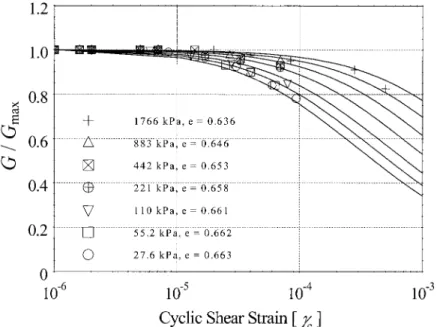
Fig. 7 shows a comparison between the shear modulus re-duction curves predicted by the proposed formulation and the experimental data presented by Laird and Stokoe (1993). Fit-ting the shear modulus degradation curve predicted by the pro-posed model for an intermediate level of mean effective stress ␴⬘ = 110 kPa, the parameter ␻s was found to be ␻s = 2.40.

Using this value, modulus degradation and damping curves were successively generated for the range of confining pres-sures of interest. Results are found to be in very good agree-ment for all tests with␴⬘= 28 – 1,800 kPa.

MATERIAL DAMPING USING MIT-S1 MODEL

Starting from the analytical expression for the backbone curve in the previous section, the theoretical value of material

FIG. 9. Comparison of Experimental Material Damping for Dry Remolded Sand Specimens and Proposed Model at Different Levels of Confining Pressure (Cb= 800;␻= 1.00;␮ⴕ0= 0.25;␻s= 2.40)

FIG. 8. Integration of Hysteresis Loop to Assess Material Damping

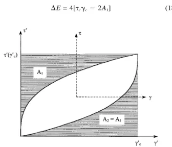
damping ␰ can also be derived as a function of maximum cyclic shear strain ␥c for different levels of mean effective

stress␴⬘,0 using (1). For this purpose, the area within the hys-teresis loop must be evaluated. It is convenient to introduce the auxiliary variables shown in Fig. 8

␶⫹␶c ␥⫹␥c

␶⬘= , ␥⬘= (16a,b)

2 2

These denote a shift of the origin of the coordinates to the lower-left reversal point and a scaling of the coordinates by a factor of 0.5. Therefore, areas measured in the transformed coordinate system are one-quarter the areas in the actual shear stress-strain coordinate system. The shaded areas above the loop can be obtained (in local coordinates) as

␶c ␶c

1 ₃ 1 ₂

A =1

冕

冕 冋

册

3 2

0 0

1 4 1 3 1 2

= CC C1 2␶c⫹ C(C1⫹C )2␶c⫹ C␶c

12 6 2 (17)

so that the area within the hysteresis loop is evaluated as

⌬E = 4[␶ ␥c c⫺2A ]1 (18)

Using (1), the resulting material damping is

1 ⌬E

␰(␥c) = 2

2␲G(␥c)␥c

2 1 ₂ 1

=

冋

冉

冊册

␲ 6 3 (19)

where G(␥c) = secant modulus associated with the strain

am-plitude␥c; and␶(␥c) is defined in (14), for␥=␥c. The results

are also summarized in Appendix I.

Fig. 9 shows very good agreement between the damping predicted by (19) at different levels of confinement(␴⬘0 = 0 – 1,766 kPa), with the experimental data on dry remolded sand specimens.

EXAMPLE OF APPLICATION

An idealized soil profile with a depth of 1,000 m and mass density varying from 2.12 ton/m3

at the surface to 2.21 ton/m3

at 1,000-m depth is subjected to an earthquake prescribed at the outcropping of rock. Two simulations are carried out in which the input motions are, respectively, the 1995 N-S JMA Kobe (Japan) and the 1989 Loma Prieta (California) accelero-grams, both scaled to a maximum acceleration of 0.05g. The soil parameters are chosen identical to the remolded sand spec-imens from Laird and Stokoe (1993). The variation of void ratio (and mass density) of the profile with depth was chosen to match the soil properties in Memphis, as reported by Abrams and Shinozuka (1997).

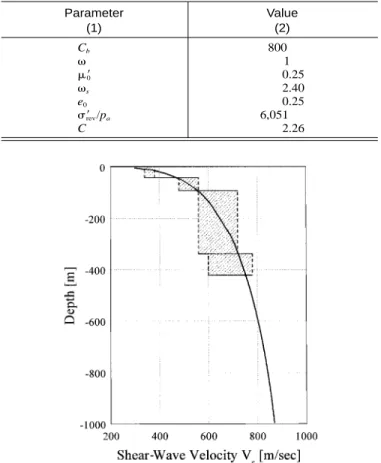
Table 1 lists the dimensionless input parameters for this model. These are used to estimate the small strain (␥= 10⫺6

) shear modulus Gmaxand to determine the modulus degradation

and damping curves. The variation of the shear-wave velocity with depth is depicted in Fig. 10, along with the reported pro-file for the Memphis area (Abrams and Shinozuka 1997). The fundamental shear-beam frequency of the soil for this profile is 0.156 Hz, and there are 20 resonant modes in the frequency range of 0 – 5 Hz.

The variation of void ratio with the mean effective stress is taken from the original formulation for the MIT-S1 model for cohesionless soils (Pestana and Whittle 1995a,b). The equa-tions needed for this calculation are summarized in Fig. 11, in which e0is the void ratio at␴⬘= 0;␴⬘r is a ‘‘reference stress’’

TABLE 1. Input Parameters for MIT-S1 Model

Parameter (1)

Value (2)

Cb 800

␻ 1

␮⬘0 0.25

␻s 2.40

e0 0.25

␴⬘rev/pa 6,051

C 2.26

FIG. 10. Soil Profile Used for 1D Soil Amplification Simulation [Measured Data from Memphis Area by Abrams and Shinozuka (1997)]

FIG. 11. Void Ratio as Function of Mean Effective Stress— MIT-S1 Compression Model

the limiting compression curve in log e-log␴⬘space. The var-iation of void ratio with confining pressure is given as follows: For first loading:

2 / 3

e 1 ␴⬘

ln

冉 冊

冉 冊

e0 2/3C pa

For the limiting compression curve regime:

1 ␴⬘

ln(e) = exp

冉 冉 冊冊

C ␴⬘r

The dynamic response of the profile at the surface is cal-culated using the computer code LAYSOL (Kausel 1992), which is based on a continuum formulation of the

wave-prop-agation problem in the frequency-wave-number domain. The soil profile is divided into 100 homogeneous layers, each 10-m thick, whose material properties are inferred from Fig. 10 (tak-ing the values at the center of the layers).

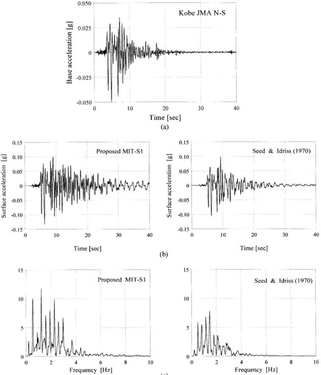
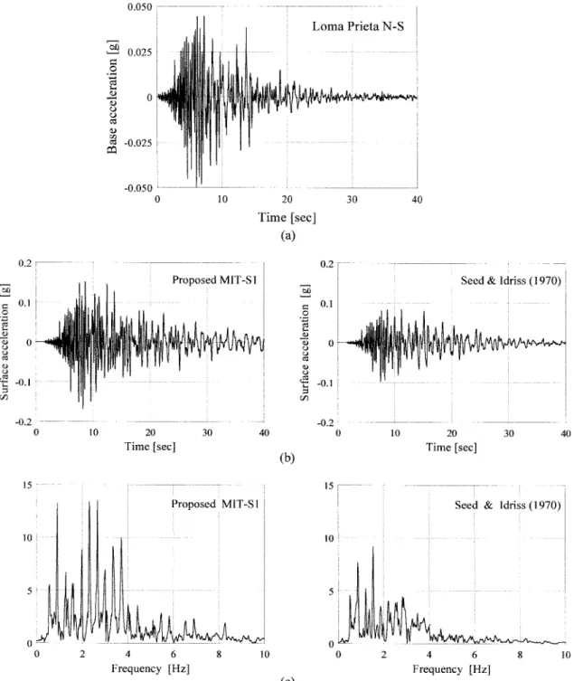
Figs. 12 and 13 present the simulation results for the Kobe and Loma-Prieta earthquakes, respectively. The time histories of these earthquakes are shown in Figs. 12(a) and 13(a). Figs. 12(b) and 13(b) exhibit the simulated motions at the free sur-face, and Figs. 12(c) and 13(c) depict the corresponding Fou-rier amplitude spectra. In Figs. 12 and 13, left-hand side shows the results obtained with the proposed pressure-dependent model formulation (reduced MIT-S1 model), and the right hand side displays those for the standard Seed-Idriss model for cohesionless soils (Seed and Idress 1970). For conven-ience, both sets of figures are drawn to the same scale. In-spection of these figures reveals several important differences between the standard and proposed models:

• The new model produces generally larger amplifications. • The high frequency components suffer much less filtering. • The duration of strong motion as well as total response

duration are longer.

All three of the above items are caused primarily by the de-crease in damping with confining pressure and, therefore, with depth.

The figures also show a characteristic 1.6-s delay in initia-tion of the response at the surface. This is consistent with the travel time of shear waves between the basal rock and the surface with an average velocity of 600 m/s (as can be inferred from the 1/6-Hz resonant frequency and the 1,000-m thick-ness). Hence, the simulations satisfy causality. In addition, the reader should observe that while the response was obtained by Fourier inversion of the frequency response functions, the time histories do not suffer from wraparound (i.e., the ‘‘dog bites tail’’ phenomenon). In other words, the coda of the response does not spill into its beginning, as could have been expected for the lightly damped system with a long natural period being considered here. These desirable characteristics are accom-plished with the ‘‘complex exponential window method’’ de-scribed by Kausel and Roe¨sset (1992).

CONCLUSIONS

This paper presented a simple four-parameter model for the dynamic shear moduli and damping characteristics of granular soils when they deform in shear only. This model is based on the MIT-S1 generalized plasticity model proposed earlier by Pestana and Whittle (1995a,b). Its four parameters can readily be measured in the laboratory, or estimated from existing data. The shear moduli and damping values predicted by the pro-posed model were found to be in excellent agreement with experimental results obtained by Laird and Stokoe (1993) over a wide range of confining pressures.

The proposed formulation takes into account the effect of confining pressure on soil parameters and hysteretic behavior and, therefore, permits proper consideration of the hysteretic characteristics of the ground with depth. As demonstrated with two simulations for a 1-km-deep site, the dependence of the dynamic moduli on confining pressure can be an important consideration in the analysis of soil deposits for earthquake effects.

The simulations indicate that, when the confining pressure is taken into account, the elasticity of the soil steadily in-creases with depth. The refinement introduced by the pressure-dependant characterization of the soil in turn alleviates signif-icantly one of the alleged shortcomings of the standard equivalent-linear model, which is that it unrealistically wipes

FIG. 12. Simulation of Wave Propagation in Deep Soil Deposit for Kobe Earthquake: (a) Input Motion; (b) Surface Response; (c) Fourier Spectra

out the high frequency components of motion when used for moderately deep to very deep soil profiles.

APPENDIX I. SHEAR MODULUS DEGRADATION AND MATERIAL DAMPING CURVES FROM 1D, PERFECTLY HYSTERETIC FORMULATIONS USED IN MIT-S1

Dimensionless Distance Measure (in Stress Space)

␶⫺␶rev

␰s=

冏 冏

␴⬘

where␶and␶rev= current stress and the stress at the reversal

point, respectively. For the definition of the backbone curve ␶rev= 0.

Definition of Tangential Elastic Moduli

K e ␴⬘

=

冉 冊

pa (1⫹e)␳r pa

2 / 3

1⫹␻ ␰s s) ␴⬘

where␳r=

冉 冊

Cb pa

2G 2Gmax 1

=

冉 冊

K Kmax 1⫹␻␰s

2Gmax 1⫺2␮⬘0

where = 3

冉 冊

Kmax 1⫹␮⬘0

where Cband␮⬘0= elastic parameters; and␻and␻s= material

FIG. 13. Simulation of Wave Propagation in Deep Soil Deposit for Loma-Prieta Earthquake: (a) Input Motion; (b) Surface Response; (c) Fourier Spectra

Definition of Backbone Curve-Secant Shear Modulus

1 / 2 2 1 / 3 2 2

[(A⫹2C C B1 2 )C ] C(C1⫺C )2

␶(␥) = ⫹ _{1 / 2 2 1 / 3}

2CC C1 2 2C C [(A1 2 ⫹2C C B1 2 )C ]

C1⫹C2

⫺

2C C1 2

where

2 2 3 3

A = 12C C1 2␥⫹3CC C (C1 2 1⫹C )2 ⫺C(C1⫹C )2

2 2 3 3

B = (6C C )1 2 ␥ ⫹[18CC C (C1 2 1⫹C )2 ⫺6C(C1⫹C )]2 ␥

2 2 2 2

⫹10C C C1 2⫺3C (C1⫹C )2 2 / 3

2e 1⫹␮⬘0 1 1 ␴⬘

C =

冉 冊

1⫹e 1⫺2␮⬘0 3Cb␴⬘ pa

␻s

C =1 _␴⬘

␻

C =2 _␴⬘

and C, C1, and C2have constant value for each level of mean

effective stress␴⬘.

Material Damping Ratio

2 1 2 1

␰(␥c) =

冋

冉

冊册

␲ 6 3

where G(␥c) = secant modulus associated with the strain

am-plitude␥c;␶(␥c) = shear stress associated with the strain

am-plitude ␥c; and C, C1, and C2 have constant value for each

ACKNOWLEDGMENT

The research described in this paper was supported in part by Grant GT-2 from the Mid America Earthquake Center under the sponsorship of the National Science Foundation, Washington, D.C. This support is grate-fully acknowledged.

APPENDIX II. REFERENCES

Abrams, D. P., and Shinozuka, M. (1997). ‘‘Loss assessment of Memphis buildings.’’ Tech. Rep. NCEER-97-0018, Nat. Ctr. for Earthquake Engrg. Res., State University of New York, Buffalo, N.Y.

Constantopoulos, I.V., Roesset, J. M. and Christian, J. T. (1973). ‘‘A com-parison of linear and nonlinear analyses of soil amplification.’’ 5th

World Conf. on Earthquake Engrg.

Dobry, R., Ladd, R. S., Yokel, F. Y., Chung, R. M., and Powell, D. (1982). ‘‘Prediction of pore water pressure buildup and liquefaction of sands during earthquakes using the cyclic strain method.’’ NBS Build. Sci.

Ser. 138, National Bureau of Standards, Gaithersburg, Md.

Hardin, B. O. (1965). ‘‘The nature of damping in sands.’’ J. Soil Mech.

and Found. Div., ASCE, 91(1), 33–65.

Hardin, B. O., and Drnevich, V. P. (1970). ‘‘Shear modulus and damping in soils: I. Measurement and parameter effects; II. Design equations and curves.’’ Tech. Rep. UKY 27-70-CE 2 and 3, Coll. of Engrg., Uni-versity of Kentucky, Lexingtion, Ky.

Hardin, B. O., and Drnevich, V. P. (1972a). ‘‘Shear modulus and damping in soils: Measurement and parameter effects.’’ J. Soil Mech. and Found.

Div., ASCE, 98(6), 603–624.

Hardin, B. O., and Drnevich, V. P. (1972b). ‘‘Shear modulus and damping in soils: Design equations and curves.’’ J. Soil Mech. and Found. Div., ASCE, 98(7), 667–692.

Houlsby, G. T. (1985). ‘‘The use of a variable shear modulus in elastic-plastic models for clays.’’ Comp. and Geotechnics, 1(1), 3–21. Isenhower, W. M. (1979). ‘‘Torsional simple shear/resonant column

prop-erties of San Francisco Bay mud.’’ MS thesis, University of Texas at Austin, Austin, Tex.

Iwasaki, T., Tatsuoka, F., and Takagi, Y. (1978). ‘‘Shear moduli of sands under cyclic torsional shear loading.’’ Soils and Found., Tokyo, 18(1), 39–56.

Jaky, J. (1948). ‘‘Pressure in silos.’’ Proc., 2nd ICSMFE, Vol. 1, 103– 107.

Kausel, E. (1992). ‘‘LAYSOL: A computer program for the dynamic anal-ysis of layered soils.’’

Kausel, E., and Roe¨sset, J. M. (1992). ‘‘Frequency domain analysis of undamped systems.’’ J. Engrg. Mech., ASCE, 118(4), 721–734. Kim, D. S. (1991). ‘‘Deformational characteristics of soils at small to

intermediate strains from cyclic tests.’’ PhD dissertation, Geotech. Engrg., Dept. of Civ. Engrg., University of Texas at Austin, Austin, Tex.

Ladd, R. S. (1978). ‘‘Preparing test specimens using undercompaction.’’

Geotech. Testing J., 1(1), 16–23.

Lade, P. V., and Nelson, R. B. (1987). ‘‘Modeling the elastic behavior of antigranulocytes materials.’’ Int. J. Numer. and Analytical Methods in

Geomech., 11(5), 521–542.

Laird, J. P., and Stokoe, K. H. (1993). ‘‘Dynamic properties of remolded and undisturbed soil samples tested at high confining pressures.’’

Geo-tech. Engrg. Rep. GR93-6, Electrical Power Research Institute, Palo

Alto, Calif.

Lodde, P. F. (1982). ‘‘Shear moduli and material damping of San Fran-cisco Bay mud.’’ MS thesis, University of Texas at Austin, Austin, Tex. Loret, B., and Luong, M. P. (1982). ‘‘Double deformation mechanism for

sand.’’ Proc., 4th Int. Conf. Numer. Methods and Adv. in Geomech. Mesri, G., and Hayat, T. M. (1993). ‘‘The coefficient of earth pressure at

rest.’’ CGJ, 30(4), 647–666.

Ng, T. T., and Dobry, R. (1992). ‘‘A non-linear numerical model for soil mechanics.’’ Int. J. Numer. and Analytical Methods in Geomech., 16(4), 247–263.

Ng, T. T., and Dobry, R. (1994). ‘‘Numerical simulations of monotonic and cyclic loading of granular soil.’’ J. Geotech. Engrg., ASCE, 120(2), 388–403.

Ni, S. H. (1987). ‘‘Dynamic properties of sand under true triaxial stress states from resonant column/torsional shear tests.’’ PhD dissertation, Geotech. Engrg., Dept. of Civ. Engrg., University of Texas at Austin, Austin, Tex.

Pestana, J. M. (1994). ‘‘A unified constitutive model for sands and clays.’’ ScD thesis, Dept. of Civ. Engrg., Massachusetts Institute of Technol-ogy, Cambridge, Mass.

Pestana, J. M., and Whittle, A. J. (1994). ‘‘Model prediction of anisotropic clay behavior due to consolidation stress history.’’ Proc., 8th Int. Conf.

Comp. Methods and Adv. in Geomech.

Pestana, J. M., and Whittle, A. J. (1995a). ‘‘Predicted effects of confining stress and density on shear behavior of sand.’’ Proc., 4th Int. Conf.

Computational Plasticity, Vol. 2, 2319–2330.

Pestana, J. M., and Whittle, A. J. (1995b). ‘‘Compression model for co-hesionless soils.’’ Ge´otechnique, London, 45(4), 611–631.

Ray, R. P., and Woods, R. D. (1988). ‘‘Modulus and damping due to uniform and variable cyclic loading.’’ J. Geotech. Engrg., ASCE, 114(8), 861–876.

Schnabel, P. G., Lysmer, J., and Seed, H. B. (1972). ‘‘SHAKE. A com-puter program for earthquake response analysis of horizontally layered sites.’’ Rep. EERC 72-12, Earthquake Engrg. Res. Ctr., University of California, Berkeley, Richmond, Calif.

Seed, H. B., and Idriss, I. M. (1970). ‘‘Soil moduli and damping factors for dynamic response analyses.’’ Rep. EERC 70-10, Earthquake Engrg. Res. Ctr., University of California, Berkeley, Richmond, Calif. Seed, H. B., Wong, R. T., Idriss, I. M., and Tokimatsu, T. (1984). ‘‘Moduli

and damping factors for dynamic analyses of cohesionless soils.’’ Rep.

EERC 84-14, Earthquake Engrg. Res. Ctr., University of California,

Berkeley, Richmond, Calif.

Seed, H. B., Wong, R. T., Idriss, I. M., and Tokimatsu, K. (1986). ‘‘Mod-uli and damping factors for dynamic analyses of cohesionless soils.’’

J. Geotech. Engrg., ASCE, 112(11), 1016–1032.

Shibata, T., and Soelarno, D. S. (1975). ‘‘Stress strain characteristics of sands under cyclic loading.’’ Proc., JSCE, Tokyo, 239, 57–65. Stokoe, K. H., Hwang, S. K., Lee, J. N., and Andrus, R. D. (1994).

‘‘Effects of various parameters on the stiffness and damping of soils at small to medium strains.’’ Proc., Int. Symp. on Prefailure

Defor-mation Characteristics of Geomaterials.

Tatsuoka, F., Iwasaki, T., Fukushima, S., and Sudo, H. (1979). ‘‘Stress conditions and stress histories affecting shear modulus and damping of sand under cyclic loading.’’ Soils and Found., Tokyo, 19(2), 29–43. Whittle, A. J. (1987). ‘‘A constitutive model for overconsolidated clays

with application to the cyclic loading of friction piles.’’ ScM thesis, Massachusetts Institute of Technology, Cambridge, Mass.

E

RRATA

In the article Model of Shear Modulus and Damping for Granular Soils, by D. Assimaki, E. Kausel, and A. J. Whittle, which appeared in October 2000, Vol. 126(10), 859 – 869, the following corrections should be noted:

On pages 864 Eq. (14) and 868, the equation following ‘‘Definition of Backbone Curve — Secant Shear Modulus,’’ both equations should read as follows:

1/2 2 1/3 2

[(A⫹2C C B )C ]1 2 C(C1⫺C )2 C1⫹C2

␶(␥) = ⫹ 1/2 2 1/3⫺

2CC C1 2 2C C [(A1 2 ⫹2C C B )C ]1 2 2C C1 2

The writers wish to thank Prof. Tom Schanz of U. Weimer and Prof. Glenn Rix of Georgia Tech for bringing this error to their attention.