(TRB Paper 15-5369) 3 4 5 6 Ravi K. Puvvala 7
Graduate Student in Civil & Environmental Engineering Department 8
The University of North Carolina at Charlotte 9
9201 University City Boulevard 10
Charlotte, NC 28223-0001, USA 11
Tel.: +1 704 687 1249; E-mail: [email protected] 12
13 14
Srinivas S. Pulugurtha (Corresponding Author) 15
Professor & Graduate Program Director of Civil & Environmental Engineering Department 16
Director of Infrastructure, Design, Environment, & Sustainability (IDEAS) Center 17
The University of North Carolina at Charlotte 18
9201 University City Boulevard 19
Charlotte, NC 28223-0001, USA 20
Tel.: +1 704 687 1233; E-mail: [email protected] 21
22 23
Venkata R. Duddu 24
Assistant Research Professor of Civil & Environmental Engineering Department 25
The University of North Carolina at Charlotte 26
9201 University City Boulevard 27
Charlotte, NC 28223-0001, USA 28
Tel.: +1 704 687 1249; E-mail: [email protected] 29
30 31 32
Total Word Count: 5,874 (Text) + 7 (Figures/Tables) * 250 = 7,624 33
34 35 36
Transportation Research Board 94th Annual Meeting 37
January 11-15, 2015, Washington, DC 38
ABSTRACT 40
Travel time reliability is commonly used in reference to the level of consistency in transportation 41
service for a trip, corridor, mode or route. Traditional indicators of reliability are Buffer Time 42
Index (BTI) and Planning Time Index (PTI). Since these indices are evaluated for a single 43
arrayed data set, they only measure the reliability in one dimension. However, travel time 44
variation due to congestion depends on time-of-the-day, day-of-the-week, and week-of-the-year 45
(involves multiple factors or dimensions). The one dimensional measures, while addressing the 46
reliability of a link, confine themselves to the trips of a given time-of-the-day and day-of-the-47
week. Overall comparison of reliability of two links is therefore not possible. To address this 48
limitation, this research proposes and demonstrates the use of Cronbach’s α (a two-dimensional 49
measure) as a performance measure complementing the traditional indicators to assess link-level 50
reliability (on the basis of travel times observed on the links). INRIX travel time data for 51
Charlotte, Mecklenburg County, North Carolina for the year 2009, comprising about 300 Traffic 52
Message Channel (TMC) codes (links), were used in the current research to demonstrate the 53
methodology. The most reliable travel time values for trips on each link were determined based 54
on their level of reliability while also categorizing the link performance into different levels of 55
reliability using the scores that are evaluated in this research. 56
57
Keywords: Travel Time, Reliability, Performance, Measure, Buffer Time Index, Planning 58
Time Index, Cronbach’s α 59
60 61
INTRODUCTION 62
In a nation-wide assessment of urban interstate congestion, North Carolina is ranked 48th among 63
the 50 states (1). In addition to this, the congestion levels in North Carolina are expected to 64
double in the next 25 years (2). This clearly indicates the necessity of efforts in terms of 65
combating congestion, and, hence a compelling demand for allocation of funds in easing 66
congestion. Minimizing/reducing travel times is one such approach that is being looked at as a 67
prospective means of minimizing congestion. States such as North Carolina need to spend over 68
$12 billion to get rid of the existing congestion on urban roads and to tackle the growing 69
congestion trends as predicted for the next 25 years (2). Assessing and identifying unreliable 70
segments will help effectively utilize available limited transportation dollars. The primary goal 71
of this research is to evaluate the reliability of the road links for a given road network. 72
Travel time is the duration of the trip on a link (road) and is a measure of service quality 73
of the link. When the traffic flows on a link change, their associated travel times also change. 74
Since the traffic flows are not constant over all days in the year, for that matter even within a 75
single day, the trend of the variation is of utmost importance to estimate the probable travel times 76
for any future trip; hence bringing the concept of consistency and reliability of travel times into 77
context. 78
The consistency of a given trip’s travel time is defined as the travel time reliability. In 79
other words, it can be defined as “the dependability or consistency in travel times, as measured 80
from day to day or/and across different times-of-the-day” (3). One way to look at travel time 81
reliability is through the historical sense, in which the distribution of travel times from trip 82
history are used to compute statistical parameters such as mean, median, mode, standard 83
deviation, BTI, and PTI. These parameters are indicators of degree of travel time variability of 84
single category trips on a link. In this approach, travel time variation is understood as the degree 85
of travel time variability based on trip history data. Likewise, in a real-time sense, reliability can 86
be considered as experiencing the same trip length (duration-wise) over and over again, i.e., a 87
trip being taken now is compared to some sort of pre-set standard travel time (by the traveler). If 88
large number of repeated trips on a link fall well within the previously observed trip lengths 89
(expected based on any of the characteristics of the trip such as time-of-the-day, day-of-the-90
week, week-of-the-year, etc.), it is said to be a reliable link; no otherwise. 91
Any trip on a link has its corresponding time-of-the-day, day-of-the-week, and week-of-92
the-year. Each trip has an associated travel time which is a function of these variables. Here, 93
time-of-the-day, day-of-the-week, and week-of-the-year can be treated as the independent 94
variables and travel time as the dependent variable. The variability of travel times can be studied 95
by keeping either one or two of these independent variables unchanged to reduce the number of 96
dimensions. For example, BTI is a reliability index that is often evaluated keeping time-of-the-97
day and day-of-the-week as constants, making it a one dimensional measure i.e., only one 98
variable (in this case, week-of-the-year) changes and the index for the associated travel times is 99
evaluated. Hence, BTI can only be used to address the reliability of travel times on a link for a 100
given time-of-the-day and day-of-the-week. However, if one has to compare the reliabilities of 101
two different days of the week, or reliabilities of Mondays over weekdays, it is not possible using 102
the traditional BTI measure. This limitation is further explained in the next section of this paper. 103
This inability to compare the reliabilities of different groups limits such indices from 104
determining the most reliable groups and the most reliable travel times. Hence, a two-105
dimensional measure is preferred so that different groups can be compared and reliable groups 106
can be determined. This research paper proposes and demonstrates the working of one such 107
multi-dimensional reliability measure (Cronbach’s α). Also, with absolute reliability scores of 108
the road links, relative comparisons of the links can be made and delays associated with incorrect 109
travel time expectations can be addressed. This enables planners and decision makers prioritize 110
their future investments. 111
112
LITERATURE REVIEW 113
Several researchers have focused on the concept of travel time reliability in recent years. The 114
probability of network nodes being connected or disconnected (a binary approach) is defined as 115
connectivity reliability (4). Explaining the limitation of this binary approach (5), various other 116
indicators such as travel time reliability (6), socio-economic impact of unreliability and travel 117
demand reduction (7), capacity reliability (8), and travel demand satisfaction reliability (9) were 118
developed by researchers. Among all these reliability indicators, travel time reliability is 119
considered as the most superior measure by both network users and planners. 120
Since the inception of the concept of travel time reliability, there has been increased 121
research to explore methods for travel time reliability measurement. There are essentially two 122
types of approaches involved in the measurement of travel time reliability - heuristic 123
measurements and statistical measurements. Asakura and Kashiwadani (6) first proposed the use 124
of travel time reliability, and defined it as the probability of successfully completing a trip for a 125
given origin-destination pair within a given interval of time at a specified level of service (LOS). 126
On the same concept, various mathematical models have been developed which measure travel 127
time reliability of a transportation system. Small et al. (10) found that both passenger trips and 128
freight trips were not predicted to a desired level of accuracy by the agencies and hence the 129
passengers and the freight carriers opposed in having their trips scheduled. Chen et al. (11) and 130
Abdel-Aty et al. (12) studied the effect of including travel time variability and risk-taking 131
behavior into the route choice models, under demand and supply variation, to estimate travel 132
time reliability. Haitham and Emam (13) developed a methodology for degraded link capacity 133
and varying travel demand to estimate travel time reliability and capacity reliability. They 134
estimated the expected travel time at a degraded link to be lesser than the free flow travel time 135
for the link with a specific tolerance level. This tolerance pertains to the desired LOS for the link 136
even after its capacity has degraded. Heydecker et al. (14) proposed a travel demand satisfaction 137
ratio which can be used to evaluate the performance of a road network. For some conditions, the 138
demand satisfaction ratio can be equivalent to the travel time reliabilities (14). Based on the 139
traditional user equilibrium principle, Chen et al. (15) proposed a multi-objective reliable 140
network design problem model that took into account the travel time reliability and capacity 141
reliability in order to determine the optimum enhancement of the link capacity. 142
In the statistical approach of measurements, Florida Department of Transportation 143
(FDOT) used the median of travel time plus a pre-established percentage of median travel time 144
(residual or error term) to estimate the travel time during any period of interest (16). The United 145
States Federal Highway Administration (FHWA) defines travel time reliability to be the 146
consistency in travel time on a daily or timely basis (17). The performance indicators introduced 147
are 95th percentile travel time, BTI, and PTI. These measures are currently the most widely used 148
measures for reliability. These statistical measures are mainly derived from the travel time 149
distribution. 150
Clark and Watling (18) proposed a technique for estimating the probability distribution of 151
total network travel time, which considers the daily variations in the travel demand matrix over a 152
transportation network. Differences and similarities in characteristics (average travel time, 95th 153
percentile travel time, standard deviation, coefficient of variation, buffer time, and BTI) were 154
investigated on a radial route by Higatani et al. (19). Bates et al. (20) reviewed traveler’s 155
valuation of travel time reliability and empirical issues in data collection. The authors found that 156
the punctuality of the public transit is highly valued by the travelers (20). 157
Literature indicates that most of the researchers in the past have used BTI and PTI as a 158
measure of reliability and travel time index as a measure of congestion index (17). Each index is 159
computed for a data set (single array) which has all the recorded travel times of the trips that fall 160
in one category. For example, an array can have travel times of all Mondays on a link and for a 161
particular time interval. 162
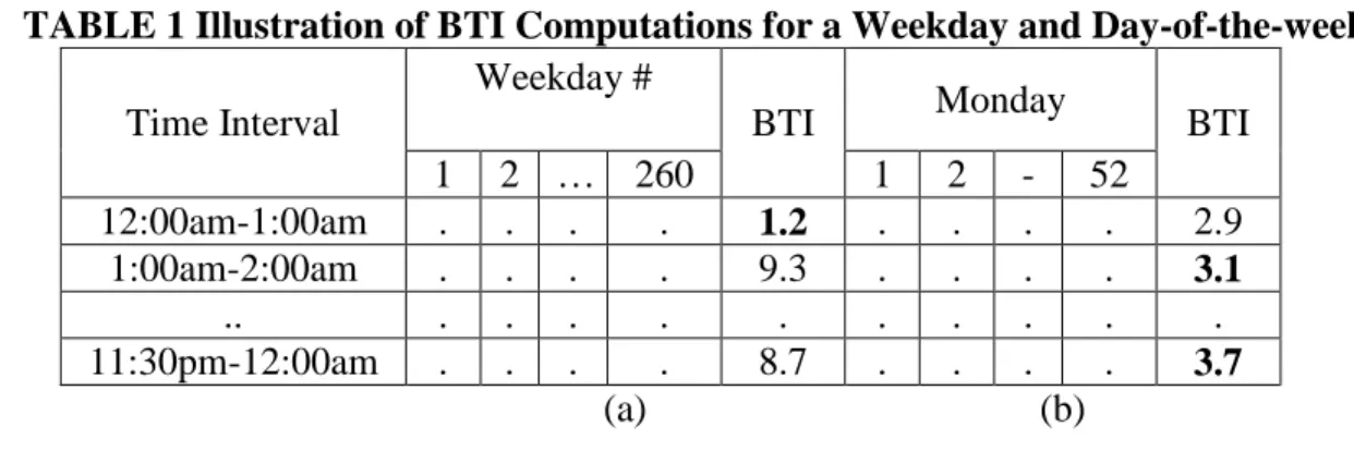
BTIs for two data sets are shown in the Table 1. The part (a) of the Table 1 shows travel 163
times based on the category of a weekday (260 weekdays in year) and part (b) of the Table 1 164
shows for a category day-of-the-week (52 Monday’s in a year) for a given year. From Table 1, 165
one can notice that for each time interval/time-of-the-day (first column) there is an associated 166
BTI (last column). The computed BTI values from the two datasets are used to infer which 167
category is more reliable. BTI for each time interval is compared in the two categories and the 168
category with lower BTI is highlighted, showing it is more reliable for that time interval. But, 169
based on this comparison, it is difficult to judge which category (weekday or Monday) is 170
appropriate or suitable when looking at all the time intervals together (i.e., over a day). This is 171
due to multiple BTI values associated with a link in a category. In other words, it can be said that 172
these indices possess only a one-dimensional ability to measure the reliabilities of links. Also, 173
week-of-the-year was hardly considered in the past studies while addressing reliability. The 174
week-of-the-year, which gives information about the month of the trip, might well influence the 175
travel time (for example, weeks with long weekends). This research introduces and proposes the 176
use of a new performance measures (Cronbach’s α) to evaluate a single index associated for each 177
category (considering week-of-the-year) of travel time data. The proposed performance measure 178
also helps compare which category or group is reliable. 179
180
TABLE 1 Illustration of BTI Computations for a Weekday and Day-of-the-week 181
Time Interval
Weekday #
BTI Monday BTI
1 2 … 260 1 2 - 52 12:00am-1:00am . . . . 1.2 . . . . 2.9 1:00am-2:00am . . . . 9.3 . . . . 3.1 .. . . . 11:30pm-12:00am . . . . 8.7 . . . . 3.7 (a) (b) 182 Data Description 183
The city of Charlotte, in Mecklenburg County, North Carolina is considered as the study area. 184
INRIX travel time data for 296 road links (TMCs) in Charlotte area for the year 2009 was 185
gathered. The data obtained has travel time data aggregated for every one minute interval with 186
other trip characteristics such as date, time, average travel speed, and identified TMC code. The 187
raw data obtained from INRIX was aggregated for every 30 minutes to evaluate travel time 188
reliabilities for the study links for every half-hour intervals (48 intervals) in a day. The associated 189
trip characteristics such as week-of-the-year, day-of-the-week, and weekday/weekend 190
information are also evaluated from the ‘date of trip’ available in INRIX database. 191
192
CRONBACH’S α 193
In statistics, Cronbach’s α is used as a measure of internal consistency or an estimate of 194
reliability of a test. It is a measure of squared correlation between observed scores and true 195
scores (21). In other words, reliability is measured in terms of the ratio of true score variance to 196
observed score variance. The observed score is equal to the true score plus the measurement 197
error. It is assumed that a reliable test should minimize the measurement error so that the error is 198
not highly correlated with the true score. On the other hand, the relationship between true score 199
and observed score should be strong for a test to be a reliable one. The coefficient has been 200
widely used in the fields of psychology, social sciences, and nursing. 201
The following example illustrates the working of Cronbach’s α. Consider a case where 202
one needs to determine the reliability of three questions in measuring an entity, say, analytical 203
ability of five persons with various educational levels. The test is intended to rate the persons 204
based on their ability to analyze a given dataset. Note that the assumption in this case is that the 205
ability depends on one’s education and are testing the reliability of the questions in the test. The 206
results of the test are recorded as shown in Table 2, where scores for questions are recorded as 207
binary variables. 208
209
TABLE 2 Summary of Results from Test Scores 210
Students Questions Total
Q1 Q2 Q3 S.1 0 1 1 2 S.2 0 0 1 1 S.3 0 1 0 1 S.4 0 0 1 1 S.5 1 1 1 3 Item Variances 0.16 (0.19) 0.24 (0.25) 0.16 Variance of Totals 0.64 (0.24) 211 From Table 2, 212
Sum of individual variances (V1) = 0.16 + 0.24 + 0.16 = 0.56 213
Variance of the total scores (V2) = 0.64 214
Number of questions (items; K) = 3 215
216
For the aforementioned problem, Cronbach’s α is computed using the following 217 expression (22). 218
where, K is the number of questions, 219
is the variance of the observed total test scores of a person, and, 220
is the variance of the sums of scores of a question for all the five persons. 221
Based on K and computed V1 and V2 from Table 2, 222
= 0.1875 223
A ‘zero’ value of α indicates that the questions does not measure the same entity, in this 224
case their analytical ability. On the other hand, if α is ‘one’, it indicates that all the questions 225
designed did a perfect job. This happens when the scores of a student remain same for all 226
questions making him score either 3 or 0 in total. The computed Cronbach’s α in the above 227
example is 0.1875, indicating that the questions are very less reliable in measuring the analytical 228
ability of the person. 229
From the above equation, it can be observed that when variance 1 (V1) is greater than (or 230
far less than) variance 2 (V2), a negative value (or value greater than one) for Cronbach’s 231
coefficient is obtained. But, this occurs only when the sample data is incomplete (i.e., when there 232
are missing fields within the data) and V2 is affected. The sample shown in Table 2 demonstrates 233
the occurrence of absurd values in evaluation of Cronbach’s coefficient. When some values in 234
Table 2 are omitted, V1 and V2 are affected (V1 = 0.6; V2 = 0.24) giving a Cronbach’s 235
coefficient of -2.23. In such cases, either the missing cells should be filled with an average value 236
or the sum of the scores (final column in Table 2) should be proportionately increased to 237
accommodate the missing values. The later was applied in the current analysis to counter the 238
incomplete data for the validity of results. However, if the number of missing cells is more, this 239
approach might not fix the issue. 240
In the above example, the persons are the primary source of variance while questions are 241
the secondary source of variance. In our research, time-of-the-day and week-of-the-year are 242
considered as sources of variance, both primary and secondary. Taking one combination at a 243
time i.e., Cronbach’s α is evaluated once with time-of-the-day as primary factor and next with 244
week-of-the-year as primary factor. In general, the primary factor causes the changes in the 245
observations and correlation is evaluated over the secondary factor (test items). 246
In summary, Cronbach’s α measures the correlation between the results coming from 247
various items i.e., the correlation between the columns in the above table or simply, it is the 248
correlation of test with itself. Whereas, gives the index of measurement error (21). 249
250
APPLICATION OF CRONBACH’S α TO ASSESS RELIABILITY 251
Travel time reliability is measured on the basis of various categories of travel times (day-of-the-252
week, weekend/weekday, time-of-the-day, etc.). A sample data of travel times for ‘Monday’ and 253
‘weekday’ category is shown in Table 1 (b). In the table, the ‘week-of-the-year’ corresponds to 254
the secondary factor and the ‘time-of-the-day’ corresponds to the primary factor i.e., the travel 255
time is expected to vary with time-of-the-day and is checked for the consistency (reliability) over 256
the 52 weeks of a given year. A higher value of Cronbach’s α is obtained when the travel times 257
over the day are well correlated between the 52 weeks of the year. The maximum of ‘1’ is 258
obtained when all the 52 weeks have identical travel times for any time interval of the day 259
(maintaining certain variance within the various time intervals of the day). Reliability scores are 260
compared by changing the primary and secondary factors (like transposing rows and columns in 261
Table 1 (b)), and the most reliable groups that give the best expected travel times are identified. 262
263
CASE STUDY 264
A 2-mile section of freeway on I-85 Northbound direction in the city of Charlotte, NC with TMC 265
code ‘125+04629’ is considered as the case study to illustrate the working of the methodology. 266
Travel time data for the year 2009 was considered to evaluate reliability based on two categories 267
- day-of the-week and weekday/weekend. 268
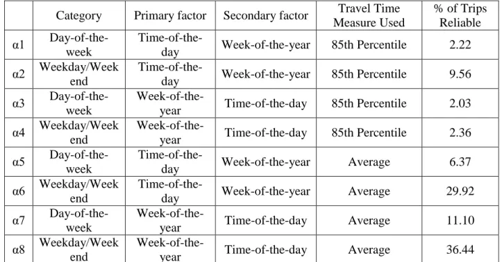
Two different travel time measures, 85th percentile travel times and average travel times, 269
were considered to evaluate reliable trip lengths, hence yielding 8 categories of ‘α’ values as 270
summarized in Table 3. The summary of all the ‘α’ scores computed for the abovementioned 271
TMC code, for each day-of-the-week, are shown in Table 4. 272
273
TABLE 3 Characteristics of Each Category of Cronbach’s ‘α’ 274
Category Primary factor Secondary factor Travel Time Measure Used % of Trips Reliable α1 Day-of-the-week
Time-of-the-day Week-of-the-year 85th Percentile 2.22 α2 Weekday/Week
end
Time-of-the-day Week-of-the-year 85th Percentile 9.56 α3
Day-of-the-week
Week-of-the-year Time-of-the-day 85th Percentile 2.03 α4 Weekday/Week
end
Week-of-the-year Time-of-the-day 85th Percentile 2.36 α5
Day-of-the-week
Time-of-the-day Week-of-the-year Average 6.37
α6 Weekday/Week end
Time-of-the-day Week-of-the-year Average 29.92
α7 Day-of-the-week
Week-of-the-year Time-of-the-day Average 11.10
α8 Weekday/Week end
Week-of-the-year Time-of-the-day Average 36.44
275
TABLE 4 Cronbach’s ‘α’ associated for Varying Categories, 276
Primary and Secondary Factors for a TMC 277
TMC Code DOW WD α1 α2 α3 α4 α5 α6 α7 α8 Max(α) 125+04629 1 0 0.41 0.17 0.53 0.68 0.58 0.18 0.62 0.63 0.68 125+04629 2 1 0.34 0.36 0.12 0.62 0.37 0.38 0.15 0.67 0.67 125+04629 3 1 0.35 0.36 0.52 0.62 0.38 0.38 0.57 0.67 0.67 125+04629 4 1 0.50 0.36 0.75 0.62 0.31 0.38 0.69 0.67 0.75 125+04629 5 1 0.44 0.36 0.60 0.62 0.38 0.38 0.58 0.67 0.67 125+04629 6 1 0.61 0.36 0.49 0.62 0.61 0.38 0.57 0.67 0.67 125+04629 7 0 0.23 0.17 0.67 0.68 0.25 0.18 0.62 0.63 0.68 278
*DOW stands for day-of-the-week with Sunday coded as 1, Monday as 2, and so on 279
*WD represents weekday, coded with 1 for weekday and 0 for weekend 280
281 282 283 284
Cronbach’s α Computed for the ‘Day-of-the-week’ category with ‘Week-of-the-year’ as
285
Primary Factor (α3, α7)
286
‘Week-of-the-year’ is considered as the primary factor and Cronbach’s α is computed for every 287
‘day-of-the-week’ (category). In this case, the assumption is that the primary source of variation 288
in travel times on the link is the ‘week-of–the-year’ associated with the trip. For each day-of-the-289
week, the corresponding values of α (α3 and α7) are reported in the Table 4. 290
It can be observed from Table 4 that Mondays are least reliable with this combination 291
while Wednesdays are the most reliable. Cronbach’s α values lying between [0.9, 1], [0.7, 0.9], 292
[0.5, 0.7], [0.4, 0.5], and [0, 0.4] fall in the categories of A (Excellent), B (Highly Reliable), C 293
(Reliable), D (Poorly Reliable), E (Unreliable) respectively. They are same as those used in other 294
studies related to Cronbach’s α (23, 24). 295
296
Cronbach’s α Computed for the ‘Day-of-the-week’ category with ‘Time-of-the-Day’ as
297
Primary Factor
298
‘Time–of-the-day’ is considered as the primary factor to evaluate the reliability score (α). Hence, 299
the assumption in this case is that the primary variance in the travel times is due to the time-of-300
the-day associated with each trip. One can refer to Table 4 for Cronbach’s α value (α1 and α5) 301
for each week-of-the-day based on varying time-of-the-day. It can be observed from Table 4 that 302
none of the values is greater than 0.7 (on absolute scale) nor comparable to the maximum α value 303
for corresponding days (on relative scale) except for Saturdays where α1 (0.61) and α5 (0.61) are 304
comparable to the maximum α8 (0.67). This indicates that the above combination is not the most 305
reliable for any of the seven days-of-the-week. 306
307
Cronbach’s α Computed for the ‘Weekday/Weekend’ category with Varying Primary Factors
308
The results found after aggregation of data for weekday and weekend are shown as α2, α4, α6, 309
α8 in Table 4. The primary and secondary factors as well as the travel time statistic associated 310
with each ‘α’ are shown in Table 3. 311
The tool and results can be used to predict transportation network condition in the future. 312
As an example, a traveler wants to make a travel plan on 14th of February 2015 between 10:00 313
AM to 10:30 AM on the above mentioned TMC and wants to know his/her travel time. The tool 314
developed from this study uses the following steps to make an expectation. 315
316
1) Identify the day-of-the-week, which is Saturday, a weekend. 317
2) Identify the week-of-the-year, which is 7th week-of-the-year 2015. 318
3) Select the maximum ‘α’ and note the combination associated with the ‘α’. 319
320
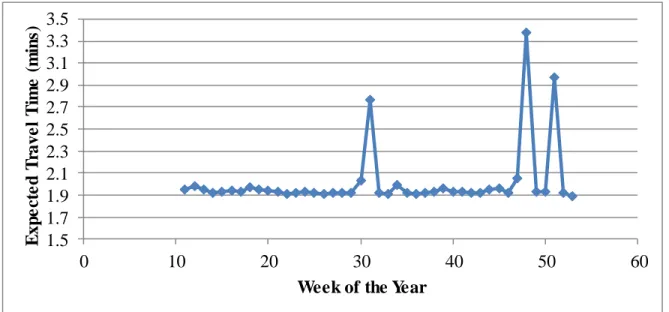
In this case, α4 is the highest. This implies that the category is weekend and the travel 321
time is week-of-the-year dependent (refer Table 3). Hence, one has to take the average of the 85th 322
percentile travel times observed for the weekend category trips for the 7th week-of-the-year. The 323
result gives the expected travel time of the trip. Figure 1 shows the expected travel times (ETT) 324
for weekend category based on the 2009 data with primary factor as ‘week-of-the-year’. One can 325
observe that the ETT depends on the of-the-year with each point representing each week-326
of-the-year in Figure 1 (total 52 points). Since the data is not available for the first 9 weeks of the 327
year, one does not see any points corresponding to them. This shows the limitation of this 328
approach which is further explained in the later sections. However, the basic idea is to compute 329
the Cronbach’s α for all the combinations and take the maximum of these 8 values for any day 330
and then compute the most reliable travel time for any trip. 331 332 1.5 1.7 1.9 2.1 2.3 2.5 2.7 2.9 3.1 3.3 3.5 0 10 20 30 40 50 60 E x p e ct e d T ra v e l T im e ( m in s)
Week of the Year 333
FIGURE 1 Expected travel times for varying week-of-the-year. 334
335
Similarly, analysis to evaluate link-level reliability is applied to all the links considered in 336
the study (296 links). Also, ranking the links with these reliability scores (the maximum of the 8 337
scores is taken for a link) help the traveler choose his/her route from various alternatives. Also, 338
the planning agencies can identify the most unreliable links and make necessary 339
recommendations to improve transportation system performance. The last column of Table 3 340
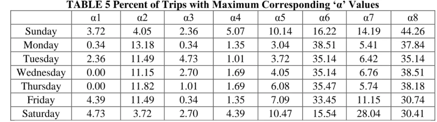
shows the percentage of trips that are reliable for a particular combination associated within α. 341
Table 5 shows the same for each day-of-the-week. It can be observed that a majority of the trips 342
have a higher value of Cronbach’s α when the average travel time values are taken instead of the 343
85th percentile values. Since the data used in the study also involves incidents, the 85th percentile 344
travel time values result in an over-estimation. Additionally, weekday/weekend category 345
grouping ( and ) represent the best expected travel time. This implies that, reliability of a trip 346
depends on whether the trip is on a weekday or weekend rather than a particular day-of-the-347
week. Also, it can be observed that weekday/weekend category grouping with week-of-the-year 348
as primary factor is beneficial for a majority of the weekend trips. This might be because the 349
travel time on a weekend is not much affected by the time-of-the-day as traffic levels are almost 350
equally spread over the day, whereas during weekdays, time-of-the-day is quite defining the 351
travel time. However, the authors do not see a need to generalize here as every link has its own 352
reliable combination to evaluate its reliable travel times. 353
354 355
TABLE 5 Percent of Trips with Maximum Corresponding ‘α’ Values 356 α1 α2 α3 α4 α5 α6 α7 α8 Sunday 3.72 4.05 2.36 5.07 10.14 16.22 14.19 44.26 Monday 0.34 13.18 0.34 1.35 3.04 38.51 5.41 37.84 Tuesday 2.36 11.49 4.73 1.01 3.72 35.14 6.42 35.14 Wednesday 0.00 11.15 2.70 1.69 4.05 35.14 6.76 38.51 Thursday 0.00 11.82 1.01 1.69 6.08 35.47 5.74 38.18 Friday 4.39 11.49 0.34 1.35 7.09 33.45 11.15 30.74 Saturday 4.73 3.72 2.70 4.39 10.47 15.54 28.04 30.41 357
Cronbach’s α Complementing Traditional Reliability Measures
358
With Cronbach’s α measuring the reliability of the link at macro-level and identifying the most 359
reliable base group (category) that closely predicts the travel time, one can use these base groups 360
to compute the traditional reliability measures i.e., BTI and PTI at micro-level. For example, if it 361
is found that weekend travel times are more consistent when the primary factor is the week-of-362
the-year, then BTIs can be evaluated for each week-of-the-year. It can be observed that these 363
BTIs will be much lower than the BTIs that are computed with time-of-the-day as the base group 364
(category). Lower BTIs imply that those set of travel time values are more consistent within 365
themselves. This way Cronbach’s α can be used to compute lower BTIs by changing their base 366
groups or combinations. This also serves as the justification of this study. 367
Figure 2 shows the comparison of the BTIs evaluated for different values of ‘α’ for the same 368
example discussed earlier. While calculating BTI, only 4 cases arise instead of 8 (since BTI 369
needs only these categories). Figure 2(a) and Figure 2(c) represent the BTIs for the trips for 370
every half-hour interval of the day (time-of-the-day category). While Figure 2(a) represents 371
Saturday, Figure 2(c) represents weekend. Similarly, Figure 2 (b) and Figure 2(d) are for week-372
of-the-year category. Figure 2 (b) represents Saturday and Figure 2 (d) represents weekend. 373
From Table 2, since α4 and α8 values are 0.68 and 0.63, respectively which are with the 374
combination of ‘weekend’ category and ‘week-of-the-year’ as primary factor, the associated 375
BTIs are seen close to zero in Figure 2(d) than the others. One can compare these with the BTIs 376
associated with minimum ‘α’ values (α2 and α4) i.e., Figure 2(b). The number of BTIs greater 377
than 10 is more in this case than the other three cases. This reinforces the concept of Cronbach’s 378
α complementing the traditional measures. It is to be noted that the negative values of BTI in 379
Figure 2 indicates the samples with average travel time greater than 95th percentile due to their 380
small size and presence of outliers. 381
382
FIGURE 2 Comparison of BTIs evaluated by Category of Trips. 383
384
Level of Reliability Based on Value of Cronbach’s α
385
Cronbach’s α was used as a performance measure to classify the links/corridors into various LOS 386
categories. Since it is a correlation coefficient, the same threshold values that are used to 387
determine the level of dependence (linear) for various classifications were used. If any of the ‘α’ 388
is greater than 0.9, the link is said to be very highly reliable for the associated combination and 389
one can expect the value to be at least greater than 0.7 to comment on its reliability. From the 390
complete analysis performed in this study, covering 296 links in the city of Charlotte for the year 391
2009 consisting around 2,072 different types of trips based on day-of-the-week (296*7 = 2,072), 392
it is observed that 49.13% of TMCs fall in LOS A category, 37.4% in LOS B category, 12.26% 393
in LOS C category, 0.92% in LOS D Category, and 0.29% in LOS E category. 394
395
Missing Data and Possible Inaccuracies 396
Data availability is one of the major requirements for accurate estimates of reliability scores. The 397
formula used to evaluate Cronbach’s α uses variance 1 (V1) which is the sum of item variances 398
and variance 2 (V2) which is the variance of total scores. The lower the ratio of V1 to V2, the 399
higher is Cronbach’s α. It is to be noted that lower value of V1 should automatically reflect 400
lower value of V2 because when individual values are closer to each other, the sums of those 401
scores should also be closer unless and until some values are missing. In case of missing fields, 402
an over-estimation or under-estimation of Cronbach’s α values is observed. If the variance 2 403
(V2) can be adjusted when missed data is observed, the results can be more credible. Hence, sum 404
of the item scores is proportionately increased to accommodate for all the missing data and to 405
ensure that V2 is a valid representation of the sample. However, the authors understand that this 406
may not depict the true sample but shall improve the validity of the results. The proposed method 407 -30 -20 -10 0 10 20 0 10 20 30 40 50 60 B u ff er T im e In d ex
Nth Half an Hour Interval of the Day (a) α = 0.23 BTI 0 50 100 150 200 250 300 0 10 20 30 40 50 60 B u ff er T im e In d ex
Week of the Year (b) α = 0.17 BTI -15 -10 -5 0 5 10 0 10 20 30 40 50 60 B u ff er T im e In d ex
Nth Half an Hour Interval of the Day (c) α = 0.67 BTI -20 -15 -10 -5 0 5 10 0 10 20 30 40 50 60 B u ff er T im e In d ex
Week of the Year (d)
α = 0.68
has fixed the issue to a large extent though there might be little over-estimation or under-408
estimation in case of missing fields. 409
410
CONCLUSIONS 411
Reliability of a link is crucial to both the users and practitioners of transportation systems. A new 412
reliability measure, Cronbach’s α, is proposed to assess reliability of links in the transportation 413
network. This performance measure acts as a macro-level measure of reliability that evaluates 414
the level of consistency of travel times. The proposed reliability measure was found to be a better 415
estimator of expected travel times as compared to the traditional travel time performance 416
measures such as BTI and PTI, which are often evaluated for a fixed criteria (time-of-the-day). 417
This is because the proposed macroscopic measure evaluated reliability not only for a time-of-418
the-day over the year but also for a week-of-the-year over the time-of-the-day and using both 419
85th percentile travel times as well as average travel times from the historical data. The 420
reliabilities are evaluated at link-level which also helps identify the most unreliable links in the 421
network. 422
Overall, results indicate that the average travel times of the trips aggregated for any time 423
interval from the data yields in more reliable estimates than compared to 85th percentile travel 424
times. Also, weekend trips are not time dependent but are week-of-the-year dependent whereas 425
weekday trips are time dependent in most of the cases. Results also indicate that missing field in 426
the data might result in over- or under-estimation of results. 427
Along with identifying the reliable travel times and reporting absolute reliable scores of 428
the links, a new reliability criteria based on Cronbach scores is proposed. However, a link with 429
LOS ‘A’ from this study does not mean a perfect case, as the travel times associated might still 430
be very high just that they are reliable and recurring. 431
432
ACKNOWLEDGEMENTS 433
This paper is prepared based on information collected for a research project funded by 434
the United States Department of Transportation - Office of the Assistant Secretary for Research 435
and Technology (USDOT/OST-R) under Cooperative Agreement Number RITARS-12-H-436
UNCC. The support and assistance by the project program manager and the members of 437
Technical Advisory Committee in providing comments on the methodology are greatly 438
appreciated. The contributions from other team members at the University of the North 439
Carolina at Charlotte are also gratefully acknowledged. Special thanks are extended to Ms. 440
Kelly Wells of North Carolina Department of Transportation (NCDOT) and Mr. Michael 441
VanDaniker of the University of Maryland (UMD) for providing access and help with INRIX 442 data. 443 444 DISCLAIMER 445
The views, opinions, findings, and conclusions reflected in this paper are the responsibility of the 446
authors only and do not represent the official policy or position of the USDOT/OST-R, NCDOT, 447
UMD, INRIX, or any other State, or the University of North Carolina at Charlotte or other entity. 448
The authors are responsible for the facts and the accuracy of the data presented herein. This 449
paper does not constitute a standard, specification, or regulation. 450
451 452 453
REFERENCES 454
1. Hartgen, D. T., and R. K. Karanam. More to Do: Performance of State Highway Systems
455
1984-2004. 15th Annual Report, Reason Foundation, Los Angeles CA, October 4, 2006. 456
2. Hartgen, D. T. Traffic Congestion in North Carolina: Status, Prospects and Solutions. John 457
Locke Foundation, 2007. 458
3. Federal Highway Administration. Travel Time Reliability: Making It There On Time, All the
459
Time. www.ops.fhwa.dot.gov/publications/tt_reliability/TTR_Report.htm. Accessed July 14, 460
2007. 461
4. Iida, Y., and H. Wakabayashi. An Approximation Method of Terminal Reliability of Road 462
Network using Partial Minimal Path and Cut Sets. Transport Policy, Management & 463
Technology towards 2001: Selected Proceedings of the Fifth World Conference on Transport 464
Research, Vol. 4, 1989. 465
5. Recker, W., Y. Chung, J. Park, L. Wang, A. Chen, Z. Ji, H. Liu, M. Horrocks, and J. S. Oh. 466
Considering Risk-taking Behavior in Travel Time Reliability. California PATH Research 467
Report, UCB–ITS–PRR–2005-3, U. S. Department of Transportation, 2005. 468
6. Asakura, Y., and M. Kashiwadani. Road Network Reliability Caused by Daily Fluctuation of 469
Traffic Flow. PTRC Summer Annual Meeting, University of Sussex, United Kingdom, 1991. 470
7. Nicholson, A., and Z. P. Du. Degradable Transportation Systems: An Integrated Equilibrium 471
Model. Transportation Research Part B: Methodological, Vol. 31(3), 1997, pp. 209-223. 472
8. Chen, A., H. Yang, H. K. Lo, and W. H. Tang. Capacity Reliability of a Road Network: An 473
Assessment Methodology and Numerical Results. Transportation Research Part B:
474
Methodological, Vol. 36(3), 2002, pp. 225-252. 475
9. Heydecker, B. G., W. H. K. Lam, and N. Zhang. A New Concept of Travel Demand 476
Satisfaction Reliability for Assessing Road Network Performance. Matsuyama Workshop on 477
Transport Network Analysis, Matsuyama, Japan, 2000. 478
10.Small, K. A. The Scheduling of Consumer Activities: Work Trips. American Economic 479
Review, Vol. 72(3), 1982, pp. 467-479. 480
11.Chen, A., Z. Ji, and W. Recker. Effect of Route Choice Models on Estimation of Travel Time 481
Reliability under Demand and Supply Variations. Network Reliability of Transport. 482
Proceedings of the 1st International Symposium on Transportation Network Reliability 483
(INSTR), 2003. 484
12.Abdel-Aty, M., A., R. Kitamura, and P. P. Jovanis. Investigating Effect of Travel Time 485
Variability on Route Choice using Repeated-Measurement Stated Preference Data. 486
Transportation Research Record, No. 1493, 1999, pp. 39-45. 487
13.Haitham M., A. D. and B. Emam. New Methodology for Estimating Reliability in 488
Transportation Networks with Degraded Link Capacities. Journal of Intelligent
489
Transportation Systems, Vol. 10(3), 2006, pp. 117-129. 490
14.Heydecker, B. G., W. H. K. Lam, and N. Zhang. Use of Travel Demand Satisfaction to 491
Assess Road Network Reliability. Transportmetrica, Vol. 3(2), 2007, pp. 139-171. 492
15.Chen, A., J. Kim, S. Lee, and Y. Kim. Stochastic Multi-objective Models for Network 493
Design Problem. Expert Systems with Applications, Vol. 37(2), 2010, pp. 1608-1619. 494
16.Douglas S. M., and G. Morgan. The Florida Reliability Method in Florida’s Mobility 495
Performance Measures Program. Florida Department of Transportation, 2000. 496
17.Federal Highway Administration (FHWA). Travel Time Reliability: Making it There on
497
Time, all the Time. Federal Highway Administration, United States Department of 498
Transportation, 2006. http://www.ops.fhwa.dot.gov/publications/tt_reliability/index.htm 499
FHWA Report. Accessed July 31, 2014. 500
18.Clark, S., and D. Watling. Modelling Network Travel Time Reliability under Stochastic 501
Demand. Transportation Research Part B: Methodological, Vol. 39(2), 2005, pp. 119-140. 502
19.Higatani, A., T. Kitazawa, J. Tanabe, Y. Suga, R. Sekhar, and Y. Asakura. Empirical 503
Analysis of Travel Time Reliability Measures in Hanshin Expressway Network. Journal of
504
Intelligent Transportation Systems, Vol. 13(1), 2009, pp. 28-38. 505
20.Bates, J., J. Polak, P. Jones, and A. Cook. The Valuation of Reliability for Personal Travel. 506
Transportation Research Part E: Logistics and Transportation Review, Vol. 37(2), 2001, pp. 507
191-229. 508
21.Yu, C. H. An Introduction to Computing and Interpreting Cronbach Coefficient Alpha in 509
SAS. Proceedings of 26th SAS User Group International Conference, 2001. 510
22.Cronbach, L. J., Coefficient Alpha and the Internal Structure of Tests. Psychometrika, Vol. 511
16, 1951, pp. 297–333. 512
23.George, D., and P. Mallery. SPSS for Windows Step by Step: A Simple Guide and Reference 513
11.0 update, 4th ed., 2003, Boston: Allyn and Bacon. 514
24.Kline, P. The Handbook of Psychological Testing, 2nd ed., page 13, 2000, London: 515
Routledge. 516