A Parallel Formulation of the Spatial Auto-Regression Model for Mining Large Geo-Spatial Datasets Abstract: Keywords: 1 Introduction.

A Parallel Formulation of the Spatial Auto-Regression Model for Mining

Large Geo-Spatial Datasets

Baris M. Kazar

, Shashi Shekhar

, David J. Lilja*, Daniel Boley

The spatial auto-regression model (SAM) is a popular spatial data mining technique which has been used in many applications with geo-spatial datasets. However, serial procedures for estimating SAM parameters are computationally expensive due to the need to compute all the eigenvalues of a very large matrix. We propose a parallel formulation of the SAM parameter estimation procedure in this paper using data parallelism and hybrid programming technique. Experimental results on an IBM Regatta show that the proposed parallel formulation achieves a speedup of up to 7 on 8 processors. We are developing algebraic cost models to analyze the experimental results to further improve the speedups. Keywords: Spatial regression, Spatial Auto-correlation, Parallel Formulation, Spatial Data Mining 1 Introduction.

Explosive growth in the size of spatial databases has highlighted the need for spatial data mining techniques to mine the interesting but implicit spatial patterns within these large databases. Extracting useful and interesting patterns from massive geo-spatial datasets is important for many application domains such as regional economics, ecology and environmental management, public safety, transportation, public health, business, and travel and tourism [2,13,14].

Many classical data mining algorithms such as linear regression assume that the learning samples are

independently and identically distributed (IID). This

assumption is violated in the case of spatial data due to

spatial auto-correlation [14] and classical linear

regression yields a weak model with not only low prediction accuracy [13] but also residual error exhibiting spatial dependence.

† _{This work was partially supported by the Army High}

Performance Computing Research Center (AHPCRC) under the auspices of the Department of the Army, Army Research Laboratory (ARL) under contract number DAAD19-01-2-0014. This work received additional support from the University of Minnesota Digital Technology Center and the Minnesota Supercomputing Institute.

‡

Electrical and Computer Engineering Department, University of Minnesota, Twin-Cities MN 55455, Email:[email protected] §

Computer Science and Engineering Department, University of Minnesota, Twin-Cities MN 55455, Email: [email protected] * Electrical and Computer Engineering Department, University of Minnesota, Twin-Cities MN 55455, Email: [email protected] ¶

Computer Science and Engineering Department, University of Minnesota, Twin-Cities MN 55455, Email: [email protected]

The spatial auto-regression model (SAM) [5,14] is a generalization of the linear regression model to account for spatial auto-correlation. It has been successfully used to analyze spatial datasets in regional economics, ecology [2,13], etc. The model yields better classification and prediction accuracy [2,13] for many spatial datasets exhibiting strong spatial auto-correlation.

However, it is computationally expensive to estimate the parameters of SAM. For example, it can take an hour of computation for a spatial dataset with 10000 observation points on an IBM Regatta 32- processor node composed of 1.3GHz pSeries 690 Power4 architecture processors sharing 47.5 GB main memory. This has limited the use of SAM to small problems, despite its promise to improve classification and prediction accuracy for larger spatial datasets. Parallel processing is a promising approach to speedup the sequential solution procedure for SAM and this paper focuses on this approach.

The only related work [9] implemented the SAM solution for one-dimensional geo-spaces and used CMSSL [4], a parallel linear algebra library written in CM-Fortran (CMF) for the CM-5 supercomputers of Thinking Machines Corporation, neither of which is available for use anymore. That approach was not useful for spatial datasets embedded in spaces of two or more dimensions. Thus, it is not included in comparative evaluation in this paper.

We propose a parallel formulation for a general exact estimation procedure [6] for SAM parameters that can be used for spatial datasets embedded in multi-dimensional space. We use a public domain parallel numerical analysis library to implement the steps of the serial solution on an SMP architecture machine, i.e., a single node of an IBM Regatta. To tune the performance, we modify the source code of the library to change parameters such as scheduling and data-partitioning.

We evaluate the proposed parallel formulation on an IBM Regatta. Results of experiments show that the proposed parallel formulation achieves a speedup of up to 7 on 8 processors within a single node of the IBM Regatta. We compare different load-balancing tech-niques supported by OpenMP [1] for improving the speedup of the proposed parallel formulation of SAM. Affinity scheduling, which is both a static and dynamic (i.e., quasi-dynamic) load-balancing technique, performs best on average. We also evaluate the impact of other OpenMP parameters, i.e. chunk size defined as the number of iterations per scheduling step.

We plan to expand the experimental studies to include a larger number of processors via hybrid parallel

programming, and other parameters such as degree of auto-correlation. To further improve speedup we also plan to develop algebraic cost models to characterize the scalability and identify the performance bottlenecks.

Eventually, we want to develop parallel formulations for approximate solution procedures for SAM that exploit sparse matrix techniques [8].

Scope: This paper covers parallel formulation for a

dense and exact solution to SAM. The parallel SAM

solution is portable and can run on today’s distributed shared-memory architecture supercomputers such as IBM Regatta, SGI Origin, SGI Altix, and Cray X1. We do not address non-parallel approaches, e.g., sparse matrix techniques and approximation techniques, to speedup the sequential solutions to SAM.

The remainder of the paper is organized as follows: Section 2 presents the problem statement and explains the serial exact algorithm for the SAM solution. Section 3 discusses our parallel formulation. Experimental results are presented in Section 4. Finally, Section 5 summarizes and concludes the paper with a discussion of future work.

2 Problem Statement and Serial Exact SAM Solution.

We first present the problem statement and then discuss the serial exact SAM solution based on the maximum-likelihood (ML) theory [6].

The problem studied in this paper is defined as follows: Given the serial solution procedure described in the Serial Dense Matrix Approach [9], we need to find a parallel formulation for multi-dimensional geo-spaces to reduce the response time. The constraints are as follows: the spatial auto-regression parameter,ρ, varies in the range [0,1); the error is normally distributed, i.e. εεεε

∼N(0,σ2_{I) IID; the input spatial dataset is composed of}

normally distributed random numbers with unit standard deviation and zero mean; the parallel platform is composed of an IBM Regatta, OpenMP and MPI; and the size of the neighborhood matrix W is n. The

objective is to implement parallel and portable software

whose scalability is evaluated analytically and experimentally.

A spatial auto-correlation termρWy is added to the linear regression model in order to model the strength of the spatial dependencies among the elements of the dependent variable, y. The resulting equation – which accounts for the spatial relationships – is shown in equation 2.1 and is called the spatial auto-regression

model (SAM) [5].

(2.1) ε

xβ

Wy

y=ρ + +

where ρis the spatial auto-regression (auto-correlation) parameter, y is an n-by-1 vector of observations on the

dependent variable, x is an n-by-k matrix of observations on the explanatory variable, W is the n-by-n neighborhood matrix that accounts for the spatial relationships (dependencies) among the spatial data, βis a k-by-1 vector of regression coefficients, ε is an n-by-1

vector of unobservable error.

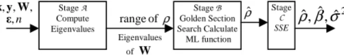
Figure 1. System diagram of the serial exact algorithm for the SAM

solution composed of three stages, Stage A, B, and C. Stage A is further

composed of three sub-stages (pre-processing, Householder transformation and QL transformation) which are not shown.

Figure 1 highlights the stages of the serial exact algorithm for the SAM solution. It is based on maximum-likelihood (ML) theory, which requires computing the logarithm of the determinant of the large

)

(I−ρ W matrix. The derivation of the ML theory will not

be shown here due to limited space. However, the first term of the end-result of the derivation of the logarithm of the likelihood function i.e. equation 2.2 clearly shows why we need to compute the (natural) logarithm of the determinant of a large matrix. In equation 2.2 the n-by-n identity matrix is denoted by “I”, the transpose operator is denoted by “T”, “ln” denotes the logarithm operator and _σ2 _{is the common variance of the error.}

(2.2) L = − −n −n −SSE 2 ) ln( 2 ) 2 ln( ln ) ln( 2 σ π ρW I

{

}

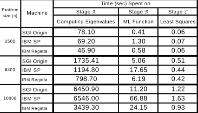
Therefore, Figure 1 can be viewed as an implementation of the ML theory. This section describes each stage. Stage A is composed of three sub-stages: pre-processing, Householder transformation [11], and QL transformation [3]. The pre-processing sub-stage not only forms the row-standardized neighborhood matrix W, but also converts it to its symmetric eigenvalue-equivalent matrixW~ . The Householder transformation and QL transformation sub-stages are used to find all of the eigenvalues of the neighborhood matrix. The Householder transformation sub-stage takes W~ as input and forms the tri-diagonal matrix whose eigenvalues are computed by the QL transformation sub-stage. Computing all of the eigenvalues of the neighborhood matrix takes approximately 99% of the total serial response time as shown in Table 1.

Stage B uses the eigenvalues of the neighborhood matrix to calculate the determinant of (I−ρ W) at each step of the non-linear one-dimensional parameter optimization using the golden section search [3]. The value of the

Stage B Golden Section Search Calculate ML function Stage A Compute Eigenvalues Stage C SSE n , , , ,yε W x Eigenvalues of W ρˆ _ˆ2 , ˆ , ˆ β σ ρ ρ of range

logarithm of the likelihood function (equation 2.2) needs to be computed at each iteration step of the non-linear optimization because the auto-regression parameter is updated at each step. There are two ways to compute the value of the logarithm of the likelihood function: 1) compute the eigenvalues of the large dense matrix W

once; 2) compute the determinant of the large dense matrix (I−ρ W) at each step of the non-linear

optimization. Due to space limitations, it is enough to note that the former option takes less execution time for large problem sizes, i.e., for large number of observation points. Equation 2.3 expresses the relationship between the eigenvalues of the W matrix and the logarithm of the determinant of the (I−ρ W) matrix. The optimization is O(n) complexity. (2.3) ∑ = − = −     →  ∏ = − = − n i i ρλ ρ n i i ρλ ρ 1 ) ln(1 | | ln 1 ) (1 | | logarithm the taking W I W I

Finally, stage C computes the sum of the squared error, i.e., the SSE term, which is O(n2) complex. Table 1 shows our measurements of the serial response times of the stages of the exact SAM solution based on ML theory. Each response time given in this study is the average of five runs. We note that stage A takes a large fraction of the total time.

Table 1. Measured serial response times of stages of the exact

SAM solution. Problem size denotes the number of observation points

Stage A Stage B Stage C Com puting Eigenvalues ML Function Least Squares SGI Origin 78.10 0.41 0.06 IBM SP 69.20 1.30 0.07 IBM Regatta 46.90 0.58 0.06 SGI Origin 1735.41 5.06 0.51 IBM SP 1194.80 17.65 0.44 IBM Regatta 798.70 6.19 0.42 SGI Origin 6450.90 11.20 1.22 IBM SP 6546.00 66.88 1.63 IBM Regatta 3439.30 24.15 0.93

Tim e (sec) Spent on

2500

6400

10000 Problem

size (n) Machine

3 Our Parallel Formulation.

The parallel SAM solution implemented here uses a data-parallelism approach such that each processor works on different data with the same instructions. Data parallelism is chosen since it provides finer granularity for parallelism than functional parallelism.

3.1 Stage AAAA: Computing Eigenvalues. Stage A can be parallelized using parallel eigenvalue solvers [7,10,12]. If the source code of the parallel eigenvalue solver is available, the code may be modified in order to tune the performance by changing the parameters such as scheduling technique and chunk size.

We use a public domain parallel eigenvalue solver from the Scalapack Library [12]. This library is available on MPI-based communication paradigm. Thus, we use a hybrid programming technique to exploit this library within OpenMP, a shared memory programming model which is preferred within each node of the IBM Regatta. In future work, we will use OpenMP within nodes and MPI across nodes of the IBM Regatta. We modified the source code of the parallel eigensolver within Scalapack to allow evaluation of different design decisions including the choice of scheduling techniques and chunk sizes. OpenMP provides a rich set of choices for scheduling techniques i.e., static, dynamic, guided, and affinity scheduling techniques.

Another important design decision relates to the partitioning of data items. We instructed OpenMP to partition the neighborhood matrix across processors. 3.2 Stage BBBB: Fitting for the Autoregression Parameter. The golden section search algorithm itself is left un-parallelized since it is very fast in serial format and the response time may increase due to the communication overhead. The serial golden section search stage has linear complexity. However, the golden section search needs to compute the logarithm of the maximum-likelihood function, all of whose constant (spatial statistics) terms are computed in parallel.

spatial auto-regression model, is calculated in parallel. The formula for βˆ _{is derived from ML theory. The}

estimate of the common variance of the error term _σˆ2_is

also computed in parallel to compare with the actual value. The complexity is reduced to O(n2/p) from O(n2) due to the parallelization of this stage.

4 Experimental Design.

Our experimental design answers four important questions by using synthetic data-sets:

1.Which load-balancing method provides best speedup? 2.How does problem size i.e., the number of observation

points (n) affect speedup?

3.How does chunk size i.e., the number of iterations per scheduling step (B) affect speedup?

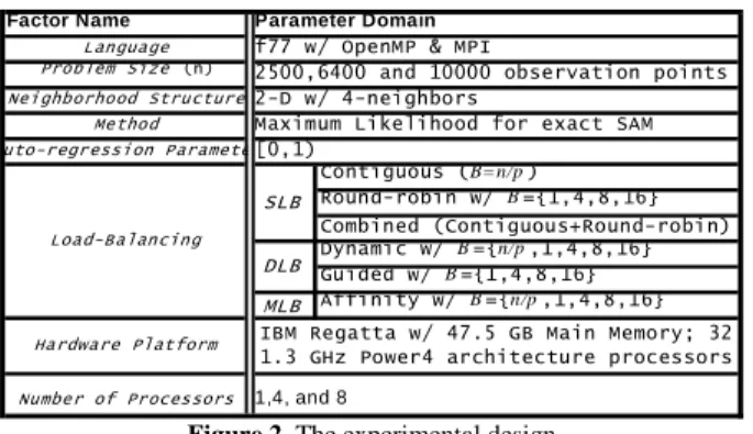
4.How does number of processors (p) affect speedup? Figure 2 summarizes the factors and their parameter domains. The most important factors are load-balancing technique, problem size, chunk-size and number of processors. These factors determine the performance of the parallel formulation. We used 4 neighbors in the neighborhood structure, but 8 and more neighbors could also be used. The load-balancing techniques of OpenMP can be grouped in four major classes:

1. Static Load-Balancing (SLB)

• Contiguous Scheduling: Since B is not specified, the iterations of a loop are divided into chunks of n/p iterations each. We refer to this scheduling as static

B=n/p.

• Round-robin Scheduling: The iterations are

distributed in chunks of size B in a cyclic fashion. This scheduling is referred to as static B={1,4,8,16}. 2. Dynamic Load-Balancing (DLB)

• Dynamic Scheduling: If B is specified, the iterations of a loop are divided into chunks containing B iterations each. If B is not specified, then the chunks consist of n/p iterations. The processors are assigned these chunks on a "first-come, first-do" basis. Chunks of the remaining work are assigned to available processors.

• Guided Scheduling: If B is specified, then the iterations of a loop are divided into progressively smaller chunks until a minimum chunk size of B is reached. The default value for B is 1. The first chunk contains n/p iterations. Subsequent chunks consist of

number of remaining iterations divided by p

iterations. Available processors are assigned chunks on a "first-come, first-do" basis.

3. Quasi-Dynamic Load-Balancing composed of both static and dynamic components (QDLB).

• Affinity Scheduling: The iterations of a loop are initially divided into p chunks, containing n/p iterations. If B has been specified, then each processor is initially assigned to a chunk, and is then further subdivided into chunks containing B iterations. If B has not been specified, then the chunks consist of half of the number of iterations

remaining iterations. When a thread becomes free, it takes the next chunk from its initially assigned partition. If there are no more chunks in that partition, then the thread takes the next available chunk from a partition initially assigned to another thread.

4. Mixed Load-Balancing:

• Mixed1 and Mixed2 Schedulings: Composed of both static and round-robin scheduling

The first response variable is speedup and is defined as the ratio of the serial execution time to the parallel execution time. The second response variable, parallel

efficiency, is a metric that is defined as the best speedup number obtained on 8 processors divided by 8. The standard deviation of five runs reported in our experiments for problem size 10000 is 16% of the average run-time (i.e. 561 seconds). It is 9.5% (i.e. 76 seconds) of the average run-time for problem size 6400 and 10.6% of the average run-time (i.e.5.2 seconds) for problem size 2500. Factor Name Language Problem Size (n) Neighborhood Structure Method Auto-regression Parameter Contiguous (B=n/p) Round-robin w/ B={1,4,8,16} Combined (Contiguous+Round-robin) Dynamic w/ B={n/p,1,4,8,16} Guided w/ B={1,4,8,16} MLB Affinity w/ B={n/p,1,4,8,16} Number of Processors

Maximum Likelihood for exact SAM [0,1)

SLB DLB

Parameter Domain f77 w/ OpenMP & MPI

2500,6400 and 10000 observation points 2-D w/ 4-neighbors

IBM Regatta w/ 47.5 GB Main Memory; 32 1.3 GHz Power4 architecture processors Hardware Platform

1,4, and 8

Load-Balancing

Figure 2. The experimental design

4.1 Which load-balancing method provides the best speedup? Experimental Setup: The response variables are speedup and parallel efficiency. Even though the neighborhood structure used is the 4-nearest neighbors for multi-dimensional geo-spaces, our method can solve for any type of neighborhood matrix depending on different structures.

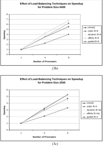
Trends: Figure 3 summarizes the average speedup results for different load-balancing techniques. For each problem size, affinity scheduling appears to be the best. For example, in Figure 3(a) affinity scheduling with chunk-size 1 provides best speedup. In Figure 3(b) for problem size 6400, affinity scheduling with chunk-size 8 provides best speedup. Affinity scheduling with chunk-size n/p provides best speedup in Figure 3(c) for problem size 2500. The main reason is that affinity scheduling does scheduling both at compile time and run-time, allowing it to adapt quickly to the dynamism in the program without much overhead. Results show that the parallel efficiency increases as the problem size increases. The best parallel efficiency obtained for problem size 10000 is 93.13%, while for problem size 6400, it is 83.45%; and for problem size 2500 it is 66.26%. This is due to the fact that as the problem size increases, the ratio of parallel time spent in the code to the serial time spent also increases.

Effect of Load-Balancing Techniques on Speedup for Problem Size 10000

0 1 2 3 4 5 6 7 8 1 4 8 Number of Processors S p e e d u p mixed1 Static B=8 Dynamic B=8 Affinity B=1 Guided B=16 (3a)

Effect of Load-Balancing Techniques on Speedup for Problem Size 6400

0 1 2 3 4 5 6 7 8 1 4 8 Number of Processors S p e e d u p mixed1 static B=8 dynamic B=8 affinity B=8 guided B=8 (3b)

Effect of Load-Balancing Techniques on Speedup for Problem Size 2500

0 1 2 3 4 5 6 1 4 8 Number of Processors S p e e d u p mixed1 static B=4 dynamic B=16 affinity B=n/p gudied B=4 (3c)

Figure 3. The best speedup results from each class of load-balancing techniques (i.e. mixed1, mixed2, static w/o B, with B={1,4,8,16}; dynamic with B={n/p,1,4, 8,16}; affinity w/o B, with B={1,4,8,16}; guided w/o B or with B=n/p, and B={4,8,16) for problem sizes (n) a) 10000, b) 6400 and c)2500 on 1,4 and 8 processors. Mixed1 scheduling uses static with B=4 (round-robin w/ B=4) for non-uniform workload and static w/o B (contiguous) for uniform workload. Mixed2 scheduling uses static with B=16 (round-robin w/ B=16) for non-uniform workload and static w/o B (contiguous) for non-uniform workload.

4.2 How does problem size impact speedup?

Experimental Setup: The number of processors is fixed at 8 processors. The best and worst load-balancing techniques, namely affinity scheduling and guided scheduling, are presented as two extremes. Speedup is the response variable. The chunk-sizes and problem sizes are varied. Recall that chunk size is the number of iterations per scheduling step and problem size is the number of observation points.

Trends: The two extremes for the load-balancing techniques are shown in Figure 4. In the case of affinity scheduling the speedup increases linearly with problem size. In the case of guided scheduling, even though the increase in speedup is not linear as the problem size increases, there is still some speedup. An interesting trend for affinity scheduling with chunk size 1 is it starts as the worst scheduling but then moves ahead of every other scheduling when the problem size is 10000 observation points. Since we ran out of memory for

problem sizes greater than 10000 due to the quadratic growth in W matrix, we were unable to observe whether this trend is maintained for larger problem sizes.

4.3 How does chunk-size affect speedup?

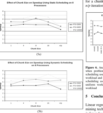
Experimental Setup: The response variable is the speedup. The number of processors is fixed at 8 processors. The problem sizes and the chunk sizes are varied. We want to compare two load-balancing techniques, static scheduling and dynamic scheduling. Static scheduling is arranged only at compile time, while dynamic scheduling is arranged only at run-time.

Trends: Figure 5 presents the comparison. As can be seen, there is a value of chunk size between 1 and

n/p that results in the highest speedup for each load-balancing scheme. The dynamic scheduling reaches the maximum speedup when chunk size is 16, while static scheduling reaches the maximum speedup at chunk size 8. This is due to the fact that dynamic scheduling needs more work per processor in order to beat the scheduling overhead. There is a critical value of the chunk size for which the speedup reaches the maximum. This value is higher for dynamic scheduling to compensate for the scheduling overhead. The workload is more evenly distributed across processors at the critical chunk size value.

Impact of P roblem Siz e on Speedup U sing Affinity S cheduling on 8 P rocessors 0 1 2 3 4 5 6 7 8 2500 6400 10000 P roble m S ize S p e e d u p affinity B =n/p affinity B =1 affinity B =4 affinity B =8 afiinity B =16 (4a)

Impact of Problem Size on Speedup Using Guided Scheduling on 8 Processors 0 1 2 3 4 5 6 2500 6400 10000 Problem Size S p e e d u p Guided B=1 Guided B=4 Guided B=8 Guided B=16 (4b)

Figure 4. Impact of problem size on speedup using a) affinity and b) guided scheduling on 8 processors.

Effect of Chunk Size on Speedup Using Static Scheduling on 8 Processors 0 1 2 3 4 5 6 7 8 1 4 8 16 n/p Chunk Size S p e e d u p PS=2500 PS=6400 PS=10000 (5a)

E ffect of C hun k S iz e on S p eedup U sin g D ynam ic S chedu ling on 8 P roce ssors 0 1 2 3 4 5 6 7 8 1 4 8 16 n/p Chunk S iz e S p e e d u p P S = 2500 P S = 6400 P S = 10000 (5b)

Figure 5. Effect of chunk size on speedup using a) static and b) dynamic schedulings on 8 processors.

4.4 How does number of processors affect speedup?

Experimental Setup: The chunk size is kept constant at 8 and 16. Speedup is the response variable. The number of processors is varied i.e. {4, 8}. The problem size is fixed at 10000 observation points. Due to the limited budget of computational time available on IBM Regatta, we did not explore other values for the number of processors.

Trends: As Figure 6 shows, the speedup increases as the number of processors goes from 4 to 8. The average speedup across all scheduling techniques is 3.43 for the 4-processor case and 5.91 for the 8-processor case. Affinity scheduling shows the best speedup, on average 7 times on 8 processors. Therefore, the speedup increases as the number of processors increases. Guided scheduling results in the worst speedup because the first processor is always assigned a chunk of size n/p. The rest of the processors always have less work to do even though the rest of the work can be distributed evenly. The same scenario applies to static scheduling with chunk size n/p. Dynamic scheduling tends to result in better speedup as the chunk size increases. However, it also suffers from the same problem of guided and static scheduling techniques when the chunk size is n/p. Therefore, we expect dynamic scheduling will have its best speedup

for a chunk size which is somewhere between 16 and

n/p iterations.

Effect of Number of Processors on Speedup (PS=10000)

0 1 2 3 4 5 6 7 8 m ix e d 1 m ix e d 2 s ta ti c B = 1 s ta ti c B = 4 s ta ti c B = 8 s ta ti c B = 1 6 s ta ti c B = n /p d y n a m ic B = 1 d y n a m ic B = 4 d y n a m ic B = 8 d y n a m ic B = 1 6 d y n a m ic B = n /p a ff in it y B = 1 a ff in it y B = 4 a ff in it y B = 8 a ff in it y B = 1 6 a ff in it y B = n /p g u id e d B = 1 g u id e d B = 4 g u id e d B = 8 g u id e d B = 1 6

Load-Balancing (Scheduling) Techniques

S p e e d u p 4 8

Figure 6. Analyzing the effect of number of processors on speedup when problem size is 10000 using 4 and 8 processors. Mixed1 scheduling uses static with B=4 (round-robin w/ B=4) for non-uniform workload and static w/o B (contiguous) for uniform workload. Mixed2 scheduling uses static with B=16 (round-robin w/ B=16) for non-uniform workload and static w/o B (contiguous) for non-non-uniform workload

5 Conclusions and Future Work.

Linear regression is one of the best-known classical data mining techniques. However, it makes the assumption of

independent identical distribution (IID) in learning data samples, which does not apply to geo-spatial data. In the spatial auto-regression model (SAM), spatial dependencies within data are taken care of by the auto-correlation term and the linear regression model thus becomes a spatial auto-regression model. Incorporating the auto-correlation term enables better prediction accuracy. However, computational complexity increases due to the logarithm of the determinant of a large matrix, which is computed by finding all of the eigenvalues of another matrix. Parallel processing helps provide a practical solution to make SAM computationally efficient.

In this study, we developed a parallel formulation for a general exact estimation procedure for SAM parameters that can be used for spatial datasets embedded in multi-dimensional space. This formulation can be used for location prediction problems. We studied various load-balancing techniques allowed by the OpenMP API. The aim was to distribute the workload as uniformly as possible among the processors. The results show that our parallel formulation achieves a speedup up to 7 using 8 processors. We are developing algebraic cost models to analyze the experimental results to further improve the speedups. We will expand our experimental studies to include a larger number of processors via hybrid parallel programming and other parameters such as degree of auto-correlation. In the future, we plan to develop parallel formulations for approximate solution procedures for SAM that exploit sparse matrix

techniques in order to reach very large problem sizes on the order of a billion observation points.

Acknowledgments

This work was partially supported by the Army High Performance Computing Research Center (AHPCRC) under the auspices of the Department of the Army, Army Research Laboratory (ARL) under contract number DAAD19-01-2-0014. The content of this work does not necessarily reflect the position or policy of the government and no official endorsement should be inferred. The authors would like to thank the University of Minnesota Digital Technology Center and Minnesota Supercomputing Institute for using their computing resources. The authors would also like to thank the members of the Spatial Database Group, ARCTiC Labs Group, Birali Runesha and Shuxia Zhang at Minnesota Supercomputing Institute for valuable discussions. The authors thank Kim Koffolt for helping improve the readability of this paper.

References

[1] R. Chandra, L. Dagum, D. Kohr, D. Maydan, J. McDonald, R. Menon, Parallel Programming in

OpenMP, Morgan Kauffman Publishers 2001.

[2] S. Chawla, S. Shekhar, W. Wu, U. Ozesmi, Modeling Spatial Dependencies for Mining Geospatial Data, Proc.

of the 1st SIAM International Conference on Data Mining, Chicago, IL, 2001.

[3] W. Cheney and D. Kincaid, Numerical Mathematics

and Computing, 3rd Edition, 1999.

[4] CMSSL for CM-Fortran: CM-5 Edition, Cambridge, MA, 1993.

[5] N. A. Cressie, Statistics for Spatial Data (Revised

Edition). Wiley, New York, 1993.

[6] D. A. Griffith, Advanced Spatial Statistics, Kluwer Academic Publishers 1988.

[7] Information about Freely Available Eigenvalue-Solver Software: http://www.netlib.org/utk/people/ JackDongarra/la-sw.html

[8] J. LeSage and R. K. Pace, Spatial Dependence in Data Mining, in Data Mining for Scientific and

Engineering Applications, R. L. Grossman, C. Kamath, P. Kegelmeyer, V. Kumar, and R. R. Namburu (eds.), Kluwer Academic Publishing, p. 439-460, 2001.

[9] B. Li, Implementing Spatial Statistics on Parallel Computers, In: Arlinghaus S. (Ed.), ed. Practical

Handbook of Spatial Statistics, CRC Press, Boca Raton, FL, pp. 107-148.

[10] NAG SMP Fortran Library: http://www.nag.com [11] Numerical Recipes in Fortran 77, Cambridge University Press 1986-1992.

[12] Scalapack http://www.netlib.org/scalapack/

[13] S. Shekhar, P. Schrater, W. R. Raju, W. Wu, Spatial Contextual Classification and Prediction Models for

Mining Geospatial Data, IEEE Transactions on

Multimedia 4 (2), June 2002.

[14] S. Shekhar and S. Chawla, Spatial Databases: A

Tour, Prentice Hall 2003. Appendix:

Algebraic Cost Model

This section concentrates on the analysis of ranking of the load-balancing techniques. The clock speed is 1.3GHz. The cache line of IBM Regatta is 128 bytes long i.e. 16 floating-point numbers.

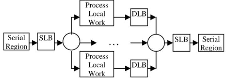
The contiguous and guided scheduling techniques can be categorized as the poorest techniques. The round-robin scheduling technique comes next in the ranking. The αcoefficient for the cost of local work term (c_LW) in equation App.1 implies this selection. Equation App.1 shows the algebraic cost model expression for parallel programs parallelized at with finer granularity level. Theαcoefficient is dependent on how granular the chunk-size is spread across the processors. The finer selection is achieved by the cost of load-balancing term (c_S/DLB). In other words, c_S/DLB represents the synchronization overhead in the parallel program. This term is zero for a serial program. Figure 7 abstracts any parallel program parallelized at finer granularity level in terms of these two major terms. Here, the main assumption for this cost model is that the time spent in the parallel region is much greater than the time spent in the serial region andB<<n/p, both of which hold for our formulation.

Figure 7. Generic parallel program parallelized at finer granularity level

(App.1) c_total=α∗c_LW+c_S/DLB

Since affinity scheduling does an initial scheduling at compile time, it may have less overhead then the dynamic scheduling. A possible partial ranking is shown in Figure 8.a. The worst point in this space is at the upper right-hand corner where synchronization cost (i.e.c_S/DLB) is too high and the load-imbalance (i.e.c_LW) reaches the most non-uniform state. The best point is at the lower left-hand corner where synchronization cost is the lowest and the load-imbalance is almost zero, which is hypothetical. The real scenarios lie between these two extremes. Thus, the decision tree in Figure8.b

Serial Region SLB Process Local Work Process Local Work

…

summarizes a possible total ranking of the load-balancing techniques used in this study.

(a) (b) Figure 8. a) Partial Ranking and b) Total Ranking of load-balancing

techniques best worst Load imbalance Synchronization cost Round-robin Contiguous Affinity Dynamic Guided round- robin contiguous guided affinity dynamic Load Balance medium poor Synchr. cost high low good