MNRAS471,1088–1106 (2017) doi:10.1093/mnras/stx1647
Advance Access publication 2017 June 30
The Cluster-EAGLE project: global properties of simulated clusters
with resolved galaxies
David J. Barnes,
1‹Scott T. Kay,
1Yannick M. Bah´e,
2Claudio Dalla Vecchia,
3,4Ian G. McCarthy,
5Joop Schaye,
6Richard G. Bower,
7Adrian Jenkins,
7Peter A. Thomas,
8Matthieu Schaller,
7Robert A. Crain,
5Tom Theuns
7and Simon D. M. White
21Jodrell Bank Centre for Astrophysics, School of Physics and Astronomy, The University of Manchester, Manchester M13 9PL, UK 2Max-Planck-Institut f¨ur Astrophysik, Karl-Schwarzschild Str. 1, D-85748 Garching, Germany
3Instituto de Astrof´ısica de Canarias, C/ V´ıa L´actea s/n, E-38205 La Laguna, Tenerife, Spain
4Departamento de Astrof´ısica, Universidad de La Laguna, Av. del Astrof´ısico Francisco S´anchez s/n, E-38206 La Laguna, Tenerife, Spain 5Astrophysics Research Institute, Liverpool John Moores University, 146 Brownlow Hill, Liverpool L3 5RF, UK
6Leiden Observatory, Leiden University, PO Box 9513, NL-2300 RA Leiden, the Netherlands
7Institute for Computational Cosmology, Department of Physics, University of Durham, South Road, Durham DH1 3LE, UK 8Astronomy Centre, University of Sussex, Falmer, Brighton BN1 9QH, UK
Accepted 2017 June 28. Received 2017 June 6; in original form 2017 March 31
A B S T R A C T
We introduce the Cluster-EAGLE (C-EAGLE) simulation project, a set of cosmological
hydro-dynamical zoom simulations of the formation of 30 galaxy clusters in the mass range of 1014<M200/M<1015.4that incorporates theHydrangeasample of Bah´e et al. (2017). The
simulations adopt the state-of-the-artEAGLEgalaxy formation model, with a gas particle mass
of 1.8×10⁶M and physical softening length of 0.7 kpc. In this paper, we introduce the
sample and present the low-redshift global properties of the clusters. We calculate the X-ray properties in a manner consistent with observational techniques, demonstrating the bias and scatter introduced by using estimated masses. We find the total stellar content and black hole masses of the clusters to be in good agreement with the observed relations. However, the clusters are too gas rich, suggesting that the active galactic nucleus (AGN) feedback model is not efficient enough at expelling gas from the high-redshift progenitors of the clusters. The X-ray properties, such as the spectroscopic temperature and the soft-band luminosity, and the Sunyaev–Zel’dovich properties are in reasonable agreement with the observed relations. However, the clusters have too high central temperatures and larger-than-observed entropy cores, which is likely driven by the AGN feedback after the cluster core has formed. The total metal content and its distribution throughout the intracluster medium are a good match to the observations.
Key words: hydrodynamics – methods: numerical – galaxies: clusters: general – galaxies: clusters: intracluster medium – X-rays: galaxies: clusters.
1 I N T R O D U C T I O N
The observable properties of galaxy clusters emerge from the com-plex interplay of astrophysical processes and gravity acting on hier-archically increasing scales. Cluster formation is a process that has an enormous dynamic range, as clusters collapse from fluctuations with a comoving scale length of tens of Mpc, but have observ-able properties that are shaped by highly energetic astrophysical
E-mail:[email protected]
processes acting on subparsec scales (see Voit2005; Allen, Evrard & Mantz2011; Kravtsov & Borgani2012, for recent reviews). The interaction of processes acting on very different scales makes cluster formation a highly non-linear process. However, the combination of scales and processes make galaxy clusters a unique environ-ment where we can observe not only the material that participated in galaxy formation but also the material that did not. Therefore, clusters allow the simultaneous study of fundamental cosmologi-cal parameters, gravity, hydrodynamicosmologi-cal effects, chemicosmologi-cal element synthesis and the interaction of relativistic jets with the cluster environment.
C
Although significant progress can be made with semi-analytic prescriptions (Bower, McCarthy & Benson 2008; Somerville et al.2008; Guo et al.2011; Bower, Benson & Crain2012), hy-drodynamical simulations are the only method that can capture the effects of physical processes during cluster formation and predict the resulting observable consequences self-consistently. Although unable to capture the full dynamic range due to limited computa-tional resources, there has been significant progress in the modelling of cluster formation and the physical processes that occur below the resolution scale of the simulation, so-called subgrid models. The formation of the baryonic component of clusters has been well studied (e.g. Eke, Navarro & Frenk1998; Kay et al.2004; Crain et al.2007; Nagai, Kravtsov & Vikhlinin2007b; Sijacki et al.2007; Dubois et al.2010; Short et al.2010; Young et al.2011; Battaglia et al.2012; Gupta et al.2016), including the importance of feedback from active galactic nuclei (AGNs) and its effect on the baryonic content of clusters (e.g. Puchwein, Sijacki & Springel2008; Fab-jan et al.2010; McCarthy et al.2010; Martizzi et al.2016). These developments have led to several independent groups simulating samples of clusters that are to varying degrees realistic (Le Brun et al.2014; Pike et al.2014; Planelles et al.2014; Rasia et al.2015; Hahn et al.2017), i.e. their observable properties, such as X-ray lu-minosity and spectroscopic temperature, are a good match to those of observed clusters. The understanding that subgrid models should be calibrated against carefully selected observable relations has re-sulted in simulations that simultaneously reproduce a host of stellar, gas and halo properties (McCarthy et al.2017), even to high redshift (Barnes et al.2017). One limitation of previous cluster formation simulation work is that it only achieved a modest resolution, typ-ically with a gas particle mass ofmgas ∼109M[for smoothed particle hydrodynamic (SPH) simulations] and a spatial resolution of∼5 kpc. This limits the ability to resolve the structures in the intracluster medium (ICM), to examine the interactions between energetic astrophysical processes and the ICM, to capture the for-mation and evolution of the cluster galaxy population, and to resolve the growth histories of the black holes (BHs).
At the same time, there has been significant progress in the the-oretical modelling of galaxy formation in representative volumes. Improved resolution and the development and calibration of effi-cient subgrid prescriptions for feedback processes have led to a step change in the realism of galaxy formation models (Vogels-berger et al.2014; Crain et al. 2015; Schaye et al. 2015; Dav´e, Thompson & Hopkins2016; Tremmel et al.2017). For example, theEAGLEsimulation suite (Schaye et al.2015; Crain et al.2015) was calibrated against the observed galaxy stellar mass function, the field galaxy size–mass relation and the BH mass–stellar mass relation at low redshift. Following this, the model then yields broad agree-ment with, among other things, the observed evolution of galaxy star formation rates (Furlong et al.2015), the evolution of galaxy sizes (Furlong et al.2017), their molecular and atomic hydrogen content (Lagos et al.2015; Bah´e et al.2016; Crain et al. 2017), their observed colour distribution (Trayford et al.2015), and the growth of BHs and their link to the star formation and growth of galaxies (Rosas-Guevara et al.2016; Bower et al.2017; McAlpine et al.2017). However, the resolution required and complexity of the subgrid models make these simulations computationally expen-sive, limiting their volume to periodic cubes with a side length of ∼100 Mpc or less. Although a volume of this size will contain many galaxy groups (M200=1013–1014M1), rich galaxy clusters (M200
1We defineM200as the mass enclosed within a sphere of radiusr200whose mean density is 200 times the critical density of the Universe.
≥1015M
) are very rare objects and a volume of this size is highly unlikely to contain even one. Therefore, it is difficult to assess the ability of these calibrated models to produce realistic large-scale structures, such as galaxy clusters, and to test whether they cor-rectly capture galaxy formation in the full range of environments.
Motivated by the limitations of existing cluster and galaxy for-mation simulations, we introduce the Virgo consortium’s Cluster-EAGLE (C-Cluster-EAGLE) project. The project consists of zoom simulations of the formation of 30 galaxy clusters that are evenly spaced in the mass range of 1014–1015.4M
, probing environments that are not present in the original periodicEAGLEvolumes presented by Schaye et al. (2015), henceforthS15, and Crain et al. (2015). They are per-formed with theEAGLEgalaxy formation model (AGNdT9 calibra-tion) and adopt the same mass resolution (mgas=1.81×10⁶M) and physical spatial resolution (=0.7 kpc) as the largest periodic volume of theEAGLEsuite (Ref-L100N1504). The resolution of the simulations allows us to resolve the formation of cluster galaxies and their co-evolution with the ICM, the interactions between the cluster galaxies and the ICM, the formation of structures within the ICM, and how energetic astrophysical processes shape the ICM. As the hot halo typically extends to several virial radii, the zoom regions extend to at least five times the virial radius of each object to include the large-scale structure around them. TheHydrangea sam-ple (Bah´e et al.2017), designed to study the evolution of galaxies as their environment transitions from isolated field to dense clus-ter, extends the zoom region to 10 virial radii for 24 of 30C-EAGLE clusters.
In this paper, we present the global properties and hot gas profiles of the simulated clusters at low redshift and compare to observations in order to examine the ability of a model calibrated for galaxy formation to produce realistic galaxy clusters. In a companion paper (Bah´e et al.2017), the properties of the cluster galaxy population are presented and theHydrangeasample is used to study the impact of the cluster environment on the galaxy stellar mass function. The predicted galaxy luminosity functions of the clusters will be presented in Dalla Vecchia et al. (in preparation), including results for higher-resolution runs of a subset of the clusters. The rest of this paper is structured as follows. In Section 2, we present the sample selection, a brief overview of the EAGLE model and the method adopted for computing global properties in a manner consistent with observational techniques, which enables a fairer comparison to observational data. We then compare the global properties of the sample to observational data in Section 3 and examine the hot gas profiles of the sample in Section 4. Finally, we discuss our results in Section 5 and present a summary of the main findings in Section 6.
2 N U M E R I C A L M E T H O D
This section provides an overview of the cluster sample selection, the model used to resimulate them and how the observable prop-erties were calculated in a manner consistent with observational approaches.
2.1 Sample selection
1090
D. J. Barnes et al.
a cubic periodic volume with a side length of 3.2 Gpc, which is large enough to contain the rarest and most massive haloes expected to form in aCDM cosmology. Atz=0, it contains 185 150 haloes withM200>1014Mand 1701 haloes withM200>1015M. The sample was selected by first binning all haloes into 10 evenly spaced log mass bins in the range of 14.0≤log10(M200/M)≤15.4. We did this to ensure that we evenly sampled the chosen mass range, otherwise we would have been biased towards lower masses by the steep slope of the mass function. To ensure that our selected objects would be at the centre of the peak in the local density structure and the focus of our computational resources, we removed objects from the selection bins who had a more massive neighbour within a sphere whose radius was the larger value of either 30 Mpc or 20r200. We then randomly picked three haloes from each mass bin to yield a sample of 30 objects, which are listed in Appendix A.
We used the zoom simulation technique (Katz & White1993; Tormen, Bouchet & White1997) to resimulate our chosen sample at higher resolution. The Lagrangian region of every cluster was selected so that its volume was devoid of lower resolution particles beyond a cluster-centric radius of at least 5r200atz=0. Addition-ally, the Lagrangian regions of theHydrangeasample were defined such that they were devoid of lower resolution particles beyond a cluster-centric radius of 10r200, enabling studies of galaxy evo-lution as the environment transitions from isolated field to dense cluster. Atz=127, the initial glass-like particle configuration of the high-resolution regions was deformed according to the second-order Lagrangian perturbation theory using the method of Jenkins (2010) andPANPHASIA(Jenkins2013), a multiscale Gaussian white noise field that is publicly available.2 We assumed a flatcold dark matter (CDM) cosmology based on thePlanck2013 results combined with baryonic acoustic oscillations,WMAPpolarization and high-multipole moments experiments (Planck Collaboration et al. 2014). The cosmological parameters were b = 0.04825,
m=0.307,=0.693,h≡H0/(100 km s−1Mpc−1)=0.6777,
σ8=0.8288,ns=0.9611 andY=0.248. The resolution of the La-grangian regions was increased to match the resolution of theEAGLE 100 Mpc simulation (Ref-L100N1504). The dark matter particles each had a mass ofmDM=9.7×10⁶Mand the gas particles each had an initial mass ofmgas =1.8×10⁶M(note noh−1). The proper gravitational softening length for the high-resolution region was set to 2.66 comoving kpc forz>2.8, and then kept fixed at 0.70 physical kpc forz<2.8. The minimum smoothing length of the SPH kernel was set to a 10th of the gravitational softening scale.
2.2 The eagle model
We use the EAGLE model to resimulate our selected sample. The EAGLEsubgrid model is based on the model developed for theOWLS (Schaye et al. 2010) project and also used for theGIMIC (Crain et al.2009) andCOSMO-OWLS(Le Brun et al.2014) models. The sub-grid model, the calibration of its free parameters and its numerical convergence are described in detail inS15and Crain et al. (2015). The code is a heavily modified version of theN-body Tree-PM SPH codeP-GADGET-3, which was last described in Springel (2005). The hydrodynamics algorithms are collectively known as ‘ANARCHY’ [see Dalla Vecchia in preparation), appendix A ofS15and Schaller et al. (2015)] and consists of an implementation of the pressure-entropy SPH formalism derived by Hopkins (2013), an artificial viscosity
2The phase descriptor of the parent volume is given in Appendix A and in table B1 ofS15.
switch (Cullen & Dehnen2010), an artificial conductivity switch similar to that of Price (2008), theC2smoothing kernel with 58 neighbours (Wendland1995) and the time-step limiter of Durier & Dalla Vecchia (2012). The subgrid model includes radiative cool-ing, star formation, stellar evolution, feedback due to stellar winds and supernovae, and the seeding, growth and feedback from BHs. We now briefly describe the subgrid model in more detail.
Net cooling rates are calculated on an element-by-element basis following Wiersma, Schaye & Smith (2009a), under the assumption of an optically thin gas in ionization equilibrium, the presence of the cosmic microwave background and an evolving ultraviolet/X-ray background (Haardt & Madau2001) from galaxies and quasars. This is done by interpolation tables, computed usingCLOUDY ver-sion 07.02 (Ferland et al. 1998), that are a function of density, temperature and redshift for the 11 elements that were found to be important. During reionization, 2 eV per proton mass is injected to account for enhanced photoheating rates. For hydrogen this occurs instantaneously atz=11.5 and for helium this additional heating is Gaussian distributed in redshift, centred onz=3.5 with a width
σ(z)= 0.5. The latter ensures that the observed thermal history of the intergalactic gas is broadly reproduced (Schaye et al.2000; Wiersma et al.2009b).
Star formation is modelled stochastically in a way that, by construction, reproduces the observed Kennicutt–Schmidt relation, as cosmological simulations lack the resolution and physics to properly model the cold interstellar gas phase. It is implemented as a pressure-law (Schaye & Dalla Vecchia 2008), subject to a metallicity-dependent density threshold (Schaye2004). Gas par-ticles whose density exceeds nH(Z) = 10−1cm−3(Z/0.002)−0.64, whereZis the gas metallicity, are eligible to form stars. Lacking the resolution and physics to model the cold gas phase, a temperature floor,Teos(ρg), is imposed that corresponds to the equation of state
Peos∝ρg4/3, normalized toTeos=8×10³K atnH=10−1cm−3. This helps to prevent spurious fragmentation. Stellar evolution and the resulting chemical enrichment is based upon Wiersma et al. (2009b). Star particles are treated as simple stellar populations with a mass range of 0.1–100 M and a Chabrier (2003) initial mass function. Mass loss and the release of 11 chemical elements due to winds from massive stars, asymptotic giant branch stars and type Ia and type II supernovae are tracked. Feedback from star formation is implemented using the stochastic thermal model of Dalla Vecchia & Schaye (2012). The energy injected heats a particle by a fixed temperature increment,T=107.5K, to prevent spurious numer-ical losses. The energy per unit of stellar mass formed, which sets the probability of heating events, depends on the local gas density and metallicity and is calibrated to ensure that the galaxy stellar mass function and galaxy size–mass relation are a good match to the observed relations atz=0.1 (Crain et al.2015).
Feedback from supermassive BHs is a critical component of structure formation simulations, shaping the bright end of the galaxy luminosity function (e.g. Bower et al.2006; Croton et al.2006), the gas content of clusters (e.g. Puchwein et al.2008; Fabjan et al.2010; McCarthy et al.2010) and preventing the onset of the overcooling problem (McCarthy et al.2011). The prescription for the seeding, growth and feedback from BHs is based on Springel, Di Matteo & Hernquist (2005) with modifications from Booth & Schaye (2009) and Rosas-Guevara et al. (2015). Seed BHs are placed in the centre of every halo with a total mass greater than 1010M
with other BHs or via the accretion of gas. The gas accretion rate is Eddington limited and depends on the mass of the BH, the local gas density and temperature, and the relative velocity and angular momentum of the gas compared to the BH:
˙
maccr=m˙Bondi×min(Cvisc−1(cs/Vφ)3,1), (1) where ˙mBondi is the Bondi & Hoyle (1944) spherically symmetric accretion rate,csis the sound speed of the gas andVφis the rotation speed of the gas around the BH (see equation 16 of Rosas-Guevara et al.2015).Cviscis a free parameter for the effective viscosity of the subgrid accretion disc/torus and larger values correspond to a lower kinetic viscosity, which delays the growth of BHs and the onset of feedback events. We note that the results are remarkably insensi-tive to a non-zero value ofCvisc (Bower et al.2017). The growth of the BH is then given by ˙mBH=(1−r) ˙maccr, wherer =0.1 is the radiative efficiency. The accretion rate is not multiplied by a constant or density-dependent factor as is common to many pre-vious studies (Springel et al.2005; Booth & Schaye2009), as at the resolution ofEAGLE, we resolve sufficiently high-gas densities and the accretion rate is sufficient for the BH seeds to grow by Bondi–Hoyle accretion.
AGN feedback is implemented in a similar way to stellar feed-back, whereby thermal energy is injected stochastically. Energy is injected at a rate offrm˙accrc2, wherecis the speed of light and
f=0.15 is the fraction of energy that couples to the gas. Booth & Schaye (2009) found that forOWLS, this value yielded agreement with the observed BH masses andS15found that the same holds forEAGLE. In order to prevent spurious numerical losses and enable the feedback to do work on the gas before the injected energy is radiated, the BH stores accretion energy until it reaches a critical energy, at which point it has enough energy to heatnheatparticles by a temperatureT. In theEAGLEmodel,nheat=1. In the pressure– entropy SPH formalism used inEAGLE, the weighted density and entropic function are coupled (S15, see appendix A1.1). For large changes in internal energy, such as AGN feedback events, the iter-ative scheme used to adjust the density and entropic function fails to adequately conserve energy if many particles are heated simul-taneously. This leads to a violation of energy conservation. The probability of heating a neighbour particle is given by
P = EBH
AGNNngbmgas
, (2)
whereEBHis the energy reservoir of the BH,AGN is the spe-cific energy associated with heating a particle byT,Nngbis the number of gas neighbours and mgasis their average mass. AsEBH increases the probability of heating many neighbours increases and a violation of energy conservation becomes more likely. To prevent this, the probability is capped at a value ofPAGN=0.3, a value that was chosen following testing of the iterative scheme. If the unused energy remains above the critical threshold for a feedback event then the time step of the BH is shortened and the energy spread out over successive steps.
S15 present three calibrated models (REF, AGNdT9 and Re-cal) that produce a similarly good match to the observed galaxy stellar mass function and galaxy mass–size relation. As we are running at standardEAGLEresolution, we ignore the Recal model, which is relevant for simulations with 8×higher mass resolution. From figs 15 and 16 ofS15, it is clear that the AGNdT9 model provides a better match to the observed gas fraction-total mass and X-ray luminosity–temperature relations of low-mass groups (M500<1013.5M). Therefore, we select the AGNdT9 model as our fiducial model for theC-EAGLEproject; the free parameters of
Table 1. Values of the AGN feedback free parameters of the AGNdT9 model, used for theC-EAGLEsimulations and the 50 MpcEAGLEvolume, and the REF model, used for the 100 MpcEAGLEvolume.
Model nheat Cvisc T(K)
AGNdT9 1 2π×102 109
REF 1 2π 108.5
the AGN feedback for this model and for the REF model are given in Table1. This model was calibrated in a 50 Mpc cubic volume to produce good agreement between simulated and observed galaxies. Furthermore, Crain et al. (2015) showed that the simulated BH– stellar mass relation and galaxy mass–size relation are sensitive to the feedback parameters used. We do not recalibrate the model to cluster scale objects and instead choose to retain the match to the observed galaxy properties. Therefore, the properties of the ICM for theC-EAGLEclusters are a prediction of a model that produces reasonably realistic field galaxies.
2.3 Calculating X-ray and Sunyaev–Zel’dovich properties
Inhomogeneities in the hot gas, e.g. the presence of multitemper-ature structures, can significantly bias the ICM properties inferred from X-ray observations (e.g. Nagai, Vikhlinin & Kravtsov2007a; Khedekar et al.2013). Therefore, when comparing simulations to observations it is vital to make a like-with-like comparison and com-pute properties from simulated clusters in a manner more consistent with observational techniques.
Following Le Brun et al. (2014), we produce mock X-ray spec-tra for each cluster by first computing a rest-frame X-ray spectrum in the 0.05–100.0 keV band for each gas particle, using their indi-vidual density, temperature and SPH-smoothed metallicity. We use the Astrophysical Plasma Emission Code (APEC; Smith et al.2001) via the PYATOMDBmodule with atomic data from ATOMDBv3.0.3 (last described in Foster et al. 2012). For each of the 11 el-ements, we calculate an individual spectrum, ignoring particles with a temperature less than 105K, as they will have negligible X-ray emission.
Particles are then binned, in three-dimensional (3D), into 25 logarithmically spaced radial bins centred on the potential mini-mum and the spectra are summed for each bin. The binned spec-tra are scaled by the relative abundance of the heavy elements, as the fiducial spectra assume solar abundances specified by An-ders & Grevesse (1989). The energy resolution of a spectrum is 150 eV between 0.05 and 10.0 keV and we use a further 10 logarithmically spaced bins between 10.0 and 100.0 keV. A sin-gle temperature, fixed metallicityAPECmodel is then fitted to the spectrum in the range of 0.5 and 10.0 keV, for each radial bin, to derive an estimate of the density, temperature and metallicity. During the fit we multiply the spectrum by the effective area of
Chandrafor each energy bin to provide a closer match to typical X-ray observations.
We then perform a hydrostatic analysis of each cluster us-ing the X-ray-derived density and temperature profiles. We fit the density and temperature models proposed by Vikhlinin et al. (2006) to obtain a hydrostatic mass profile. We then estimate var-ious cluster masses and radii, such as M500 and r500, from the hydrostatic analysis. We calculate properties, such as gas mass,
1092
D. J. Barnes et al.
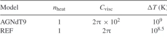
Figure 1. Image of CE-5 and its environment atz=0.1, resimulated using theEAGLEAGNdT9 model. The colour map shows the gas, with the intensity depicting the density of the gas and the colour depicting the temperature of the gas. Stellar particles are shown by the white points and the dashed yellow circle denotesr200. The inset colour map shows the X-ray surface brightness from a cubic region of 2r500, centred on the cluster’s centre of potential.
properties of the particles that fall within the estimated X-ray aper-tures. A core-excised quantity is calculated by summing particles that fall in the radial range of 0.15–1.0 of the specified aperture. To calculate X-ray luminosities, we integrate the spectra of parti-cles that fall within the aperture in the required energy band; for example, the soft band luminosities are calculated between 0.5 and 2.0 keV. To estimate a spectroscopic X-ray temperature within an aperture, we sum the spectra of all particles that fall within it and then fit a single temperatureAPECmodel to the combined spectrum. All quantities that are derived in this way are labelled as ‘spec’ quantities. In Appendix A, we also provide the values of estimated quantities for each cluster atz=0.1.
In Fig. 1, we show an image of the gas and stars for CE-5 at z = 0.1. The resolution and subgrid physics of the EAGLE model enable the simulation to capture the formation of galax-ies in the dense cluster environment and the surrounding fila-mentary structures. The inset panel shows soft band (0.5–2.0 keV) X-ray surface brightness within 2r500of the potential minimum of the cluster.
3 G L O B A L P R O P E RT I E S
In this section, we compare the global properties of theC-EAGLE sample atz= 0.1 with low-redshift (z≤0.25) observations. We also plot the groups and clusters from the periodic volumes of the EAGLEsimulations. We label groups and clusters from the 100 Mpc volume run with theEAGLEreference model as ‘REF’ and those from the 50 Mpc volume run with the AGNdT9 model as ‘AGNdT9’. To ensure a fair comparison with observational data, we use quanti-ties estimated via the mock X-ray analysis pipeline. However, we stress that estimated masses assume that the cluster is in hydrostatic equilibrium and that the X-ray-estimated density and temperature profiles are good approximations of the true profiles. First, we test this assumption.
3.1 Bias and scatter of estimated masses
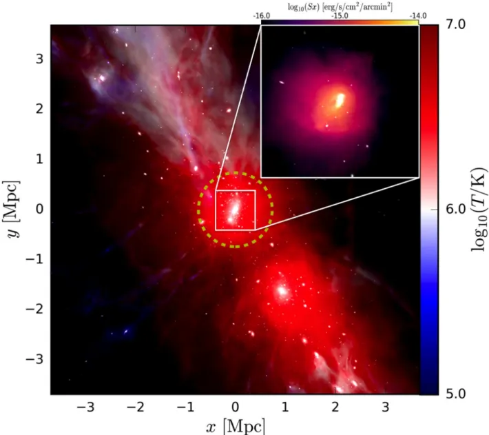
Figure 2. Ratio of estimated to true mass as a function of true mass atz=0.1 for theC-EAGLEclusters (red squares), as well as the groups and clusters from the EAGLEREF (grey circles) and AGNdT9 models (purple diamonds). The left-hand panel shows hydrostatic mass estimates, calculated by fitting Vikhlinin et al. (2006) models to the true profiles, while the right-hand panel shows X-ray spectroscopic mass estimates, calculated by fitting Vikhlinin et al. (2006) models to profiles estimated from the mock X-ray pipeline. Clusters that are defined as relaxed (unrelaxed) are shown by the filled (open) points. The dashed black line indicates no bias.
estimatedM500over M500,true as a function ofM500,true, where the ‘true’M500values are calculated via summation of particle masses that fall within the truer500. To separate the effects of assuming hy-drostatic equilibrium and estimating the profiles in an observational manner via the X-ray pipeline, we also fit the Vikhlinin et al. (2006) models to the true density and temperature profiles and label any quantity computed in this manner as ‘hse’.
Fig.2shows the scatter and bias introduced by estimating the mass for theC-EAGLE clusters as well as the REF and AGNdT9 groups and clusters. The assumption of hydrostatic equilibrium in-troduces a median biasbhse=0.16±0.04 for theC-EAGLEclusters, wherebhse=1−M500,hse/M500,trueand the error is calculated by bootstrap resampling the data 10 000 times. The assumption of hy-drostatic equilibrium introduces a similar bias in the REF and AG-NdT9 groups and clusters, which yield values ofbhse=0.14±0.02 andbhse =0.21±0.06, respectively. We find that the bias intro-duced by assuming hydrostatic equilibrium is independent of mass. This is consistent with previous simulation work that has anal-ysed true profiles (Nelson et al.2014; Biffi et al.2016; Henson et al.2017). For theC-EAGLEclusters, the profiles derived from the mock X-ray analysis produce a slightly larger bias with a median valuebspec=0.22±0.04. Combined with the REF and AGNdT9 groups and clusters, it is clear that using the X-ray derived profiles increases the scatter in the estimated masses, withC-EAGLEyielding rms values ofσhse=0.16 andσspec=0.18 for the hse and spec values, respectively. Additionally, the spectroscopic bias appears to become mildly mass dependent for the mock X-ray pipeline mass estimates. This is consistent with previous simulation work that has made use of mock X-ray pipelines; Le Brun et al. (2014) saw an increase in scatter for low-mass (<1013M
) groups and a median bias consistent with zero and Henson et al. (2017) found that the bias from mock X-ray pipelines showed a mild mass dependence.
Several of the C-EAGLE clusters have mass estimates that are more than 30 per cent discrepant from their true mass. To better
understand the impact of the dynamical state of a cluster on the estimation of its mass, we classify each object as relaxed or un-relaxed. Theoretically, there are many ways of defining whether a cluster is relaxed (see Neto et al.2007; Duffy et al.2008; Klypin, Trujillo-Gomez & Primack2011; Dutton & Macci`o2014; Klypin et al.2016). In this work, we define a cluster as being relaxed if
Ekin,500,spec/Etherm,500,spec<0.1,
whereEkin,500,specis the sum of the kinetic energy of the gas parti-cles, with the bulk motion of the cluster removed, insider500and
Etherm, 500, specis the sum of the thermal energy of the gas particles withinr500. In all figures, we denote relaxed (unrelaxed) clusters by solid (open) points. Using this criterion, 11 of the 30C-EAGLE clusters are defined as relaxed.
Selecting only relaxed (unrelaxed) C-EAGLE clusters, we mea-sure median mass biases bhse = 0.14± 0.02 (0.19 ± 0.03) and
bspec=0.16±0.03 (0.26±0.04). Thus, the mass estimates of re-laxed clusters show a small decrease in the level of bias compared to the full sample, but the scatter in the mass estimate reduces sig-nificantly toσhse=0.06 andσspec=0.06. The bias of unrelaxed clusters increases slightly and the scatter about the median value increases toσhse=0.23 andσspec =0.21. We see a similar trend for the REF and AGNdT9 groups and clusters. We also find that all C-EAGLEclusters with a mass estimate that is more than 30 per cent discrepant from its true mass haveEkin,500,spec/Etherm,500,spec>0.1, demonstrating the impact of the dynamical state of the cluster on its estimated mass.
3.2 Gas, stellar and BH masses
1094
D. J. Barnes et al.
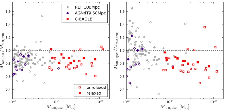
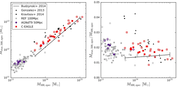
Figure 3. Integrated stellar mass (left-hand panel) and stellar fraction (right-hand panel) withinr500,specas a function of estimated total mass atz=0.1 for theC-EAGLEclusters and the REF and AGNdT9 groups and clusters. Marker styles are the same as in Fig.2. The black triangles and hexagons show the observational data from Gonzalez et al. (2013) and Kravtsov et al. (2014), respectively, and the black line with error bars shows the best-fitting result from Budzynski et al. (2014) from stacking SDSS images.
Hahn et al.2017; McCarthy et al.2017). Therefore, the gas, stellar and BH masses of theC-EAGLEclusters provide a test, orthogonal to usual tests of galaxy formation, of the feedback model and whether calibration on against galaxy properties alone leads to a reasonably realistic ICM.
3.2.1 Stellar mass
We plot the integrated stellar mass and stellar fraction withinr500,spec as a function of the estimated total mass atz = 0.1 in the left-hand and right-left-hand panels of Fig. 3, respectively. To ensure a fair comparison, we only compare theC-EAGLE, REF and AGNdT9 samples against observations where the mass of the system has been estimated via high-quality X-ray observations. The stellar mass-total mass relation withinr500,true is shown in fig. 4 of Bah´e et al. (2017). All of the observations and the simulations include the intracluster light in the stellar mass estimate and assume a Chabrier (2003) initial mass function. First, we note that the observations do not appear to be consistent with each other. The results of Budzynski et al. (2014) have a lower normalization compared to the results of Kravtsov, Vikhlinin & Meshscheryakov (2014) and Gonzalez et al. (2013) atM500=1014M, and the stellar fraction of Budzynski et al. (2014) increases slightly with total mass while Kravtsov et al. (2014) and Gonzalez et al. (2013) show a strongly decreasing stellar fraction with increasing total mass. This is most likely due to the different selection criteria and methods used in the observations.
TheC-EAGLEclusters provide a consistent extension into the high-mass regime of the original periodic volumes. Estimating the clus-ter’s mass from the X-ray hydrostatic analysis leads to an increased scatter about the relation compared to using the true mass, increasing fromσlog10,true=0.07 toσlog10,spec=0.10.3If only relaxed systems
3We measure the scatter by fitting a power law to the stellar mass–total mass relation for the fullC-EAGLEsample, the relaxed subset and the unrelaxed
are considered the scatter reduces substantially toσlog10,spec=0.03. Taken together with groups and clusters from the periodic volumes, theC-EAGLEclusters show reasonable agreement with the observa-tions. They reproduce the trend of the best-fitting stellar mass–total mass relation of Budzynski et al. (2014), but have a slightly higher normalization. In contrast, they reproduce the normalization of the Gonzalez et al. (2013) and Kravtsov et al. (2014) observations and are within the intrinsic scatter, but the trend with total mass is dif-ferent. This is better seen in the stellar fraction–total mass relation, where the results of Gonzalez et al. (2013) and Kravtsov et al. (2014) show an increase in stellar fraction for lower mass objects, while theC-EAGLE clusters combined with the REF and AGNdT9 objects produce a roughly constant stellar mass fraction over two decades in mass. Overall,≈2 per cent of the total mass of the sim-ulated groups and clusters consists of stars. This is consistent with previous numerical work, which has shown that the stars make up a few per cent of the cluster mass and the trend with mass is relatively mild (e.g. Planelles et al.2013; Pike et al.2014; Hahn et al.2017). TheEAGLEmodel was calibrated to reproduce the observed galaxy stellar mass function of the field at low redshift, but dense cluster environments were not present in the calibration volumes due to their limited size. The level of agreement between theC-EAGLE clus-ters and the observations is, therefore, reassuring and demonstrates that the galaxy calibrations continue to work in the cluster regime.
3.2.2 BH masses
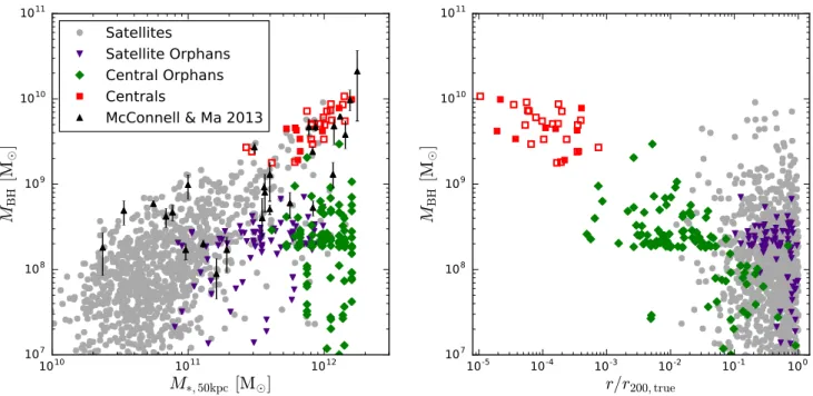
We examine the properties of the supermassive BHs that form in the C-EAGLEclusters in Fig.4. In the left-hand panel, we plot BH mass as a function of stellar mass, calculated within a 3D aperture of radius 50 kpc, for those BHs with a mass>107M
that fall withinr200,true.
Figure 4. BH mass as a function of stellar mass within a 3D 50 kpc aperture (left-hand panel) and cluster-centric radius (right panel) for those BHs that fall withinr200of aC-EAGLEcluster atz=0.1. The population is divided between centrals (red squares), satellites (grey circles), orphan BHs associated with the main halo (green diamonds) and orphans associated with satellites (purple triangles). For the centrals, we denote whether the cluster is relaxed (unrelaxed) by filled (open) marker style. The black triangles show the observations of McConnell & Ma (2013) for early type galaxies.
In total, theC-EAGLEsample contains 1358 BHs withinr200,true. The aperture radius is a choice and we select 50 kpc as it mimics common observational choices. We decompose the bound population into centrals (those bound to the main halo) and satellites (those bound to subhaloes) as determined by theSUBFIND algorithm (Springel et al.2001; Dolag et al.2009). We find that 90 per cent of all BHs are defined as satellites. The central and satellite BHs form a continuous population on the BH mass–stellar mass relation. We compare the simulation relation to the observed early type galaxies from the compilation of McConnell & Ma (2013). We find good agreement with the observed relation, with theC-EAGLEclusters reproducing both the observed trend and normalization. As demonstrated in Booth & Schaye (2010), the normalization of the BH mass–stellar mass relation is set by the feedback efficiency and the chosen value off=0.15 has been shown to work in low-resolution simulations of galaxies (Booth & Schaye2009), clusters (Le Brun et al.2014) and in theEAGLEperiodic volumes (S15).
Additionally, we define orphan BHs as those that are bound to either the main halo or a subhalo, but are not the most massive BH associated with it. We find that≈15 per cent of BHs within
r200,trueare classified as orphans. We further classify the orphans as being associated either with the main halo or subhaloes and find around 50 per cent of the orphans are linked to the main halo. The number of orphans increases strongly with cluster mass and only subhaloes with a stellar mass>1011M
contain orphans. TheEAGLEmodel allows BHs whose mass exceeds 100mgas to be-come dynamically independent and limits the distance that BHs less massive than this limit can drift towards the potential minimum at each time step. Therefore, when two haloes merge their BHs do not necessarily also instantaneously merge. In the right-hand panel of Fig.4, we plot BH mass as a function ofr/r200,true. The cen-tral BHs all lie within 0.1 per cent ofr200,true from the potential minimum, even though they are all dynamically independent. No satellite BH is closer than 1 per cent ofr200,true. We find that 43
orphans lie within 1 per cent ofr200,true, which equates to a distance of 10–20 kpc from the potential minimum. Therefore, theC-EAGLE simulations predict that there is a population of BHs with a mass
>108M
inside the brightest cluster galaxies (BCGs) that are not the central BH. The orphans, both centrals and satellites, are likely the remnants of previous galaxy mergers, but we note that some may be identified with missed subhaloes as halo finders, such as SUBFIND, have issues indentifying subhaloes in dense backgrounds (Muldrew, Pearce & Power2011). We leave a more detailed exam-ination of the origins and properties of this orphan population to a future study.
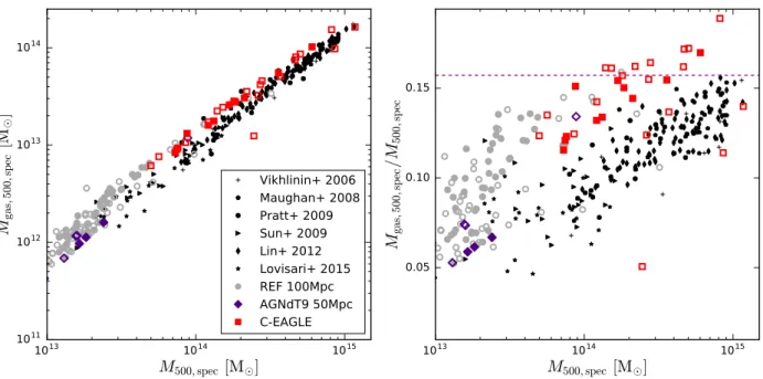
3.2.3 Gas mass
In Fig.5, we plot the gas mass and the gas fraction withinr500,spec as a function of the estimated total mass atz=0.1, in the left-hand and right-hand panels, respectively. Again, we compare against the groups and clusters from the REF and AGNdT9 volumes and obser-vational data. TheC-EAGLEclusters provide a consistent extension to the objects from the periodic volumes. TheC-EAGLEclusters re-produce the observed trend with halo mass, but they are too gas rich and lie along the top of the observed scatter of the gas mass–total mass relation. Although we selected the AGNdT9EAGLEmodel, as it produced a better match to the observed gas fractions of low-mass (<1013.5M
1096
D. J. Barnes et al.
Figure 5. Gas mass as a function of estimated total mass withinr500,specatz=0.1 for theC-EAGLEclusters and the REF and AGNdT9 groups and clusters. Marker styles are the same as in Fig.2. The black pluses, pentagons, circles, right-facing triangles, thin diamonds and stars show the observational data from Vikhlinin et al. (2006), Maughan et al. (2008), Pratt et al. (2009), Sun et al. (2009), Lin et al. (2012) and Lovisari et al. (2015), respectively. The left-hand panel shows the gas mass, whereas the right-hand panel shows gas fractions with the magenta dashed line showing the universal baryon fraction,b/M=0.157.
major merger at z = 0.1, displacing the gas from the potential minimum and leading to an estimated gas mass well below the observed relation.
We also plot the gas fractions as the dynamic range of the gas mass–total mass relation hides some of the discrepancies. As shown inS15, the low-mass (<1013.5M
) groups of the periodic volumes show a significant difference in the gas fraction for the two AGN calibrations, with the increased AGN heating temperature of the AGNdT9 model producing gas fractions that are systematically lower by ≈30 per cent. However, at cluster scales (>1014M
), the runs with different heating temperatures converge towards to the same relation, although we currently suffer from a small sample size. Gas fractions for some of theC-EAGLEclusters appear to be greater than the universal baryon fraction,fb≡b/M=0.157. This is due to using an X-ray estimated mass that is biased low compared to the true mass.
To remove the impact of using an estimated mass, we plot the true gas fraction as a function of M500,true in Fig. 6. The use of true mass significantly reduces the scatter in the relation and all of the simulated clusters are now below the universal fraction, with the most massive clusters reaching≈90 per cent of the universal fraction. However, the simulated clusters and groups above a mass ofM500,spec ≥1013.5Mare still too gas rich. Previous work has shown that the majority of gas expulsion occurs in the progenitors of a halo at high redshift (McCarthy et al.2011). These progeni-tors form at an earlier epoch for more massive objects, when the Universe was denser, making their potentials deeper. The higher-than-observed gas fractions of the groups and clusters suggest that the AGN feedback in the EAGLEmodel is not efficient enough at removing gas from the deeper potentials of the progenitors of mas-sive groups and clusters (>1014M
). This also leads to some overcooling and larger than observed BCGs (see the right-hand panel of fig. 4 of Bah´e et al.2017). We note that the true gas frac-tions for rich clusters (1015M
) appear to be in agreement with the observational data; however, this is clearly no longer a fair comparison.
Figure 6. True gas fraction as a function of true total mass, both within r500,spec, atz=0.1 for theC-EAGLEclusters and the REF and AGNdT9 groups and clusters. Marker styles and observations are the same as in Fig.5.
3.3 X-ray and SZ properties
Having shown that theC-EAGLEclusters have stellar and BH masses in reasonable agreement with the observed relations but are too gas rich, we now examine the X-ray and SZ observable properties at
z=0.1 produced by the mock X-ray pipeline.
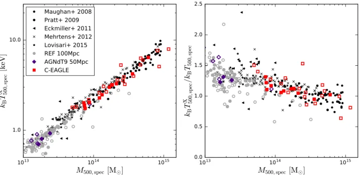
3.3.1 Spectroscopic temperature–total mass
Figure 7. Spectroscopic temperature measured withinr500,specas a function of estimated total mass atz=0.1 for theC-EAGLEclusters and the REF and AGNdT9 groups and clusters. Marker styles are the same as in Fig.2. The black pentagons, circles, left-facing triangles, crosses and stars show observational data from Maughan et al. (2008), Pratt et al. (2009), Eckmiller et al. (2011), Mehrtens et al. (2012) and Lovisari et al. (2015), respectively. The left-hand panel shows the temperature and the right-hand panel shows the temperature normalized by the virial temperature to approximately remove the mass dependence.
the estimated total mass. TheC-EAGLEclusters and the groups and clusters from the REF and AGNdT9 volumes are a good match to the observational data, yielding a linear power-law relation over two decades in mass. TheC-EAGLEsimulations have a scatter of
σlog10=0.06, which is similar to the value of σ = 0.05 found by Eckmiller, Hudson & Reiprich (2011) for theHIFLUGCSsample. Though we calculate properties in a manner consistent with obser-vational techniques, we do not make any attempt to account for observational selection effects. The clusters with the largest scatter are all unrelaxed and these objects may not be selected in X-ray samples due to then2
Hdependence of the emission, which results in a bias towards more relaxed systems.
In the right-hand panel of Fig.7, we have removed the expected mass dependence of the relation that results from hydrostatic equi-librium by dividing each system by its virial temperature, which we calculate as
kBT500,spec≡GM500,specμmp/2r500,spec, (3)
wherekB is the Boltzmann constant,Gis Newton’s gravitational constant,μ=0.59 is the mean molecular weight of the gas and
mp is the proton mass. This allows us to examine the impact of non-gravitational processes, such as cooling and feedback.
The most massiveC-EAGLEclusters have temperature ratios that are close to one, showing that their temperatures are close to the expected virial values. As the mass of the object decreases the temperature increases relative to the virial temperature, being 50 per cent higher than expected for the 1013M
groups in the REF and AGNdT9 samples. This demonstrates that the feedback is able to heat and expel gas more efficiently in lower mass objects. This is consistent with previous simulation work (McCarthy et al.2010; Short et al.2010; Le Brun et al.2014; Planelles et al.2014; Hahn et al.2017). However, in Le Brun et al. (2014), an increase in the AGN heating temperature produced a flatter normalized tempera-ture relation (see the right hand panel in their Fig.2), a difference
that we do not see between the REF and AGNdT9 models. This may be due to resolution as theC-EAGLEclusters achieve a factor 500×better mass resolution, which reduces the energy per AGN feedback event and may reduce the impact of feedback on the cluster properties.
3.3.2 X-ray luminosity–total mass
We plot the soft band (0.5–2.0 keV) X-ray luminosity,L0.5−2.0 keV X,500,spec, withinr500,specas a function of the estimated total mass atz=0.1 in Fig. 8. TheC-EAGLE clusters show reasonable agreement with the observational data, reproducing the observed trend. The nor-malization of the simulated trend is marginally high compared to the observed relation, but still within the scatter, and this is due to the clusters being too gas rich. We note that the merging cluster has a significantly decreased X-ray luminosity for its mass. The completeC-EAGLE sample has a scatter ofσlog10 =0.30, which is larger than the values ofσlog10 =0.17 andσlog10=0.25 found for theREXCESS(Pratt et al.2009) andHIFLUGCS(Lovisari, Reiprich & Schellenberger2015) samples, respectively. However, we stress that we do not attempt to account for selection effects. If we select only relaxed clusters the scatter reduces to σlog10=0.11. TheC-EAGLE clusters are consistent with the clusters of the REF and AGNdT9 samples, with the models producing negligible difference for the X-ray luminosity–mass relation.
1098
D. J. Barnes et al.
Figure 8. Soft band X-ray luminosity withinr500,specas a function of es-timated total mass atz=0.1 for theC-EAGLEclusters and the REF and AGNdT9 groups and clusters. Marker styles are the same as in Fig.2. The black triangles, circles, right-facing triangle, crosses and stars show obser-vational data from Vikhlinin et al. (2009), Pratt et al. (2009), Sun (2012), Mehrtens et al. (2012) and Lovisari et al. (2015), respectively.
We note that the scatter increases for observed low-mass groups, but the scatter in the simulated systems does not. However, this increase in the scatter of observed groups may simply reflect the increasing challenge of measuring the total X-ray emission from low-mass groups, rather than a failure of the simulations to reproduce the scatter of the observed relation.
3.3.3 Metallicity–spectroscopic temperature
In Fig.9, we plot the ‘mass-weighted’ iron abundance withinr500,spec as a function of the spectroscopic temperature atz=0.1. Following Yates, Thomas & Henriques (2017), we estimate the mass-weighted iron abundance via
ZFe,500,spec= r500,spec
0 ZFe,specρgas,specr2dr r500,spec
0 ρgas,specr2dr
, (4)
whereZFe,specandρgas,specare the iron abundance and gas density profiles, respectively, estimated from single temperature fits to the summed particle spectra for 25 3D cluster-centric radial bins and we integrate over those bins that fall withinr500,spec. We compare the simulated samples against consolidated data taken from Yates et al. (2017); see the references therein for more details on the homogenization process and the different samples. If more than one estimate for the observed mass-weighted metallicity or temperature was present for a system, the mean value was taken. We have scaled both the simulated and observational data to the solar abundances of Asplund et al. (2009).
TheC-EAGLEclusters show reasonable agreement with the ob-served metallicity–temperature relation, with a median metallic-ity of Zmed
Fe,500,spec=0.23 Z and an rms scatter of σ = 0.09. The REF and AGNdT9 group clusters are also in agreement with the data, with median metallicities of Zmed
Fe,500,spec=0.26 Z and
Zmed
Fe,500,spec=0.22 Z and scatters ofσ = 0.07 and σ = 0.06, respectively. Overall, the EAGLE model produces a relatively flat
Figure 9. Mass-weighted iron abundance measured withinr500,specas a function of spectroscopic temperature atz=0.1 for theC-EAGLEclusters and the REF and AGNdT9 groups and clusters. Marker styles are the same as in Fig.2. The black triangles show the homogenized observational data from Yates et al. (2017).
mass-weighted metallicity–spectroscopic temperature relation from low-mass groups to rich clusters. Reproducing the global metallic-ities of groups and clusters has been a challenge for previous sim-ulation works, with Martizzi et al. (2016) underpredicting the total metal content of clusters, Planelles et al. (2014) overpredicting the metallicity of more massive clusters and Yates et al. (2017) overpre-dicting the metallicity of groups. Recent observational (McDonald et al.2016; Mantz et al.2017) and numerical (Biffi et al.2017) results demonstrate that the global cluster metallicity shows very little evolution, suggesting that simulations must carefully model the early galaxy formation processes to reproduce the observed cluster metallicity.
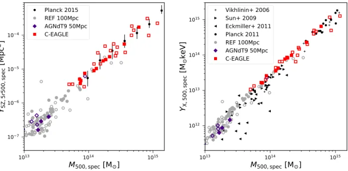
3.3.4 Y-total mass relations
The SZ signal,YSZ, is a measure of the total thermal energy con-tent of the ICM and is thought to be relatively insensitive to the details of the baryonic physics within the cluster volume (da Silva et al.2004; Nagai2006), although see Le Brun et al. (2014). The X-ray analogue of the SZ signal,YX, was first proposed by Kravtsov, Vikhlinin & Nagai (2006) and we define it as the product of the core-excised spectroscopic temperature and the gas mass. The dif-ference between the two quantities is thatYSZis dependent on the mass-weighted temperature, whereasYXis dependent on the core-excised spectroscopic temperature. We plotYSZ within 5r500,spec and YX within r500,spec as a function of the estimated total mass withinr500,spec atz= 0.1 in Fig.10. For the SZ signal, we com-pare against clusters from the secondPlanckSZ catalogue (Planck Collaboration et al.2016) that are not infrared contaminated, have a neural quality>0.4 (the recommended quality threshold), have a mass estimate and are at a redshift ofz<0.25. This yields an observed sample of over 600 clusters and we remove the redshift dependence of the fluxes by scaling by the square of the angular diameter distance and applying a self-similar scaling ofE−2/3(z), whereE(z)≡H(z)/H0=
Figure 10. SZ signal within 5r500,spec(left-hand panel) andYXwithinr500,spec(right-hand panel) as a function of estimated total mass withinr500,specatz=0.1 for theC-EAGLEclusters and the REF and AGNdT9 groups and clusters. Marker styles are the same as in Fig.2. In the left-hand panel, the black hexagons show the median relation from the secondPlanckSZ catalogue (Planck Collaboration et al.2016), with the error bars denoting 68 per cent of the observed clusters. In the right-hand panel, the black pluses, right-facing triangles, left-facing triangles and hexagons show observational data from Vikhlinin et al. (2006), Sun et al. (2009), Eckmiller et al. (2011) and Planck Collaboration et al. (2011), respectively.
the clusters into log10mass bins of width 0.2 dex and calculated the median value and 1σ percentiles.
TheC-EAGLEclusters provide a consistent extension to the groups and clusters from the periodic volumes. The different AGN calibra-tions produce negligible difference, even at low-mass group scales. The simulations show good agreement with the observed trend pro-ducing a tight power-law relation from low-mass groups to rich clusters, with the greatest outliers being unrelaxed clusters. The normalization of theYXrelation is marginally higher than the ob-served relation. This is due to the clusters being too gas rich. TheYSZ relation does not suffer from the problem of clusters being too gas rich, as we measure it within a larger aperture, and the gas fraction averaged within a sphere with such a large radius will tend towards the universal baryon fraction. Our results are consistent with pre-vious numerical work, which have reproduced the observedY-total mass scaling relations independent of hydrodynamical method and subgrid model (e.g. Battaglia et al.2012; Kay et al.2012; Le Brun et al.2014; Pike et al.2014; Planelles et al.2014; Yu, Nelson & Nagai2015; Gupta et al.2016; Planelles et al.2017). For theYX relation, theC-EAGLEsample has a scatter ofσlog10=0.10, which is similar to the intrinsic scatter ofσlog10 =0.12 in theHIFLUGCS sample (Eckmiller et al.2011). If we select relaxed clusters, we observe a tighter power law with a scatter ofσlog10 =0.04, which is consistent to the scatter ofσlog10 =0.04 measured by Arnaud, Pointecouteau & Pratt (2007) for a sample of X-ray-selected clus-ters. TheYSZ–total mass relation shows similar behaviour, with a scatter ofσlog10=0.18 for the full sample reducing toσlog10 =0.06 for the relaxed sample.
3.4 Summary
We have compared the global properties of theC-EAGLE clusters against observational data and the groups and clusters from two of the periodic volumes from the originalEAGLEproject. We found
that theC-EAGLEclusters provided a consistent high-mass extension to the periodic volumes for all global scaling relations. We exam-ined the bias introduced by using estimated masses rather than true masses and demonstrated that the assumption of hydrostatic equi-librium introduces a mass independent bias of bhse = 0.16. The use of X-ray estimated profiles increases the bias slightly, leads to greater scatter in the mass estimate and results in a mild mass depen-dence, with the bias increasing for more massive clusters. Overall theC-EAGLEclusters show reasonable agreement with the observed global scaling relations, reproducing the stellar mass, spectroscopic temperature, X-ray luminosity and SZ signal as a function of total mass relations, the BH mass–stellar mass relation and the global metallicity–spectroscopic temperature relation. The exception is the gas mass–total mass relation where the observed trend is re-produced, but the normalization is too high and theC-EAGLEclusters lie at the top of the intrinsic scatter of the observational data. This impacts theYX–total mass relation and its normalization is slightly too high, but the observed trend is reproduced. The higher than ob-served gas fractions suggest that the AGN feedback is not efficient enough at ejecting gas from the deeper potentials of the progenitors of massive haloes that form at an earlier epoch. Defining a relaxed sample based on the ratio of the kinetic and thermal energy of the hot gas in the ICM, we found that for many relations the scatter is significantly reduced when only considering relaxed clusters.
4 H OT G A S P R O F I L E S
1100
D. J. Barnes et al.
Figure 11. Median density profiles for theC-EAGLEsample (red solid) and the subset of clusters defined as relaxed (blue dashed) atz=0.1, scaled by (r/r500,spec)2to reduce the dynamic range. The red-shaded region shows the 16th and 84th percentiles of the full sample. The black circles show the median observed profile from the REXCESS sample (Croston et al.2008), with the error bars enclosing 1σof the sample.
et al.2007), but we cut the observational sample such that all clus-ters haveM500>1014M,z<0.25 and the median mass of the sample isM500= 2.1×10¹⁴M. Matching the median masses of the samples ensures a fairer comparison. However, we do not make any attempt to correct for selection effects. In this section, we calculate dimensionless profiles by dividing by the appropriate quantity, i.e.ρcrit,kBT500,spec,P500,specorK500,spec, where we define these quantities as
ρcrit(z)≡E2(z)3H 2 0
8πG, (5)
kBT500,spec=
GM500,specμmp 2r500,spec
, (6)
P500,spec=500fbkBT500,spec
ρcrit
μmp
, (7)
K500,spec=
kBT500,spec
500fb(ρcrit/μemp)
2/3, (8)
whereH0is the Hubble constant andμe=1.14 is the mean atomic weight per free electron.
In Fig.11, we plot the 3D dimensionless median density pro-file at z= 0.1 for allC-EAGLE clusters and the relaxed subsam-ple. The profiles are scaled by (r/r500,spec)2to reduce the dynamic range. At r<0.1r500,spec the density is somewhat low compared to the observations, but at radii>0.4r500,spec, the hot gas is slightly denser than observed. We also find no significant difference be-tween the relaxed and full samples. The lower than observed den-sity in the cluster cores suggests that the AGN feedback is injecting enough energy to displace and heat central gas and that the injection rate is sufficient to prevent gas from cooling and flowing inwards. However, in Section 3, we found that theC-EAGLEclusters are too
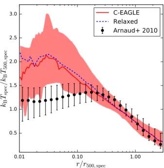
Figure 12. Median spectroscopic temperature profiles for theC-EAGLE sam-ple and the relaxed subset atz=0.1. Marker styles are identical to Fig.11. The median observed profile is calculated by combining the pressure profiles from Arnaud et al. (2010) with the entropy profiles from Pratt et al. (2010), with the error bars enclosing 1σof the sample.
gas rich. The excess gas is at radii>0.5r500,specwhere theC-EAGLE clusters have a density that exceeds the observed density profile. These results suggest that the AGN feedback in theEAGLEmodel is capable of ejecting gas from the core of the cluster, but is not moving sufficient amounts beyondr500.
We plot the median dimensionless spectroscopic temperature pro-file atz= 0.1 for theC-EAGLE clusters and the relaxed subset in Fig.12. Again, we find negligible difference between the full sam-ple and the relaxed samsam-ple. At radii greater than 0.2r500,spec, we find good agreement between the observed median profile and the C-EAGLEclusters, with both profiles showing a similar level of scat-ter. However, inside this radius the two profiles diverge significantly from each other. The observed clusters turn over at 0.2r500,spec, with a roughly flat profile in the cluster core. On the other hand, the C-EAGLEclusters have a median profile that continues to rise until 0.03r500,specand reaching a peak value≈60 per cent higher than the observed median profile. The temperature profile is consistent with the density profile, AGN feedback is ejecting and heating central gas in the cluster cores and producing a temperature profile that rises all the way to the centre of the cluster.
Figure 13. Median pressure profiles for theC-EAGLEsample and the relaxed subset atz=0.1. Marker styles are identical to Fig.11. Data points show the median observed profile from Arnaud et al. (2010), with the error bars enclosing 1σof the sample.
Figure 14. Median entropy profiles for theC-EAGLEsample and its relaxed subset atz=0.1. Marker styles are identical to Fig.11. Data points show the median observed profile from Pratt et al. (2010), with the error bars enclosing 1σ of the sample. Additionally, we show the prediction from non-radiative simulations (Voit et al.2005).
We plot the medianz=0.1 entropy profiles of theC-EAGLE clus-ters and the relaxed subset in Fig.14. Beyond a radius of 0.5r500,spec, theC-EAGLEclusters tend to the power-law result predicted by non-radiative simulations (Voit, Kay & Bryan2005). However, inside this radius the entropy profile develops a large core. The radial extent of the core region is significantly greater than observed pro-file and central value of the entropy is up to a factor of 5 larger. Observational results have shown that the central cooling times of clusters take a range of values between those that are significantly
Figure 15. Median emission-weighted iron abundance profiles for the C-EAGLEsample and its relaxed subset atz=0.1. Marker styles are identical to Fig.11. The black squares and triangles are the mean observed profiles from Leccardi & Molendi (2008) and Matsushita (2011), with the error bars showing the measurement uncertainty.
shorter than the Hubble time, ‘cool-core’ clusters with power-law-like entropy profiles, and those that are longer than the Hubble time, ‘non-cool-core’ clusters with cored entropy profiles (e.g. White, Jones & Forman1997; Peres et al.1998; Sanderson, O’Sullivan & Ponman2009; Cavagnolo et al.2009). Previous simulation work has reproduced this range of cooling times (Rasia et al.2015; Hahn et al.2017). All of theC-EAGLEclusters are non-cool-core clusters with cored entropy profiles. In agreement with the temperature pro-files, the entropy profiles suggests that the AGN feedback is heating the core of the cluster. Several of the clusters have inverted central entropy profiles, which can only be produced by a recent injection of energy as it is thermodynamically unstable. This inject of energy by the AGN quickly destroys any cool-core that begins to form.
Finally, we examine the distribution of metals throughout the cluster volume. In Fig.15, we plot the median emission-weighted iron abundance profiles atz=0.1 for theC-EAGLEclusters and the relaxed subset. We compare with the observations of Leccardi & Molendi (2008) who studied 48 clusters atz<0.3 and Matsushita (2011) who studied 28 clusters atz<0.08. We have scaled all results to the solar abundances of Asplund et al. (2009). For consistency with the observed profiles, we follow Arnaud, Pointecouteau & Pratt (2005) and calculater180,specvia
r180,spec=1.78
kBT X,ce 500,spec 5 keV
0.5
E−1
(z), (9)
wherekBT500X,ce,specis the core-excised spectroscopic X-ray tempera-ture measured by a single temperatempera-ture fit to the combined spectrum of all particles that fall within (0.15–1.0)r500,spec.
1102
D. J. Barnes et al.
that is systematically higher by 0.1 dex; however, the difference is within the intrinsic scatter of the simulated profiles.
5 D I S C U S S I O N
We have presented the global properties of theC-EAGLEclusters, a set of zoom simulations of 30 objects run with theEAGLEgalaxy formation model that yields realistic galaxies and resolves the ICM on kiloparsec scales. We did not recalibrate the model on cluster scales; instead we chose to retainEAGLE’s good match to the observed galaxy stellar mass function, the galaxy size–mass relation and the BH mass–stellar mass relation, thus extending theEAGLEresults to higher mass haloes. We found a reasonable match to observations for the total stellar content of the clusters and BH mass–stellar mass relation. The ICM properties, a prediction of a calibrated galaxy for-mation model, are a reasonable match to the properties of observed low-redshift clusters. The main exceptions are the gas fractions and the cluster entropy profiles. Both of these results suggest that the AGN feedback needs revision if it is to reproduce more realistic cluster properties.
The normalization of the gas fraction–total mass relation is high compared to the observed relation (see Figs 5 and 6). Previous work by McCarthy et al. (2011) has shown that the majority of gas expulsion from galaxy groups and clusters occurs between z
≈ 2 and 4. In our model, the first AGN feedback events occur when the BH enters its rapid growth phase, which occurs when the host halo becomes massive enough that its halo gas is too hot for supernova feedback to regulate the inflow (Bower et al.2017). Since the progenitors of higher mass haloes collapse at an earlier epoch than those of smaller haloes, they cross the mass threshold for rapid BH growth earlier when the density of the Universe is higher. This means that their potential wells are deeper, requiring more energetic feedback to expel the same fraction of gas. The higher-than-observed gas fractions of theC-EAGLEclusters suggest that AGN feedback does not inject sufficient energy into cluster progenitors at high redshift. This may also explain why the BCGs are too massive (Bah´e et al.2017), since more efficient feedback at higher redshift will also suppress star formation in cluster progenitors.
In addition, a comparison of the simulated and observed entropy profiles (Fig.14) shows that the simulated clusters have significantly larger cores, higher central entropies than observed and none of them are cool cores. This suggests that AGN feedback continues injecting energy into the cluster cores once they have formed, maintaining or increasing their size and preventing cool cores from ever reforming. AGN feedback inEAGLEuses a modified Booth & Schaye (2009) model, which is based on Springel et al. (2005). These two models have been used by several previous studies (Planelles et al.2014; Pike et al.2014; Le Brun et al.2014; McCarthy et al.2017) that broadly reproduce the observed entropy profiles of clusters. The principal difference between this study and previous work is that we achieve a mass resolution that is a factor of 100–500 times better. This lowers the energy threshold for an AGN feedback event by the same factor in our implementation. The decrease in energy threshold results in individual events that are less energetic but occur more frequently, thus rendering the feedback smoother and less episodic. In addition, the high resolution of theC-EAGLEsimulations means that the gas reaches higher densities around the central BH compared to previous studies. In a Bondi–Hoyle model, the rate of accretion scales as the mass of the BH squared. Therefore, once the cluster core has formed and the central BH is massive, even modest larger scale densities will be enhanced in the immediate vicinity of the BH and so lead to significant accretion. Thus, it is not necessary for a
cool core to reform in order to trigger an AGN feedback event, as is the case at lower resolution.
If the AGN feedback events were more energetic, they might ex-pel gas more effectively from high-redshift progenitors, potentially making gas infall and star formation less efficient. Increasing the energy threshold for individual events would also make feedback more intermittent, perhaps allowing cool cores to reform during periods of low activity. However, in the currentEAGLEmodel we are limited by the pressure–entropy SPH formalism, which fails to con-serve energy if too many particles are heated in a single time step. In addition, there are other effects to consider. The AGN feedback model currently distributes heat isotropically to the surrounding gas. If the heating was concentrated into a jet, it might allow a cool core to coexist with the transport of energy to larger radii as is observed, for example, in the Perseus cluster (e.g. Zhuravleva et al.2014). The role of our artificial conduction scheme in shaping the cluster core is also unclear. Improvement of theEAGLEAGN feedback model is ongoing, but this work highlights that we must continue to improve the modelling of processes that occur below the resolution limit of the simulations as we push to higher resolution.
6 S U M M A RY
In this paper, we have introduced the Cluster EAGLE (C-EAGLE) simulation project, a set of zoom simulations of the formation of 30 galaxy clusters in the mass range of 1014<M
200/M<1015.4that resolve the cluster galaxies and the ICM on kiloparsec scales using the state-of-the-artEAGLEAGNdT9 model ofS15. In this paper, we have presented the global cluster properties, a prediction of a model calibrated for the formation of field galaxies. The properties of the cluster galaxies are analysed in Bah´e et al. (2017). Our main results are as follows:
(i) TheC-EAGLEclusters provide a consistent extension to periodic volumes of the originalEAGLEproject, sampling the massive objects that were missing due to their limited volumes.
(ii) Estimating masses from mock X-ray observations rather than using the true mass results in a hydrostatic bias of 15–20 per cent (Fig.2). Selecting relaxed clusters produces a similar bias but sig-nificantly reduces the scatter.
(iii) The clusters show reasonable agreement with the observed relations that were used to calibrate theEAGLEmodel at lower masses. The clusters show a flat stellar fraction–total mass relation in agree-ment with the observations (Fig.3), and the trend, normalization and scatter of the BH mass–stellar mass relation are also in agree-ment with the observations (Fig.4). TheC-EAGLEclusters contain a population of orphan supermassive BHs, likely the remnants of galaxy mergers. Several of these orphans reside inside the BCGs.
(iv) TheC-EAGLEclusters reproduce the observed gas fraction– total mass trend, but the normalization is too high by≈30 per cent (Fig.5). Although we selected the AGNdT9 calibration as it better reproduced the gas fractions of low-mass galaxy groups, the dif-ferentEAGLE AGN calibrations produce similar results on cluster scales. The progenitors of clusters will form at an earlier epoch than those of less massive haloes, causing them to have deeper poten-tials due to the increased density of the Universe. The increased gas fractions suggests that in this regime theEAGLEAGN feedback model does not inject sufficient energy into the progenitors of the C-EAGLEclusters.