Minimum-Energy Broadcasting in Multi-hop
Wireless Networks Using a Single Broadcast Tree
Ioannis Papadimitriou and Leonidas Georgiadis
Abstract
In this paper we address the minimum-energy broadcast problem in multi-hop wireless networks, so that all broadcast requests initiated by different source nodes take place on thesamebroadcast tree. Our approach differs from the most commonly used one where the determination of the broadcast tree depends on the source node, thus resulting in different tree construction processes for different source nodes. Using a single broadcast tree simplifies considerably the tree maintenance problem and allows scaling to larger networks. We first show that, using the same broadcast tree, the total power consumed for broadcasting from a given source node is at most twice the total power consumed for broadcasting from any other source node. We next develop a polynomial-time approximation algorithm for the construction of a single broadcast tree. The performance analysis of the algorithm indicates that the total power consumed for broadcasting from any source node is within2H(n−1)from the optimal, wherenis the number of nodes in the network and H(n)is the harmonic function. This approximation ratio is close to the best achievable bound in polynomial time. We also provide a useful relation between the minimum-energy broadcast problem and the minimum spanning tree, which shows that a minimum spanning tree may be a good candidate in sparsely connected networks. The performance of our algorithm is also evaluated numerically with simulations.
Index Terms
Wireless Networks, Minimum-Energy Broadcast, Spanning Trees, Approximation Algorithms, Performance Analysis
I. INTRODUCTION
The field of infrastructureless wireless multi-hop networks has attracted significant attention by many researchers in the recent years because of its large number of new and exciting applications. However, the technical challenges that arise pose many new problems and issues that have to be addressed when designing a network in this field [1], [2]. Such an issue is the efficient management of the available energy resources.
A preliminary version of this work appeared in theProceedings of WiOpt’04: Modeling and Optimization in Mobile, Ad Hoc and Wireless Networks, University of Cambridge, UK, March 2004.
I. Papadimitriou and L. Georgiadis are with Electrical and Computer Engineering Department, Aristotle University of Thessaloniki, GREECE. E-mails: [email protected] , [email protected] .
One important distinction as to how energy consumption must be taken into account is whether energy is viewed as an expensive (but renewable) commodity or as a finite (and nonrenewable) resource [3].
In this paper we focus on the problem of energy-efficient broadcasting in wireless networks where omni-directional antennas are used and there is flexibility of power adjustment. As indicated in one of the pioneer
works by Wieselthieret al. in [4], broadcasting in a wireless environment where omnidirectional antennas
are used, must take into account the fact that a node’s transmission can reach multiple neighbors at the same
time. Hence, the power needed to reach a node’s set of neighbors is the maximumof the powers needed to
reach each of the neighbors separately. Given a specific source node that initiates a broadcast request, the problem of determining a set of retransmitting nodes and their corresponding transmission powers, such that
the sum of consumed node powers is minimized, is known as theminimum-energy broadcastproblem.
Although the problem of minimum-energy broadcasting has been studied extensively in the literature (see Section II for references to prior work), most of previous approaches provide a solution for it which depends on the source node that initiates the broadcast request. That is, every time a node needs to broadcast some information to all other nodes in the network, the algorithm for the broadcast tree construction is executed for the specific source node. In general, for different source nodes, the trees that minimize the total power consumption are different (see Section III-B for an example). Hence, in general, each node in the network
has to keep track of nbroadcast trees, one for each of the possible source nodes (nis the number of nodes
in the network). This requires large memory space and/or processing capabilities on behalf of the nodes in the network, a demand that cannot always be met.
The above situation will be greatly simplified if one can define asinglebroadcast tree, on which
broad-casting initiated byanysource node will take place in a predetermined manner. Hence, in our setup we are
interested in selecting a unique broadcast tree that keeps the total power consumption as small as possible for any broadcast request. In this manner, a node needs to store only a small set of links that belong in the selected tree and the processing of broadcast information is minimal. More specifically, whenever a node receives a broadcast message for the first time in one of its tree links, it forwards it with appropriate power
to all its neighbors in the tree except the one from which the message was received. Note that this is exactly how a Connected Dominating Set (CDS) would work in case we did not have the flexibility of power adjust-ment (see for example [5], [6], [7]). In this case, a single CDS is determined for the network and each node needs only to know whether it belongs to this set or not.
When nodes initiate broadcast requests at the same time, it may seem that the use of a single tree results in more collisions compared to the approach of using different trees for different source nodes. However, this is not necessarily the case. Indeed, the use of omnidirectional antennas implies that independently of the approach used (single or multiple broadcast trees) a node’s transmission will interfere with its neighbors’ transmissions or receptions. Hence, whether the node retransmission is always intended to particular desti-nations (in case of single broadcast tree) or to different destidesti-nations (according to the source node in case of multiple broadcast trees), all nodes in the neighborhood will be affected and the lower level issue of colli-sion resolution does not create a bias towards one of the methodologies. Network instances and particular broadcast scenarios can be created where one approach is better or worse than the other.
There are two open issues with our approach that have to be answered. First, if all broadcast requests take place on the same tree, then this may result in widely varying total powers for different source nodes. Second, even if a tree is found without having the drawback of resulting in widely varying total powers for different source nodes, then, for a specific source node the resulting total power consumption may be far away from the optimal. We address both issues in Section III-B and provide satisfactory answers to them in Section IV. More precisely, we first show that if the same tree is used for broadcasting by all nodes, then the total power consumed for broadcasting from a given source node is at most twice the total power consumed for broadcasting from any other source node. Next, we develop a polynomial-time approximation algorithm for the construction of a single broadcast tree. The performance analysis of the algorithm indicates that the
total power consumed for broadcasting initiated by any source node is at most2H(n−1)times the optimal
(H(n)is the harmonic function), which is close to the best achievable approximation factor in polynomial
for every possible source node. Moreover, it is valid for general networks, with arbitrary weights on links between nodes, which do not rely on unit disk graphs and geometric properties of the Euclidean space. This is a more realistic model since, for example, the power needed for communication between two pairs of nodes with equal distances between the nodes of each pair, may not be the same due to noise or other signal
propagation phenomena. We also show that the performance of theminimum spanning tree[8] is within∆
times the optimal, where∆is the maximum node degree in the network. Hence, a minimum spanning tree
can also be used for broadcasting by all nodes in sparse networks.
Numerical results for various networks with different sizes are presented in Section V. The main perfor-mance metric of interest is the total broadcast power consumption for different source nodes. It is shown that our algorithm provides fairly satisfactory performance for networks represented by unit disk graphs. However, we note that our algorithm outperforms significantly other algorithms for some interesting in-stances of general networks and, therefore, it presents a good compromise between simplicity and achieved performance.
The rest of the paper is organized as follows. In Section II we give some references to prior work related to the minimum-energy broadcast problem. Section III provides formal definitions and formulation of the problem. In Section IV we develop a polynomial-time approximation algorithm and prove that it achieves a satisfactory approximation ratio regarding the metric of total power consumption. We also provide a useful for sparse networks relation between the minimum-energy broadcast problem and the minimum spanning tree. Numerical results are presented in Section V. Finally, Section VI summarizes the conclusions of our work and presents some interesting issues for further study. All proofs of the lemmas provided in the paper are given in the Appendix.
II. RELATEDWORK
The minimum-energy broadcast problem in wireless networks has received significant attention over the
last few years. The work by Wieselthieret al. [4] exploits the “node-based” nature of wireless
of the work in [4] is the Broadcast Incremental Power (BIP) algorithm. BIP constructs a broadcast tree starting from the source node and adding to the tree one node at every iteration. The selection of which
uncovered node will be added to the tree is based on theminimum additional costcriterion. Numerical
re-sults demonstrate the advantages of BIP over conventional link-based schemes, but a performance analysis of the algorithm is not provided. In [9] the general combinatorial optimization problem, called Minimum Energy Consumption Broadcast Subgraph (MECBS), is considered. It is proved that MECBS is not ap-proximable within a sub-logarithmic factor (unless NP has slightly superpolynomial time algorithms) and a polynomial-time approximation algorithm is provided for special cases in the Euclidean space.
The NP-completeness of the minimum-energy broadcast problem is also proved in [10], [11], [12], [13]. In [10], [11], [13] various heuristic algorithms are proposed and their performance is compared numerically to that of BIP. Analytical performance results are not presented. The approximation algorithm developed in [12] and the analytical results that are provided depend on the number of adjustable power levels at each node. By exploring geometric structures of Euclidean MSTs, analytical results are also provided in [14] for BIP and other algorithms. Three different integer programming (IP) models that can be solved by any standard IP technique are proposed in [15] for the minimum-energy broadcast problem. The problem of minimum-energy broadcasting is also addressed in [16], a survey where an overview is presented of the recent progress in applying computational geometry techniques to solve some questions in wireless networks.
The first logarithmic approximation algorithm for the MECBS problem is presented in [17], where an interesting reduction to the Node-Weighted Connected Dominating Set problem is used. The proposed
algorithm achieves a 10.8 lnn approximation ratio for symmetric instances of MECBS, which is worse
than ours. Moreover, the approach followed in [17] depends on the specific source node. An improved approximation ratio, which is closer to ours (but still, slightly worse), has been independently announced
recently in [18]. The proposed algorithm improves the approximation ratio from 10.8 lnnof [17] to 2 +
on the source node; on the other hand, the algorithm in [18] is applicable to networks with asymmetric power requirements.
The problem of constructing energy-efficient broadcast and multicast trees in an energy-, bandwidth-, and transceiver-limited wireless network is addressed in [19]. Similarities and differences between energy-limited and energy-efficient communications are described and the impact of these overlapping (and some-times conflicting) considerations on network operation is illustrated. An approach to the problem of energy-aware broadcasting with emphasis on individual node power consumption is proposed in [20]. The lexico-graphic optimization criterion is introduced and the objective is to minimize lexicolexico-graphically the consumed node powers or maximize lexicographically the residual node energies. We leave the issue of addressing our model in an energy-, and resource-limited environment as a subject for further study.
III. DEFINITIONS AND PROBLEMDESCRIPTION
Consider a connected undirected graph G = (N, L), where N is the set of nodes and L is the set of
undirected links. For a nodei∈N we denote byLG(i)the set of links adjacent toi. A nodejsuch that link (i, j)belongs toLis called a one-hop neighbor ofior simply a neighbor ofi. We denote byNG(i)the set
of neighbors of nodei. An undirected treeT = (N, LT)spanningG(spanning tree for short) is a connected
acyclic subgraph that spans all the nodes. It follows from the definition of spanning tree that the number of links inT is|LT
|=|N|−1.
A. Model for Wireless Broadcasting
We model the wireless network as a connected undirected graph G = (N, L). N is the set of nodes in
the network. If nodej can successfully receive information transmitted by nodei, and vice versa, then link
(i, j)belongs to the setLof links inG. The power needed for a successful transmission over linkl = (i, j) is denoted bycl >0and is also referred to as the link cost. Each node is equipped with an omnidirectional antenna. Hence:
Note that in addition to the above power requirement, energy is also expended for transmission (encoding, modulation, etc.) and reception (demodulation,decoding, etc.) processing operations as indicated in [19]. For the analysis in the next sections, we assume that the energy consumption quantities for transmission and reception processing operations are small and thus can be neglected, an approach followed by many previous works referenced in Section II. However, we note that the incorporation of the aforementioned quantities into our model is not a major concern if the network nodes consume similar power for transmission (as well as reception) processing. More specifically, the fact that all nodes in the network (except the source node) receive the information in a broadcast process, results in adding a fixed quantity in the overall energy consumption. This does not affect the minimum-energy broadcast problem, since the total energy consumed for reception is always the same. Regarding the energy requirement for transmission processing operations, this quantity can be incorporated into the cost of each link without affecting our approach in the following sections.
Suppose that a source nodes needs to broadcast some information to all other network nodes. In this
case, we have to determine a set of retransmitting nodes and their corresponding transmission powers, so that eventually all nodes receive the information. A way to achieve this, which will be useful in the sequel,
is as follows. Let T be a spanning tree ofG. We define an s-rooted directed spanning treeTs = (N, LTs)
induced byT, with the following interpretation:
1) Node s uses all links in LT(s)as its outgoing links. We define LTs
out(s) = LT(s)and node s transmits with power pTs
s = maxl∈LTsout(s){cl}. Note that there is no link incoming to nodes in the setL
Ts, that is,
LTs
in(s) =∅.
2) Any node i of T receiving the information in one of its tree links in LT(i), say link l, uses the set
LT(i)
−{l}as its outgoing links. Therefore, we define LTs
in(i) = {l},L
Ts
out(i) = LT(i)−{l}, and nodei retransmits with powerpTs
i = maxl∈LTsout(i){cl}. We refer top
Ts
i as the power induced on nodeiby treeTs. If
LTs
out(i) =∅, theniis called aleaf node ofTsandpTis = 0.
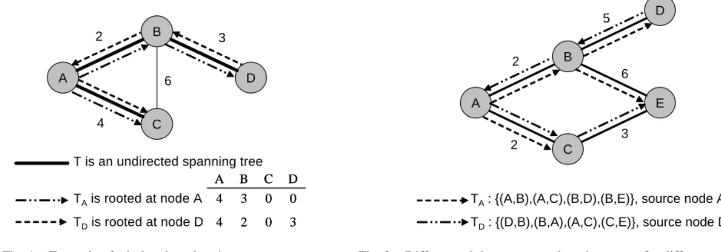
A B C D 2 4 3
TAis rooted at node A TDis rooted at node D
6 3 0 2 4 0 0 3 4 D C B A 3 0 2 4 0 0 3 4 D C B A
T is an undirected spanning tree
Fig. 1. Example of wireless broadcasting
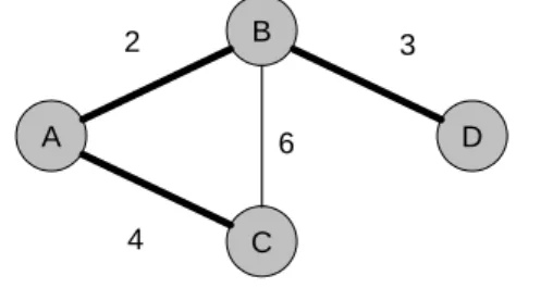
A B C D E 2 2 5 6 3
TA: {(A,B),(A,C),(B,D),(B,E)}, source node A
TD: {(D,B),(B,A),(A,C),(C,E)}, source node D
Fig. 2. Different minimum-energy broadcast trees for different source nodes
A and D respectively, are induced by the (undirected) spanning tree T with links {(A,B),(A,C),(B,D)}.
Consider for example the tree TA. The outgoing links of source node A in this case are {(A,B),(A,C)}
and the outgoing link of node B is (B,D). Hence, the powers induced on nodes A and B by treeTA are
pTA
A = 4 andp
TA
B = 3, respectively. Note that nodesC andDhave no outgoing links inTA and, therefore,
pTA
C =p
TA
D = 0. In a similar way, we have for treeTDthatpTAD = 4,p
TD
B = 2,p
TD
C = 0, andp
TD
D = 3.
B. The Minimum-Energy Broadcast Problem
Given ans-rooted directed spanning treeTs, the total power consumed for broadcasting from source node
sisP(Ts) =
P
i∈Np
Ts
i . As discussed earlier, in general, for different source nodes the trees that minimize
the sum of consumed node powers are different. Hence, each network node has to keep track of|N|broadcast
trees, one for every possible source node.
Consider for example the network in Fig. 2. The optimal (minimum-energy) broadcast trees for source
nodesAandDare the treesTAandTD, respectively. The total power consumption for these trees is
P(TA) =pTAA +pTBA = 2 + 6 = 8 and P(TD) =pTDD +pTBD +pATD +pTCD = 5 + 2 + 2 + 3 = 12.
Note that the underlying (undirected) spanning trees ofTAandTD are different. If, for example, the source
nodeDuses the underlying tree ofTAfor broadcasting, then the sum of consumed node powers will be13,
larger than the optimal value12obtained from treeTD.
The situation will be greatly simplified if one can define a single spanning treeT, on which broadcasting
a nodeineeds to store only the setLT(i)and processing of broadcast information is minimal. Hence, in our setup we are interested in selecting a unique spanning tree that keeps the total power consumption as small as possible for any source node.
There are two open issues with our approach that have to be answered; if all broadcasts (initiated by any source node) take place on the same tree, then:
Issue1:Certain broadcasts may need much more total power than others, depending on the source node.
Issue 2: If one attempts to find a tree for which the total powers consumed for broadcasting initiated by different source nodes are approximately the same, then, given a certain source node, the resulting total power may be far away from the optimal.
In the section that follows we will first show that the first concern (widely varying total powers) is not a
major problem. More precisely, we will prove that, given a spanning treeT, the total power consumed for
broadcasting based onT from a source nodes is at most twice the total power consumed for broadcasting
from any other source node. Next, we will propose an algorithm for the construction of a spanning treeT,
which has the desirable property that the resulting total power consumption for any source node is close to the computationally feasible factor from the optimal.
For the development and analysis of the algorithm presented below, we need the following general defini-tion of tree cost. This is a purely technical definidefini-tion and it has no physical interpretadefini-tion.
Definition 1: LetT be a spanning tree of G. We define Ato be a link assignment to nodes inG, which associates with each nodeia set of linksA(i)⊆ LT(i), such that
A(i)∩A(j) = ∅, wheneveri 6= j, and
∪i∈NA(i) = LT. Under link assignmentA, we define the “power” of nodei ∈ N aspAi = maxl∈A(i){cl}
and the cost of treeT asPA(T) =Pi∈N pAi .
Note that the broadcasting initiated by a given source nodesusing treeT corresponds to a particular link
assignmentAs, such thatAs(s) = LT(s)and for each nodei ∈N,i=6 s,As(i) =LT(i)−{l}, wherelis
the link ofT over which the broadcast information arrives at nodei. That is, thes-rooted directed spanning
A
B
C
D 2
4
3
y AA(A)={(A,B),(A,C)}, AA(B)={(B,D)}, AA(C)=AA(D)=Ø
y AD(A)={(A,C)}, AD(B)={(B,A)}, AD(C)=Ø, AD(D)={(D,B)}
y A(A)= Ø, A(B)={(B,A),(B,D)}, A(C)={(C,A)}, A(D)=Ø
6
T is an undirected spanning tree
Fig. 3. Various link assignments for a given spanning treeT
Hence, we have thatP(Ts) =PAs(T).
Fig. 3 shows an example of various link assignments for a given spanning treeT. Link assignmentsAA
and AD correspond to broadcasting from source nodes A andD, respectively, using tree T. Therefore, it
holdsPAA(T) =P(T
A) = 7andPAD(T) =P(TD) = 9. In contrast to link assignmentsAAandAD,Ais an example of link assignment which does not correspond to any broadcasting process. However, according to Definition 1, the cost of treeT under assignmentAis defined asPA(T) =pA
B+pAC = 3 + 4 = 7.
IV. BROADCASTING USING A SINGLEBROADCASTTREE
A. Addressing Issue 1
In order to show that using the same tree for all broadcasts does not result in widely varying total powers for different source nodes, we first provide a useful lemma. The lemma that follows indicates that, given
a spanning tree T, the cost of T under a link assignment that corresponds to broadcasting from a certain
source node is at most twice the cost ofT under any other link assignment.
Lemma 1: LetT be a spanning tree of G. If As is a link assignment that corresponds to broadcasting
from a given source nodesusing treeT andAis any other link assignment, thenPAs(T)≤2PA(T).
Consider now a source nodes0 6= s. Since the cost ofT under assignmentA
s,PAs(T), is at most twice
the cost of T under any other link assignment, it follows that PAs(T) is also at most twice the cost of T
under assignmentAs0, which corresponds to broadcasting from source nodes0using treeT. Hence, we have
the following corollary:
Corollary 1: If the same spanning tree T is used for broadcasting by all nodes, then the total power
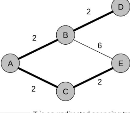
yA(A)=Ø, A(B)={(B,A),(B,D)}, A(C)={(C,A),(C,E)}, A(D)=A(E)=Ø
yAE(A)={(A,B)}, AE(B)={(B,D)}, AE(C)={(C,A)}, AE(D)=Ø, AE(E)={(E,C)}
T is an undirected spanning tree
P (T) = 4
P (T) = 8 = 2 AE yP (T)
A A
B
C
D
E 2
2
2
6
2
A
Fig. 4. A tight example for the result proven in Lemma1
from any other source node. That is, for any two nodess,s0,P(Ts) =PAs(T)≤2PAs0(T) = 2P(Ts0). Note that Lemma 1 is stronger than Corollary 1; it states that the right part of the inequality may concern
anylink assignment, not only assignments that correspond to broadcasting from a given source node.
A tight example for the result proven in Lemma 1 is provided in Fig. 4. Link assignmentAE corresponds
to broadcasting from source nodeE using treeT, whileAis a link assignment which does not correspond
to any broadcasting process. For these two assignments, it holds
PA(T) =pAB+pCA = 2 + 2 = 4 and PAE(T) =pAE
E +pA
E
C +pA
E
A +pA
E
B = 2 + 2 + 2 + 2 = 8.
Therefore,PAE(T) = 2PA(T)and this example shows that the upper bound in Lemma 1 is a tight one. A
similar example can also be constructed in case where the link assignmentA corresponds to broadcasting
from a particular source node. Consider three nodesA,B,C in tandem with link costsc(A,B) =c(B,C) = 1.
Broadcasting from source nodeAneeds power2(AtoB andBtoC), while broadcasting from source node
B directly to nodesAandCneeds power1.
B. Addressing Issue 2
We now address the second issue, that is, the problem of selecting a tree such that the resulting total power consumed for broadcasting is not far away from the optimal for any source node. A problem closely related to the one of interest (see below for an explanation of this relation) is the following:
Problem 1: Find a spanning treeT∗ and a link assignmentA∗ such that, for any spanning treeT of G
Note that if we use the treeT∗ for broadcasting from source nodes, we have according to Lemma 1 and inequality (1) that
P(Ts∗) =PA∗s(T∗)≤2PA∗(T∗)≤2PA(T). (2)
Consider now an optimal (minimum-energy) s-rooted directed spanning tree. As mentioned earlier (right
after Definition 1), this tree can be defined by an undirected spanning tree and a particular link assignment.
Since the total power consumed for broadcasting from source nodesusing treeT∗,P(T∗
s), is at most twice
the cost of T under assignment A (as indicated in (2)), where T is any spanning tree andA is any link
assignment, it follows that P(Ts∗)is also at most twice the optimal value. Therefore, T∗ has the desirable property that the resulting total power consumption is not far away from the optimal for any source node.
Hence, we are led to the problem of determiningT∗andA∗. Unfortunately, this problem is NP-complete.
The proof is based on a modification of the argument used to prove the NP-completeness of the Minimum
Broadcast Cover (MBC) problem presented in [13] and is omitted due to lack of space1. The main idea is to
reduce the weighted version of theSet Cover(SC) problem [21] to an instance of Problem 1 and show that
the SC decision problem is satisfiable if and only if the decision problem of Problem 1 is satisfiable. The argument in the proof also shows that the reduction from SC to an instance of Problem 1 preserves approxi-mation ratios. Hence, based on the corresponding result for Set Cover [22], Problem 1 is not approximable within(1−²) log(n−1), for any0< ² < 1, unless NP⊆DTIME(nO(log logn)), where DTIME(t) is the class
of problems for which there is a deterministic algorithm running in timeO(t).
The discussion above suggests that instead of finding a tree and an assignment that solve Problem 1, we should attempt to find a good approximation. We present in Fig. 5 an approximation algorithm to construct
a single spanning treeT which, as will be shown, has the desirable property in a worst case sense. At each
iteration, the algorithm maintains a forest of trees in the network, such that each node i in G belongs to
a forest tree TF = (NTF, LTF)with link assignment AF. The node “power” and the cost of a forest tree
are defined as described in Definition 1. Initially, each node constitutes a forest tree with no links assigned
1
Algorithm 1:
Initially each nodeiinGconstitutes a forest treeTFwith link assignmentAF such thatNTF ={i},LTF =AF(i) =∅,
hence,pAi F = 0.
1. Foreach nodeiinGwhich belongs to a forest treeTF with link assignmentAF do
LetL0(i) ={(i, j)∈LG(i) :j /
∈NTF}(set of links adjacent toiand terminating outside the treeT
F).
Foreach linkl∈L0(i)do
i. LetTi(l)be the set of distinct trees (other thanTF) that can be reached by nodeiwhen powerclis used. Let
alsoBi(l)be the set of links used by nodeito reach these trees in the setTi(l)(see alsoNote1). ii.Defineai(l) = (cl−piAF)/|Ti(l)|.
end do end do
2. Among all nodesi ∈ N,L0(i) 6= ∅, identify a node and a link with minimum valueai(l), say nodeimin and link
lmin ∈ L0(imin). Letamin be that value (note that, because of step4 below, there exists at least one nodeifor which
L0(i) 6= ∅, hence,aminis well defined). That is,amin = min
i∈N:L0(i)6=∅,l∈L0(i){ai(l)}. Let alsoTFmin be the tree to
which nodeiminbelongs and defineT={TFmin}∪Timin(lmin).
3. Join nodeiminwith the trees in the setTimin(lmin)using the set of linksBimin(lmin). Hence, the trees inTare merged
to a new treeT0
F with link assignmentA0F as follows: NT 0
F = ∪T F∈TN
TF,LTF0 = ¡∪T
F∈TL
TF¢ ∪B
imin(lmin),
A0
F(imin) =AF(imin)∪Bimin(lmin).
4. Ifthere is a single forest treeT then ReturnT and its corresponding assignmentA.Else,go tostep1.
Fig. 5. Approximation algorithm for the construction of a single broadcast tree
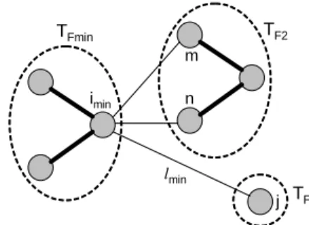
imin
j m
n
lmin
TFmin TF2
TF1
• cl
min> c(imin ,m)> c(imin ,n)andaimin(lmin) = amin
• Only one of the links (imin,m) , (imin,n) must be selected to join node iminwith the forest tree TF2 to avoid the creation of cycle
Fig. 6. Example of constructing a single broadcast tree using Algorithm1
to it. At each iteration of the algorithm, the forest is expanded by joining trees through nodes so that the “incremental power consumed per joined tree”, as defined in the algorithm, is minimal. This is achieved as
follows. For every node i in the network, we examine its adjacent links that terminate outside the tree to
which node ibelongs. For such a link l, we defineTi(l)to be the set of distinct trees that can be reached
by nodeiwhen powercl is used (a tree is “reached” by nodei, ifican reach at least one of its nodes). We
also define ai(l)to be the ratio of the “additional power” required by node ito reach the trees in Ti(l)to the number of these trees. We select a node and a link for which the quantityai(l)is minimal. Ifimin is the
selected node, then we joinimin with the appropriate trees. The set of links used for this union are assigned
Note1:When the set of linksBi(l)is determined at step1of Algorithm1, if nodeican reach a forest tree through multiple links, then only one link is chosen to avoid the creation of cycles. Consider for example the network shown in Fig. 6. Nodeiminis selected to be joined with forest treesTF1andTF2. Sinceimincan
be joined withTF2 through links(imin, m)and(imin, n), only one of these links must be chosen to avoid the
creation of cycle with links already selected at previous iterations of the algorithm. Various selection criteria (e.g., choosing a link of minimal cost) can be used. In any case, we note that the worst case performance analysis of the algorithm is not affected by the criterion used to select a link. Moreover, the simulations that we performed showed only slight differences on the total power consumption for different selection criteria.
Note 2: Algorithm1 can also be applied in the general case, where the graph G is not connected. In
this case, the algorithm constructs a spanning tree for every component of the graph, which can be used for energy-efficient broadcasting inside the component. However, the condition for the termination of the
algorithm at step4must be different. In the general case, the algorithm stops when there is no nodeihaving
at least one adjacent link that terminates outside the tree to which nodeibelongs, that is, when L0(i) = ∅
for every nodei∈N.
Our algorithm uses the notion of “minimal incremental power consumed per joined tree”. A similar notion has been used before for related problems. For example, finding the subset of “minimum weight per uncovered element” is the main idea of the well-known approximation algorithm for the weighted version of Set Cover problem [21]. A cost function similar to ours is also defined in [11], where the proposed algorithm constructs a clustering on the nodes using a function which represents the average cost induced per unmarked node. The node that (globally) has the most cost efficient range increase becomes a clusterhead and the nodes reached by the clusterhead, after its range increase, are marked. After a clustering has been found, they proceed in a second phase where they use a well-known algorithm for constructing directed minimum spanning trees [23] to join the clusters together. The algorithm in [11] computes a different broadcast tree for every possible source node and its worst case performance has not been established.
1) Performance Analysis of Algorithm 1: LetT,A be the tree and the corresponding link assignment
returned by Algorithm1. The next lemma shows that the cost ofT under assignmentAhas an approximation
ratioH(n−1)with respect to the cost of treeT∗under assignmentA∗that solve Problem 1, wheren=|N|
is the number of nodes in the network andH(n)is the harmonic functionH(n) =Pnk=1k1. Lemma 2: It holdsPA(T)≤H(n−1)PA∗
(T∗).
Combining Lemmas 1, 2, and inequality (1), it follows that if we use the treeT for broadcasting from a
given source nodes, then we have for the total power consumption that
P(Ts) =PAs(T)≤2PA(T)≤2H(n−1)PA
∗
(T∗)≤2H(n−1)PA(T), (3)
whereT is any spanning tree and Ais any link assignment ofT. Since the optimal (minimum-energy)s
-rooted directed spanning tree can be defined by an undirected spanning tree and a particular link assignment, andP(Ts)is at most2H(n−1)times the cost ofT under assignmentA(as indicated in (3)), it follows that
P(Ts)is also at most2H(n−1)times the optimal value. Hence, we have the following corollary:
Corollary 2: For any source node s, the total power consumed for broadcasting using tree T has an
approximation ratio2H(n−1)with respect to the optimal power.
2) Complexity Analysis of Algorithm 1: For the complexity analysis that follows, we assume that the
links adjacent to a nodei ∈ N are sorted in non-decreasing order of their costs. This can be made during
initialization inO(|L|log|L|) =O(|L|log|N|)time for all nodes inG.
Let us now provide the complexity for one iteration of the algorithm. For every node i ∈ N, such that
L0(i) 6= ∅, step1requires the determination of the setsT
i(l),Bi(l), and the computation of the quantities
ai(l)for eachl∈L0(i). Step2requires the identification of nodeiminand linklmin. Since the adjacent links
of a nodei∈N are sorted, we examine them in non-decreasing order of their costs. By defining appropriate
variables, we can achieve an efficient implementation for steps 1 and 2, which requires the examination
of the adjacent links of each node only once. Hence, steps 1-2 take time O(Pi∈N|LG(i)
|) = O(|L|). In step3, nodeimin is joined with the trees in the setTimin(lmin)using the set of linksBimin(lmin). Recall that T = {TFmin}∪Timin(lmin), where TFmin is the tree to which node imin belongs, and that the trees in Tare
merged to a new treeTF0. We needO(|N|) time to inform each node in the trees in Tthat it now belongs to the new treeTF0, andO(|L|)time to assign the links of the setBimin(lmin)to nodeimin. Therefore, step3
takes timeO(|N|) +O(|L|) =O(|L|).
Hence, one iteration of steps 1-4 of the algorithm requires O(|L|) time and, since at most |N|such it-erations may occur, the worst case running time of Algorithm 1 is O(|L||N|). Note that, in practice, the running time of the algorithm may be much smaller than that of the worst case, since more than two forest trees may be merged to a new tree at every iteration. Moreover, code optimization can also be made, so that only relevant links are checked in steps1-2.
C. Broadcasting using a Minimum Spanning Tree
A minimum spanning tree ofGis a spanning tree whose sum of link costs is minimal. The problem of
finding an MST has been studied extensively in the literature and polynomial-time centralized and distributed algorithms exist for its solution (see for example [8], [24]). In this subsection, we provide a simple relation between the minimum-energy broadcast problem and the minimum spanning tree, which shows that an MST can also be used for broadcasting by all nodes in sparse networks.
LetTbbe an MST, that is, a spanning tree that minimizes the costC(T) =Pl∈LT cl. Given a source node
s,Tbsis thes-rooted directed spanning tree induced byTb. Let alsoTsbe anys-rooted directed spanning tree.
The following lemma shows that if we use the tree Tbs for broadcasting from source node s, then the total
power consumption is at most ∆times the total power consumed when the treeTs is used, where∆is the
maximum node degree in the network. Lemma 3: It holdsP(Tbs)≤∆P(Ts).
Since P(Tbs) is at most ∆ times the power P(Ts), where Ts is any s-rooted directed spanning tree, it
follows thatP(Tbs)is also at most∆times the total power consumed when an optimal (minimum-energy)
s-rooted directed spanning tree is used. Hence, we have the following corollary:
Corollary 3: For any source nodes, the total power consumed for broadcasting using a minimum
We note that the proof of Lemma 3 can be used to show that the above relation between the
minimum-energy broadcast problem and the minimum spanning tree is also valid when G is a strongly connected
directed graph. In this case,∆is the maximum node outdegree in the network and the minimum spanning tree depends on the source node.
D. Issues of Distributed Implementation
Algorithm1assumes knowledge of network topology. Hence, it can be used in networks with infrequent
topological changes and low mobility [3]. In general, Algorithm1can be applied in network environments
where at least partial information of network topology is proactively maintained at each node, as in Opti-mized Link State Routing (OLSR) protocol [25]. Regarding its distributed implementation, we note that our algorithm has similarities with Kruskal’s algorithm for determining a minimum spanning tree in a connected undirected graph [8], which can also be implemented in a distributed fashion [24]. Kruskal’s algorithm builds a minimum spanning tree by adding one link at a time. At every iteration of the algorithm, a forest
of trees is maintained, as in Algorithm 1, and a link of minimal cost is selected to join two forest trees,
so that no cycle is created with previously selected links. The main difference between our algorithm and the distributed algorithm for MSTs in [24] is the manner by which the forest trees are joined, which in our case is more complicated. The issue of detailed distributed implementation and analysis of our algorithm is beyond the scope of the current work and it is a subject for further study.
V. NUMERICALRESULTS
In this section we compare numerically the performance of the following three algorithms for various networks with different sizes: 1) Broadcast Incremental Power algorithm [4] (“BIP” algorithm for short),
2) our Algorithm 1 which constructs a single broadcast tree (“SBT” algorithm), and 3) the algorithm for
determining a minimum spanning tree (“MST” algorithm). We choose BIP as the main algorithm for com-parison, because it was one of the first algorithms that exploit the node-based nature of wireless networks and it was used by many researchers to evaluate numerically the performance of other heuristic algorithms for the minimum-energy broadcast problem. We note again that BIP determines a different broadcast tree
0 1000 2000 3000 4000 5000 6000
20 40 60 80 100
Number of nodes
A v e rag e t ree p o w e r
BIP SBT MST
Fig. 7. Average tree power (over all possible source nodes) for various network sizes;a= 2, complete networks.
0 1000 2000 3000 4000
20 40 60 80 100
(T hous a n d s )
Number of nodes
A v e rag e t ree p o w e r
BIP SBT MST
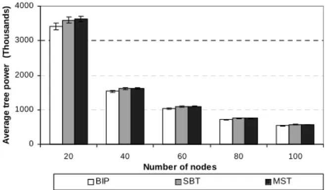
Fig. 8. Average tree power (over all possible source nodes) for various network sizes;a= 4, complete networks.
for every possible source node, while SBT algorithm constructs a single tree used by all nodes for broadcast-ing. Moreover, BIP improves its performance by using what is called the “sweep” operation, which detects redundant transmissions as well as transmissions whose power can be reduced.
The figures that follow represent the averages of the results obtained from100 randomly generated
net-work instances for each netnet-work size considered. We generate random netnet-works with a specified number of
nodes (20,40,...,100) as follows. We fix a rectangular grid of100×100 points. A number of these points
is randomly selected with uniform probability to represent the network nodes. The power needed for suc-cessful transmission over link(i, j)depends on the distanced(i,j)between the two nodes and it is given by c(i,j) =da(i,j), whereais the propagation loss exponent.
The main performance metric of interest is the total power consumed for broadcasting initiated by different source nodes. In order to quantify this metric, we introduce a closely related measure which provides the average total power consumption for broadcasting initiated by any source node. That is, for a given network
size, |N|, and for each individual network instance, we define theaverage tree power of algorithmX as
PX =
P
s∈N
P(TX
s )
|N| , whereT
X
s is thes-rooted directed spanning tree returned by algorithmX and P(TsX)is
the total power consumed for broadcasting from source node s. BIP algorithm constructs a different tree
TBIP
s for every possible source nodes∈ N, while the treesTsSBT are induced by the unique broadcast tree
returned by algorithm SBT as described in Section III-A; a single tree is also returned by algorithm MST. Fig. 7 shows the average tree power of the algorithms for various network sizes, when the propagation loss
node can successfully transmit information to all other network nodes. The symbols⊥on top of each bar represent the standard deviation of tree powers{P(TsX)}seN. We observe that SBT algorithm provides fairly satisfactory performance, comparable to that of BIP, for all network sizes considered. The average tree power of SBT is 10.9%higher than that of BIP for|N| = 20, while this percentage falls to 9.1% for|N| = 100.
The corresponding percentages for MST algorithm are16.4%and14%. The decrease in standard deviations
for all algorithms as the network size increases, is due to the fact that the trees returned by the algorithms use shorter links (links with smaller costs) as the number of nodes increases, since the density of the nodes within the same geographical area increases as well; hence, the variations in tree powers for different source nodes are smaller for larger networks. Fig. 8 provides similar results fora = 4. In this case, the average tree
power of SBT is5.2%higher than that of BIP for |N| = 20, and6.2% for|N| = 100. The corresponding
percentages for MST algorithm are 6.2% and 5.9%. We observe that the difference in performance of the
algorithms decreases as the propagation loss exponent increases. This observation conforms to results of previous works [13]. The main reason for this behavior is that the “penalty” of using longer links increases for larger values ofa. Hence, the use of such links is avoided by all algorithms and the trees returned by BIP
and SBT converge to MST whenaincreases.
The results presented thus far, show that our SBT algorithm performs fairly well for networks represented by unit disk graphs. We will now provide some interesting instances of general networks for which SBT out-performs significantly the other two algorithms. The simulations that follow attempt to model the following physical environment. Assume that the nodes are deployed on a terrain where there are various obstacles that may prohibit direct communication of certain nodes. Assume also that some of the nodes are located high up (on top of hills, buildings, etc.) so that the communication channel between these nodes and the rest of network nodes is less hostile, having smaller attenuation factor. We would like to evaluate the performance of the algorithms in such an environment.
The experiments performed in this case are the following. We set a = 2 and assume that the grid of
0.0 0.2 0.4 0.6 0.8 1.0 1.2
0.0 0.1 0.2 0.3 0.4 0.5 0.6 0.7 0.8 0.9 1.0 Factor f R a ti o r (S B T /B IP )
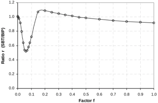
Fig. 9. Ratio of avg. tree power of SBT to that of BIP for different values of factorf;a= 2,100-node sparse networks + 1“special” node.
0.0 0.2 0.4 0.6 0.8 1.0 1.2
0.0 0.1 0.2 0.3 0.4 0.5 0.6 0.7 0.8 0.9 1.0 Factor f R a ti o r (S B T /B IP )
Fig. 10. Ratio of avg. tree power of SBT to that of BIP for different values of factorf;a= 2,100-node sparse networks + 4“special” nodes.
but, for each network instance, we include only links whose power is less thancmax, defined as the smallest
value that guarantees network connectivity. Hence, a link l between two nodes on the grid belongs to the
set L of network links if cl ≤ cmax. This constraint results in sparsely connected networks on the grid
(however, we note that the results presented below are not sensitive to the choice ofcmax; similar behavior is
observed even ifcmaxis chosen infinite, i.e., when the grid network is densely connected). After the network
on the grid is constructed, we add a “special” node in the middle of the grid and in height h = 50, that is,
the coordinates of this node are (50,50,50). We assume that the constraint on the maximum transmission
power does not hold for this additional node; hence, there is a link between this node and every other node
on the grid. The power of such a link is f ·d2, where f is a factor such that 0 < f ≤ 1, and d is the
distance in the 3-dimensional space between the “special” node and a node on the grid. An alternative
network example is to split the grid to four quarters and add4“special” nodes with coordinates(25,25,50), (25,75,50),(75,25,50),(75,75,50). Each one of these nodes is able to communicate only with nodes on the corresponding quarter of the grid.
Figures 9 and 10 present the ratior of average tree power of SBT to that of BIP for different values of
factorf, when1or4“special” nodes, respectively, are added to the100-node sparsely connected networks.
We observe that in both cases there is a range of values off for which SBT significantly outperforms BIP.
In Fig. 9, the best performance of SBT is achieved for f = 0.07(ratior = 0.225), while in Fig. 10 the
0 1000 2000 3000 4000 5000 6000
20+1 40+1 60+1 80+1 100+1 Number of nodes
A ver ag e tr ee p o w er
BIP SBT MST
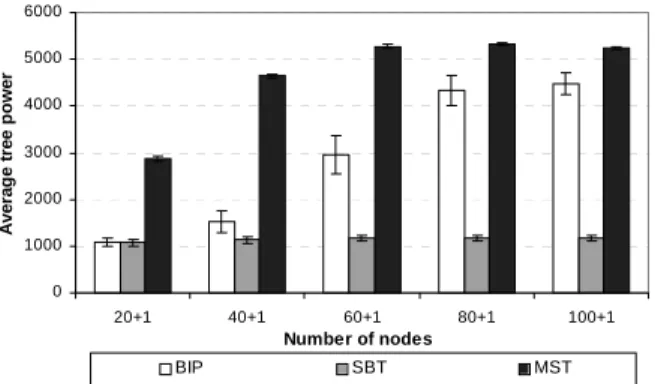
Fig. 11. Average tree power (over all possible source nodes) for various network sizes;a= 2,1“special” node added to the sparse networks, factorf= 0.1.
0 1000 2000 3000 4000 5000 6000
20+4 40+4 60+4 80+4 100+4 Number of nodes
A v e rag e tr ee p o w e r
BIP SBT MST
Fig. 12. Average tree power (over all possible source nodes) for various network sizes;a= 2,4“special” nodes added to the sparse networks, factorf= 0.1.
as follows. When f is very small (0.001 to0.02) the costs of links between the “special” nodes and nodes
on the grid are also very small, compared to the costs of links between nodes on the grid only; hence, both algorithms select the former links and construct almost identical trees (ris close to 1). The algorithms also behave almost identically (ris also close to1) when f is large (larger than0.25in Fig. 9 and0.15in Fig. 10); in this case, both algorithms avoid using links of the “special” nodes, since their costs are larger than
the costs of links between nodes on the grid. Among these two cases (very small or large values of f)
there is a range of values for which, although it is more cost efficient to use links of the “special” nodes, BIP algorithm does not succeed in selecting these links. On the other hand, SBT algorithm exploits the cost function “incremental power consumed per joined tree” and succeeds in selecting the links of “special”
nodes. Although SBT outperforms significantly BIP for a range of values offin both figures, the difference
in performance is greater in Fig. 9. This is due to the fact that in this case there is only 1“special” node
which communicates with all nodes on the grid, while in Fig. 10 there are4additional nodes and each one
of them communicates only with nodes in its corresponding quarter. Hence, the gain that SBT achieves is higher in the first case, since the cost of the constructed trees is much smaller.
The fact that SBT achieves higher gain when there is1rather than4“special” nodes can also be observed
in Figures 11 and 12, which both provide the average tree power of the algorithms for various network sizes
when the factorf is0.1. Fig. 11 corresponds to network instances with1“special” node added, while Fig.
nodes on the grid, the average tree power of BIP is 35.3% higher than that of SBT in Fig. 11, while this
percentage falls to 12.8%in Fig. 12. The corresponding percentages when there are80nodes on the grid
are270.7%and41.4%. Hence, it is concluded again, for the reason explained earlier, that the gain achieved
by SBT is higher when there is1 rather than4“special” nodes added to the network. Regarding the MST
algorithm, it performs considerably worse in both figures for all the network sizes considered.
VI. CONCLUSIONS- ISSUES FORFURTHER STUDY
In this paper we addressed the minimum-energy broadcast problem in wireless networks, so that all broad-cast requests initiated by different source nodes take place on the same broadbroad-cast tree. The main contribution is that we do not have to determine a different broadcast tree every time a source node initiates a broadcast request. Moreover, the provided results are valid for general networks and do not rely on unit disk graph models and geometric properties of the Euclidean space. We first showed that using the same broadcast tree does not result in widely varying total powers for different sources. We next developed a polynomial-time approximation algorithm to construct a single broadcast tree and analyzed its performance. We also pro-vided a useful relation between the minimum-energy broadcast problem and the minimum spanning tree, and evaluated numerically with simulations the performance of our algorithm.
There are some interesting issues for further study that arise from our work. In this paper, we consid-ered general undirected graphs to model the wireless network; however, the development of an appropriate algorithm in case of directed networks with asymmetric power requirements (different costs between two opposite directed links) remains an open problem. The distributed implementation of our algorithm could also be desirable in network environments with high mobility and frequent topological changes. Another important issue is the construction of a unique multicast tree, in case where only a subset of the nodes in the network need to communicate in an energy-efficient way. A trivial solution in this case would be to employ the broadcasting algorithm presented in this paper and then prune the resulting tree, so that only the multicast group nodes are located at the leaves of the tree. However, it might be possible to provide better solutions by looking directly at the multicast problem. In any case, we note that the adaptation of the proof of Lemma
1 for the multicast problem is straightforward and, hence, Corollary 1 also holds for the multicasting case. Finally, addressing our model in an energy-, and resource-limited environment where the maximization of network lifetime is the primary objective, is also an interesting subject which requires additional parameters, such as the initial battery energy of each node, to be considered and incorporated into the model.
REFERENCES
[1] I.F. Akyildizet al., “Wireless sensor networks: a survey,”Computer Networks, vol. 38, no. 4, March 2002, pp. 393-422.
[2] A.J. Goldsmith and S.B. Wicker, “Design challenges for energy-constrained ad hoc wireless networks,”IEEE Wirel. Commun., vol. 9, no.
4, Aug. 2002, pp. 8-27.
[3] A. Ephremides, “Ad hoc networks: not an ad hoc field anymore,”Wirel. Commun. Mob. Comput., vol. 2, no. 5, Aug. 2002, pp. 441-448.
[4] J.E. Wieselthier, G.D. Nguyen, and A. Ephremides, “Energy-efficient broadcast and multicast trees in wireless networks,”MONET, vol. 7,
no. 6, Dec. 2002, pp. 481-492. A preliminary version of this paper appearedin Proc. IEEE INFOCOM, March 2000, pp. 585-594.
[5] S. Guha and S. Khuller, “Approximation algorithms for connected dominating sets,”Algorithmica, vol. 20, no. 4, Apr. 1998, pp. 374-387.
[6] K.M. Alzoubi, P.-J. Wan, and O. Frieder, “Distributed heuristics for connected dominating sets in wireless ad hoc networks,”J. of Commun.
and Networks, vol. 4, no. 1, March 2002, pp. 22-29.
[7] J. Wu, B. Wu, and I. Stojmenovic, “Power-aware broadcasting and activity scheduling in ad hoc wireless networks using connected dominating sets,”Wirel. Commun. Mob. Comput., vol. 3, no. 4, June. 2003, pp. 425-438.
[8] R.K. Ahuja, T.L. Magnanti, and J.B. Orlin,Network Flows: Theory, Algorithms, and Applications, Prentice Hall, 1993.
[9] A.E.F. Clementiet al., “On the complexity of computing minimum energy consumption broadcast subgraphs,”in Proc. Symp. on Theor.
Aspects of Comp. Science, Feb. 2001, pp. 121-131.
[10] F. Li and I. Nikolaidis, “On minimum-energy broadcasting in all-wireless networks,”in Proc. IEEE Local Computer Networks, Nov. 2001,
pp. 193-202.
[11] A. Ahluwalia, E. Modiano, and L. Shu, “On the complexity and distributed construction of energy-efficient broadcast trees in static ad hoc wireless networks,”in Proc. Conf. on Inform. Sciences and Systems, March 2002.
[12] W. Liang, “Constructing minimum-energy broadcast trees in wireless ad hoc networks,”in Proc. ACM MOBIHOC, June 2002, pp. 112-122.
[13] M. ˇCagalj, J.-P. Hubaux, and C. Enz, “Minimum-energy broadcast in all-wireless networks: NP-completeness and distribution issues,”in
Proc. ACM MOBICOM, Sep. 2002.
[14] P.-J. Wanet al., “Minimum-energy broadcasting in static ad hoc wireless networks,”Wirel. Networks, vol. 8, no. 6, Nov. 2002, pp. 607-617.
[15] A.K. Daset al., “Minimum power broadcast trees for wireless networks: integer programming formulations,”in Proc. IEEE INFOCOM,
March-Apr. 2003.
[16] X.-Y. Li, “Algorithmic, geometric and graph issues in wireless networks,”Wirel. Commun. Mob. Comput., vol. 3, no. 2, March. 2003, pp.
119-140.
[17] I. Caragiannis, C. Kaklamanis, and P. Kanellopoulos, “A logarithmic approximation algorithm for the minimum energy consumption broadcast subgraph problem,”Inform. Proc. Letters, vol. 86, no. 3, May 2003, pp. 149-154.
[18] G. C˘alinescuet al., “Network lifetime and power assignment in ad hoc wireless networks,”in Proc. European Symp. on Algorithms, Sep.
2003, pp. 114-126.
[19] J.E. Wieselthier, G.D. Nguyen, and A. Ephremides, “Resource management in energy-limited, bandwidth-limited, transceiver-limited wireless networks for session-based multicasting,”Computer Networks, vol. 39, no. 2, June 2002, pp. 113-131.
[20] I. Papadimitriou and L. Georgiadis, “Energy-aware broadcasting in wireless networks,”in Proc. WiOpt, March 2003, pp. 267-277.
[21] V.V. Vazirani,Approximation Algorithms, Springer-Verlag, 2001.
[22] U. Feige, “A threshold oflnnfor approximating set cover,”J. of ACM, vol. 45, no. 4, July 1998, pp. 634-652.
[23] P.A. Humblet, “A distributed algorithm for minimum weight directed spanning trees,”IEEE Trans. Commun., vol. 31, no. 6, June 1983,
pp. 756-762.
[24] R.G. Gallager, P.A. Humblet, and P.M. Spira, “A distributed algorithm for minimum-weight spanning trees,”ACM Trans. on Progr. Lang.
and Systems, vol. 5, no. 1, Jan. 1983, pp. 66-77.
[25] T. Clausen and P. Jacquet, “Optimized link state routing protocol,”IETF Internet Draft, draft-ietf-manet-olsr-11.txt, July 2003 (Work in
progress).
APPENDIX
A. Proof of Lemma 1
Consider a nodei ∈ N. Note that due to Definition 1 of node “power”, if all links inAs(i)are included
in A(i), then pAs
i ≤ pAi . The latter statement and the fact that ∪i∈NA(i) = LT imply that ifpAi s > pAi , then there is at least one linkl0 in the setA
s(i)with costcl0 = pAi s, which is assigned to a neighbor node
j ∈NT(i)under link assignment
A. Sincel0 may not be the only link assigned to nodej under assignment
A, using again the definition of node “power”, we conclude that in this case it holdspAs
i =cl0 ≤pAj . Hence, in general we can writepAs
i ≤pAi +pAji, wherep
A
ji = 0for a nodeifor whichAs(i) =∅, while for a nodei
for whichAs(i) 6=∅,(i, ji)∈ As(i)andji is the neighbor ofiinT whose “power” is maximal under link assignmentAamong any other nodej such that(i, j)∈As(i). Therefore,
X
i∈N
pAs
i ≤
X
i∈N
pAi +
X
i∈N
pAji. (4)
Recall now that As corresponds to broadcasting from a given source node s using treeT. Since(i, ji) ∈
As(i)for a nodeifor whichAs(i)6=∅, the set of linksLT(ji)−{(i, ji)}is assigned to nodeji under link assignmentAs. That is, there can be no other nodei0 such that(i0, ji)∈ As(i0). Therefore, it holdsji 6=ji0 for any two nodesi 6= i0 for whichA
pAji = 0for a nodei for which As(i) = ∅, it is concluded that all terms in
P
i∈NpAji are also included in
P
i∈NpAi (zero terms do not contribute to a sum in any case). Hence,
P
i∈NpAji ≤
P
i∈NpAi and inequality (4) givesPi∈NpAs
i ≤2
P
i∈NpAi ⇒PAs(T)≤2PA(T).
B. Proof of Lemma 2
Let bk be the number of forest trees at the beginning of kth iteration. Therefore, we have b1 = n. If
the algorithm takesK iterations to complete, then we definebK+1 = 1. It follows that atkth iteration, the
number of links that join nodeiminwith the trees in the setTimin(lmin)at step3of Algorithm1isbk−bk+1
(note thatbk−bk+1 is equal to the cardinality of setTimin(lmin)). Letqk be the extra power needed by node
imin to reach thebk−bk+1 forest trees at thekthiteration. We will show that qk ≤
bk−bk+1 bk−1
PA∗(T∗). (5)
The above inequality implies the lemma. To see this, sum (5) over allK iterations to obtain
K
X
k=1
qk≤ K
X
k=1
bk−bk+1 bk−1 ·
PA∗(T∗). (6)
Note that for a certain nodei∈ N, the “power” ofiunder assignmentA(see Definition 1),pA
i , is equal to the sum over allK iterations of the powersqk that correspond to that nodei. That is,
pAi = K
X
k=1
(qk·1(powerqkcorresponds to nodei)), (7)
where the indicator function is included to denote whether each one of the powers qk, 1 ≤ k ≤ K,
cor-responds to node i. From the definition of the cost of tree T under assignment A (see Definition 1) and
equality (7), it follows that
PA(T) =X
i∈N
K
X
k=1
(qk·1(powerqkcorresponds to nodei)) = K
X
k=1
qk. (8)
Observe also that
bk−bk+1 terms bk−bk+1
bk−1 =
z }| {
1
bk−1
+ 1
bk−1
+...+ 1
bk−1 ≤ 1
bk−1
+ 1
bk−2
+...+ 1
bk+1 .
K
X
k=1
bk−bk+1 bk−1 ≤
n−1
X
k=1
1
k =H(n−1). (9)
From (6), (8), and (9), the lemma is concluded. Let us now prove (5). The treeT∗ is a spanning tree and,
hence, it spans all nodes in G. This implies that it also joins the bk forest trees at the beginning of kth
iteration with at leastbk−1links. Each of these links is assigned according toA∗ to exactly one node. Let
U be the set of nodes inT∗to which these links are assigned. For a nodei∈U, letl0be the link with largest cost among the aforementioned links that have been assigned to it. Let alsoni(l0)be the number of distinct
forest trees (other than the tree to which node ibelongs) that can be reached by iwhen power cl0 is used.
SinceT∗ joins theb
kforest trees with at leastbk−1links, it holds
X
i∈U
ni(l0)≥bk−1. (10)
By the definition of the quantitiesai(l)at thekthiteration of Algorithm1, we have min
l∈L0(i){ai(l)}≤
cl0 −pAi F
ni(l0) ≤
pA∗
i
ni(l0)
, (11)
where the second inequality in (11) is due to the fact that pAF
i ≥ 0and that the link l0 may not have the
largest cost among all links that are eventually assigned to node iaccording to A∗. From (10) and (11) it
follows that X
i∈U
pA∗ i min
l∈L0(i){ai(l)}
≥bk−1. (12)
SincePA∗(T∗)is the sum of “powers”piA∗,i∈N, andU ⊆N, it holds
PA∗(T∗)≥X
i∈U
pAi ∗ ⇒ P
A∗(T∗) amin ≥
X
i∈U
pA∗ i
amin. (13)
Sinceaminis the minimum of quantitiesai(l),i∈N such thatL0(i)6=∅,l∈L0(i), it follows from (12) and
(13) that PA∗(T∗)
amin ≥bk−1. (14)
By the definition ofaminat thekthiteration, we have
amin = qk
bk−bk+1
. (15)
C. Proof of Lemma 3
Note that for a nodeiin the treeTs, it holds max
l∈LTsout(i)
{cl}≤
X
l∈LTsout(i)
cl≤∆ max
l∈LTsout(i)
{cl}. (16)
Using the first of the above inequalities, we have
P(Tbs) =
X
i∈N
pTbs
i =
X
i∈N
max
l∈LTsoutb (i)
{cl}≤
X
i∈N
X
l∈LTsoutb (i)
cl =
X
l∈LTsb
cl =C(Tbs). (17)
SinceTbsis induced byTb, which is an MST, it follows from (17) and the second inequality in (16) that
P(Tbs)≤C(Ts) = P
l∈LTs
cl = P
i∈N
P
l∈LTsout(i)
cl ≤ P
i∈N
Ã
∆ max
l∈LTsout(i){
cl}
!
=∆P
i∈N
pTs