SEPARATION AND IDENTIFICATION TECHNIQUES FOR MEMBRANE PROTEINS USING ULTRA-HIGH PRESSURE LIQUID CHROMATOGRAPHY COUPLED TO MASS
SPECTROMETRY
Stephanie Marie Moore
A dissertation submitted to the faculty of the University of North Carolina at Chapel Hill in partial fulfillment of the requirements for the degree of Doctor of Philosophy in the Department
of Chemistry.
Chapel Hill 2016
Approved by:
James W. Jorgenson Mark H. Schoenfisch Gary L. Glish
ii © 2016
iii ABSTRACT
Stephanie Marie Moore: Separation and Identification Techniques for Membrane Proteins using Ultra-High Pressure Liquid Chromatography coupled to Mass Spectrometry
(Under the direction of James W. Jorgenson)
Due to the importance of membrane proteins in biological pathways, the development of analytical techniques to improve membrane protein identifications is essential. For such
complex mixtures, high resolution liquid chromatography (LC) is commonly utilized along with mass spectrometry (MS) for comprehensive proteomic analysis. However, commercial LC systems cannot provide the peak capacity required for such complex mixtures. With the advent of ultra-high pressure liquid chromatography (UHPLC) and multidimensional chromatography applications, peak capacities and protein identifications have increased. This dissertation will examine aspects of membrane protein sample preparation as well as instrumental analysis. Sample preparation techniques, specifically for membrane proteins, are crucial for proper protein analysis. Techniques involved with cell lysis, membrane protein extraction,
solubilization, and digestion, are discussed (Chapter 2). Ultimately an optimized membrane protein sample preparation protocol was developed involving the use of high frequency sonication and the detergent sodium deoxycholate to improve solubilization.
Peptides were ultimately analyzed on a modified (in-house) UHPLC constant pressure system. To improve proteomic separations, a new freeze/thaw valve and gradient storage loop were introduced to the UHPLC system, improving membrane protein identifications,
instrumental reproducibility, and ruggedness (Chapter 3). To improve membrane protein digestion, an immobilized enzyme reactor (IMER) was introduced to the current
iv
v
ACKNOWLEDGEMENTS
Since my decision to return to graduate school, my family has been nothing but supportive and there is no way I could have undergone this task without them. They have taught me to believe in myself and instilled a drive in me to always accomplish my goals. Being close to my family emotionally and geographically these past 5 years has been instrumental in my success, as their help and encouragement kept me focused and steadfast. This document, and my degree, would simply not have happened without them. As per our agreement, I would like to specifically thank my brother Sean for his computer expertise. It’s good to know I’m not the only Geek in the family.
I would also like to thank Chris, my partner in life, for his support and the long hours he’s put into listening to my struggles. You are my love. Of course school is nothing without the friends you make along the way and the lab mates you depend on for support. Brittany, how would we have known it was Friday without you? And Dan, no one has listened to me complain more than you, and I appreciated every time you put my concerns into perspective. I would also like to thank Kaitie Fague for introducing me to the world of proteomics and being an excellent teacher and friend.
I consider myself extremely lucky to have had the opportunities I’ve had at UNC and to learn from the best. Working with and constantly learning from my advisor, James W.
vi
vii
TABLE OF CONTENTS
LIST OF TABLES ... xii
LIST OF FIGURES... xiv
LIST OF ABBREVIATIONS AND SYMBOLS ... xxiv
CHAPTER 1: Introduction to Membrane Proteomic Analysis Using Multidimensional Liquid Chromatography – Mass Spectrometry ... 1
1.1 Introduction to Proteomics ... 1
1.2 Membrane Proteins ... 2
1.3 The Tools of Proteomics ... 3
1.3.1 Separation Techniques ... 4
1.3.2 Mass Spectrometry ... 6
1.4 Multidimensional Separations ... 10
1.5 Fully Automated On-line Proteomic Workflow ... 13
1.6 Introduction to Ultra High Pressure Liquid Chromatography ... 14
1.7 Scope of Dissertation ... 16
1.8 Figures ... 18
1.9 References... 25
CHAPTER 2: Extraction, Purification, Solubilization, and Digestion Techniques for Membrane Proteomics ... 29
viii
2.1.1 Cell Lysis Techniques ...30
2.1.2 Enrichment Techniques ... 32
2.1.3 Solubilization Techniques ... 32
2.1.4 Digestion Techniques ... 34
2.1.5 Workflow Summary... 35
2.2 Materials and Methods ... 36
2.2.1 Cell Culture and Extraction... 36
2.2.2 Enrichment ...38
2.2.3 Protein Separation and Fractionation ... 39
2.2.4 Solubilization ... 40
2.2.5 Digestion ... 41
2.2.6 Peptide Separation and Protein Identification ... 41
2.3 Results and Discussion ... 43
2.3.1 Cell Lysis... 43
2.3.2 Enrichment ... 43
2.3.3 Solubilization ... 44
2.3.4 Digestion ... 45
2.3.5 Protocol Comparison ... 47
2.4 Conclusions...48
2.5 Tables ... 50
2.6 Figures ... 56
ix
CHAPTER 3: Advances in Ultra-High Pressure Liquid Chromatography
(UHPLC) ... 70
3.1 Introduction ... 70
3.1.1 Previous UHPLC System Operation and Considerations ... 71
3.1.2 Valves and Fittings ... 73
3.1.3 Freeze/Thaw Valve ... 74
3.1.4 Gradient Storage System ... 76
3.2 Materials and Methods ... 77
3.2.1 Original UHPLC System... 77
3.2.2 Freeze/Thaw Valve ... 79
3.2.3 Gradient Storage Comparison ... 81
3.2.4 Comparison of UHPLC Systems Using a Yeast Cell Lysate ...82
3.2.5 Post Column Connection and Bleed Valve ...84
3.3 Results and Discussion ...84
3.3.1 Freeze/Thaw Valve ...84
3.3.2 Gradient Storage ... 87
3.3.3 Setup Comparison with Yeast Cell Lysate ...89
3.3.4 Post Column Connection and Bleed Valve ... 91
3.4 Conclusions... 93
3.5 Tables ... 94
3.6 Figures ... 100
x
CHAPTER 4: Characterization of an Immobilized Enzyme Reactor (IMERs) for
On-line Protein Digestion ... 127
4.1 Introduction ... 127
4.1.1 Immobilized Trypsin Digestion Strategies ... 128
4.1.2 Immobilization of Trypsin ... 129
4.1.3 Characterization of Immobilized Trypsin Particles ... 130
4.1.4 Implementation of an IMER into a Proteomic Workflow ... 132
4.2 Materials and Methods ... 133
4.2.1 Immobilization Protocols ... 133
4.2.2 Determining Trypsin Activity of Particles in a Slurry ... 134
4.2.3 Determining the Amount of Trypsin Immobilized... 135
4.2.4 Packing the Trypsin IMER ... 135
4.2.5 Determining the Activity of the IMER ... 136
4.2.6 Prefractionation Workflow ... 137
4.2.7 Analysis of Model Protein Bovine Serum Albumin (BSA) ... 139
4.2.8 Analysis of Yeast Cell Lysate ... 139
4.3 Results and Discussion ...141
4.3.1 Immobilization of Trypsin ...141
4.3.2 Immobilized Trypsin Reproducibility and Retained Activity ...141
4.3.3 Proteomics Perspective ... 142
4.3.4 IMER Characterization ... 143
4.3.5 Model Protein Results ... 144
xi
4.4 Conclusions... 146
4.5 Tables ... 148
4.6 Figures ... 155
4.7 References... 176
CHAPTER 5: Fully Automated LC-IMER-LC-MS On-line Digestion ... 180
5.1 Introduction ... 180
5.1.1 Previous 2D On-line Digestion Strategies... 182
5.1.2 IMER On-line Workflow Considerations ... 184
5.1.3 Actual Residence Time ... 185
5.1.4 Analysis of Standards and Yeast Cell Lysate... 186
5.2 Materials and Methods ... 186
5.2.1 Actual Residence Time Evaluation ... 186
5.2.2 RPLC-IMER-RPLC-MS ... 187
5.2.3 Comparison to In-solution Digestion ... 189
5.2.4 Sample Preparation Analysis ... 190
5.3 Results and Discussion ...191
5.3.1 Actual Protein Residence Time ...191
5.3.2 LC-IMER-LC-MS ... 193
5.3.3 Analysis of the Insoluble Portion of a Yeast Cell Lysate ... 194
5.4 Conclusions... 197
5.5 Tables ... 199
5.6 Figures ... 205
xii
LIST OF TABLES
Table 2.1 Default digestion protocol adapted from:
http://www.genome.duke.edu/cores/proteomics/sample-preparation51 ... 50 Table 2.2 Software Processing Parameters ... 51 Table 2.3 Overall results for extraction, enrichment, solubilization, and
digestion experiments. Experimental details held constant for
each study are outlined. ... 52 Table 2.4 Experimental design to determine the most promising
candidate for tandem digestions. ... 53 Table 2.5 Experimental results for preliminary digestions with model
proteins. ... 54 Table 2.6 Shotgun digestion protocols: Improved Protocol vs. FASP
Protocol with insoluble portion of a yeast cell lysate. ... 55 Table 3.1 nanoAcquity software program for gradients. The highlighted
rows are controlling the gradient volume. A curve of 11 is immediate; a curve of 6 is a linear change. This is specifically for the 5 μL gradient volume, however changing the time between 2.8 and 3.8 min was used to increase the gradient
volume to 10, 20, 30, and 40 μL when desired... 94
Table 3.2 Default in-solution digestion protocol adapted from:
(http://www.genome.duke.edu/cores/proteomics/sample-preparation)22... 95 Table 3.3 Software Processing Parameters ... 96 Table 3.4 Expected elution time of programed gradients for restrictor
flow rate of 300 nL/min at 30,000 psi. Restrictor was at room
temperature (25 °C). ... 97 Table 3.5 Results comparing FT valve to Pin valves using standard
protein BSA. Setups refer to those outlined in Figure 3.13 ...98 Table 3.6 Comparison of post column-pigtail connections using standard
protein BSA. ... 99 Table 4.1 Gradient method on PLRP-S column for BAEE analysis and
BSA elution. Mobile phases consisted of water (A) and
acetonitrile (B) with 0.1% trifluoroacetic acid (TFA). ... 148 Table 4.2 Various percent organic combinations tested on the IMER.
xiii
Table 4.3 Default in-solution digestion protocol adapted from: (http://www.genome.duke.edu/cores/proteomics/sample-preparation)43 Reduction and alkylation steps (d through h)
were also performed on IMER samples. ... 150 Table 4.4 Software Processing Parameters ... 151 Table 4.5 Retained Percent Activities for 8 IMERs. Manufacturer
reported trypsin activity of 10,350 BAEE units/mg trypsin. ... 152 Table 4.6 Mobile phase composition compared to actual percent organic
present. ... 153 Table 4.7 Analysis of BSA on pre-fractionation workflow with and
without IMER digestion. ... 154 Table 5.1 Gradient method on XBridgeTM column(s) for peptide
separation post-IMER. Mobile phases consisted of water (A)
and acetonitrile (B) with 0.1% formic acid (FA). ... 199 Table 5.2 Software Processing Parameters ... 200 Table 5.3 Gradient method on PLRP-S column for standard protein
analysis in the first-dimension. Mobile phase A consisted of water:acetonitrile:isopropanol (80:10:10) and mobile phase B consisted of acetonitrile: isopropanol (50:50) with 0.1%
trifluoroacetic acid (TFA). ... 201 Table 5.4 In-solution digestion protocol adapted from:
(http://www.genome.
duke.edu/cores/proteomics/sample-preparation)16 ... 202 Table 5.5 Peak parameters calculated with BA/BAEE. The values are the
average of three runs on each configuration (PLRP or
PLRP-IMER). ... 203 Table 5.6 Second-dimension peptide results for analysis of four standard
xiv
LIST OF FIGURES
Figure 1.1 Modern toolbox for proteomic analyses including sample preparation, chromatographic separation, mass spectrometry
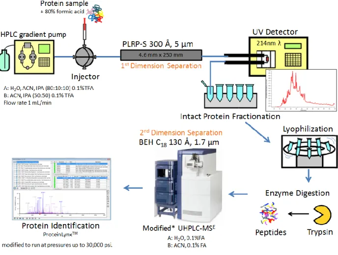
detection, and data analysis ... 18 Figure 1.2 Standard proteomic workflow for the Jorgenson lab. Proteins
are first separated on a reverse phase column followed by fraction collection and lyophilization. The proteins are digested in-solution with trypsin and the peptides are
separated on a second dimension reverse phase column with
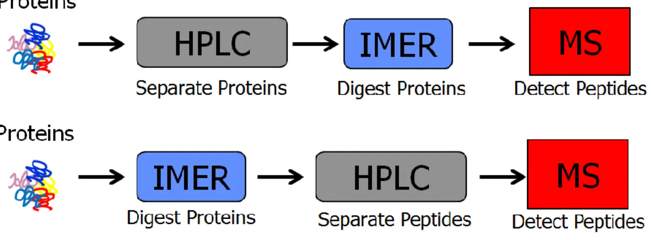
mass spectrometry detection and data analysis. ... 19 Figure 1.3 Common workflows implementing immobilized enzyme
reactors (IMERs) placed before or after the separation column. ... 20 Figure 1.4 A sample of Mass PREPTM E. coli digest standard injected on
the UHPLC system with a 50 cm x 75 μm I.D. column packed with 1.7 μm BEH C18 particles at three various pressures.
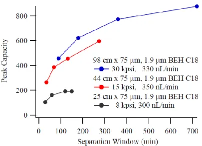
Gradient was from 5-40% acetonitrile. ... 21 Figure 1.5 Gain in peak capacity seen by implementing longer
chromatographic columns, increasing the separation space for complex sample analysis. Reproduced with permission from
the dissertation of K.Fague.41 ... 22 Figure 1.6 Original design of the ultra-high pressure liquid
chromatography system (UHPLC). ... 23 Figure 1.7 Comparison of three columns of different length analyzed with
MassPREPTM digestion standard expression mixture 2. Due to the length of these columns the pressure was increased (~30 kpsi) using the UHPLC system. For comparison (black line) a commercial column packed with the same material (1.9 μm BEH C18) was used to separate the mixture at commercial pressures (~8 kpsi). Reproduced with permission from the
dissertation of K.Fague.41 ... 24 Figure 2.1 Experimental outline. Sample preparation techniques from
four categories (cell lysis, enrichment, solubilization, and digestion) of the membrane protein workflow were compared. Each category was tested sequentially while keeping the remaining categories constant according to the default
xv
Figure 2.2 Off-line two dimensional prefractionation workflow for
membrane protein analysis. ... 57 Figure 2.3 Calculating equal mass fractions from equal time fractions.
The UV trace for the gradient elution of intact membrane protein sample (red line), where each minute represents one fraction collected (x-axis). The intensity of the UV trace is integrated and normalized to the most intense signal (y-axis). The blue line represents the summed integrated area. Since this area is proportional to concentration, the area is split into the number of desired fractions along the y-axis (for example 10 as shown here and used in this study). To determine which of the collected minute-wide fractions to combine for equal mass fractionation, the y-axis is followed over until it reaches the summed integrated area and dropped down as shown. For example, equal mass fraction seven should contain equal time fractions 32.5-35.5. Equal time fractions are not further divided to account for this, so fraction 7 becomes 32-35 or
33-36 as per the users’ discretion. ... 58 Figure 2.4 Results comparing enrichment techniques: (I) total protein
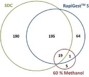
identifications and (II) membrane protein identifications. ... 59 Figure 2.5 Determining the appropriate amount of detergent. A variety of
concentrations were tested for both sodium deoxycholate (SDC) and RapiGest SF. Amount of protein used was ~30 μg
of the insoluble portion of yeast cell lysate (shotgun digestion). ... 60 Figure 2.6 Membrane protein identifications comparing 1 % SDC, 0.15%
RapiGestTM SF, and 60% methanol solubilization. ... 61 Figure 2.7 Experimental results for digestions of RNAse A with (a)
trypsin, (b) pepsin, and (c) a tandem digestion (trypsin followed by pepsin). RNAse A is plotted based on the average amino acid hydropathy score vs. peptide position within the protein. Separate red bars represent two replicates of each digestion and areas where peptides were identified are
highlighted in red. The scores are plotted from amino (left) to
carboxy (right) terminus. ... 62 Figure 2.8 Fractions collected from 1 mg of insoluble cell lysate were split
xvi
membrane protein identifications, total peptide
identifications, and membrane protein peptide identifications. ... 63 Figure 2.9 The log of the intensity ratio vs. molecular weight for the 176
membrane proteins identified using both the improved and default protocol. Proteins represented above zero (163 proteins) had a higher intensity using the improved protocol and proteins represented below zero (13 proteins) had a higher
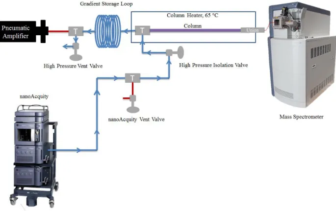
intensity using the default protocol. ... 64 Figure 3.1 Original Ultra-High Pressure Liquid Chromatography
(UHPLC) instrument design. The commercial nanoAcquity pump was used to push mobile phase and sample into the gradient storage system. Three mechanical pin vales were used to control the direction of flow within the system (high pressure vent valve, nanoAcquity vent valve, high pressure isolation valve). All plumbing consisted of 50 μm I.D. silica capillary connected to unions via proprietary capillary
connections. ... 100 Figure 3.2 Chromatographic results for Enolase standard protein digest
with: (a) no leaks present, (b) leak is present resulting in lower flow rate (longer retention times) and lower intensity peaks (less protein identifications), and (c) over time the leak worsens resulting in even lower intensities and longer
retention times. ... 101 Figure 3.3 Gradient loading profile example for the nanoAcquity pump.
The wash (i.e. high organic/B) is loaded first, followed by the gradient in reverse order (high percent B to low percent B), and finally the sample itself. The sample is sandwiched between two plugs of aqueous solvent to deter mixing prior to separation. Typical loading flow rates for the nanoAcquity are
3-5 μL/min. ... 102 Figure 3.4 Gradient and sample loading configuration for UHPLC
analysis. The commercial system loads the gradient (in
reverse) followed by the sample into the gradient storage loop. Mechanical pin valves are used to direct flow of liquid through the 50 μm I.D. external capillary plumbing. For the gradient and sample loading configuration shown here, the
nanoAcquity vent valve is closed while the high pressure vent
valve and high pressure isolation valve are open. ... 103 Figure 3.5 UHPLC high pressure run configuration. In this configuration
xvii
high pressure vent valve and the high pressure isolation valve are closed, allowing the pneumatic amplifier to engage, pushing the sample followed by the gradient onto the
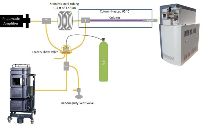
analytical column for mass spectral detection... 104 Figure 3.6 Original setup for implementation of the freeze/thaw valve. In
this configuration the mechanical pin valve would immediately halt flow to allow the FT valve to freeze a plug of liquid inside
of the capillary... 105 Figure 3.7 Original configuration of the gradient storage loop consisting
of 40 m of 127 μm I.D. stainless steel tubing. ... 106
Figure 3.8 FT valve designed from Waters Patent No. US 7,841,190 B2.11 Top and bottom are the UltemTM plastic housing (the “hive”). There is a hole in the top where the liquid CO2 enters. In the middle is the copper cup with a 10 μm sintered stainless steel filter cup placed inside (steel cup not shown in figure) The
bottom is held in place with two screws. ... 107 Figure 3.9 Schematic of the setup for the UHPLC FT Valve. The
nanoAcquityTM software activates external MOSFET switches which drive 24 V DC loads. When a high pressure run is active the temperature controller is turned on. The switch in the temperature controller turns off/on an external solenoid valve which allows liquid CO2 into the system. This freeze the liquid inside of the capillaries running through the base of the copper cup. When rapid cycling is required a second MOSFET switch allows the power from an external DC power supply to a
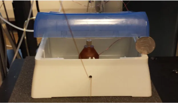
thermoelectric heater to thaw the system. ... 108 Figure 3.10 FT valve setup as implemented on the UHPLC system. ... 109 Figure 3.11 Setup for testing the pressure limitations of the FT Valve. For
this purpose, the injector valve was used only to vent pressure
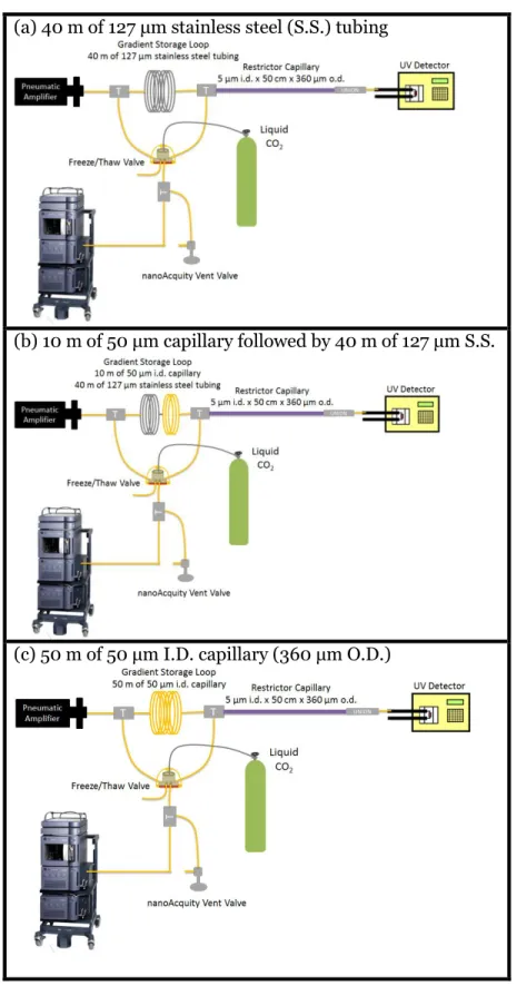
between trials. ... 110 Figure 3.12 Gradient storage loop experimental setup (1) the loop
consisted of 40 m of 127 μm stainless steel tubing (2) 10 m of 50 μm capillary follow by 40 m of 127 μm of stainless steel
tubing and (3) 50 m of 50 μm capillary tubing... 111 Figure 3.13 Setup 1 (Pin valve configuration) and Setup 2 (FT valve
implemented). ... 112 Figure 3.14 Workflow for sample processing. A sample of 0.5 mg of
xviii
fractions for protein digestion. Once back in solution, these 10 fractions underwent in-solution protein digestion. Final fractions were processed using Setup 1 and Setup 2 outlined in
Figure 3.13. ... 113 Figure 3.15 Implementation of the bleed valve to slowly release the
pressure from the system. The outlet of the bleed valve consisted of 1 m of 20 μm I.D. capillary (not shown to scale in
figure). ... 114 Figure 3.16 Temperature recorded for the copper cup placed on top of the
thermoelectric heater with varying power applied... 115 Figure 3.17 Freeze thaw valve configurations. (a) FT valve serving as a
support for the high pressure isolation valve, (b) FT valve replacing the high pressure isolation valve, and (c) FT valve replacing both the high pressure isolation valve and the high
pressure vent valve. ... 116 Figure 3.18 Comparison chromatograms for 4 configurations: (a) FT valve
replaces two pin valves as in Figure 3.17c (b) FT valve replaces the high pressure isolation valve as in Figure 3.17b, (c) FT valve is placed behind the high pressure isolation valve as in Figure 3.17a, (d) and only mechanical pin valves are utilized as
in Figure 3.1. Analyte is a BSA digest. ... 117 Figure 3.19 Organic gradient profiles: (a) 40 m of 127 μm stainless steel
gradient storage loop, (b) 10 m of 50 μm capillary followed by 40 m of 127 μm stainless steel gradient storage loop, and (c) 50 m of 50 μm capillary. The organic mobile phase (acetonitrile) was spiked with 10% acetone and monitored with UV at 265 nm. An open tubular restrictor capillary (5 μm i.d. x 50 cm)
was used in place of the column. ... 118 Figure 3.20 The gradient profiles compared for the 30 μL gradient volume.
The expected elution time for a 30 μL gradient volume was
~100 min. ... 119 Figure 3.21 Example chromatogram from two experimental designs.
Setup 1 consisted of the prior instrumental design containing three mechanical pin valves and a gradient loop consisting of 10 m of 50 μm capillary followed by 40 m of 127 μm stainless steel tubing. Setup 2 consisted of the FT valve replacing two mechanical pin valves and a gradient storage loop of 50 m of
50 μm capillary. ... 120
xix
capillary followed by 40 m of 127 μm stainless steel tubing. Setup 2 consisted of the FT valve replacing two mechanical pin
valves and a gradient storage loop of 50 m of 50 μm capillary. ... 121
Figure 3.23 Venn diagrams comparing results from Setup 1 (red) and Setup 2 (black). Proteins and peptides identified in both configurations are displayed in gray. Proteins/peptides were identified as “membrane” if they were in any way associated with the cell membrane according to the UniProKB/Swiss-Prot
protein sequence database. ... 122 Figure 3.24 The ratio of the percent coverage for the FT valve/Pin valve vs.
protein molecular weight (Da). Data above the line (45 data points) had higher percent coverage when analyzed on Setup 2 (FT valve system), and below the line (17 data points) in Setup
1 (Pin valve system). ... 123 Figure 3.25 Release of pressure over time for bleed valve. Pressure values
were obtained via flow rate measurements. ... 124 Figure 4.1 Scheme for trypsin immobilization onto BEH particles adapted
from Ahn, et al.33 (Step 1) The primary amine from the enzyme forms a temporary Schiff base with the crosslinker
triethoxysilyl butyraldrhyde. This is immediately reduced in the presence of sodium cyanoborohydride. (Step 2) The enzyme-crosslinker complex is then introduced to the BEH (5
μm, 300 Å) particles.. ... 155
Figure 4.2 Scheme for trypsin immobilization onto BEH particles via the revised (UNC) protocol. (Step 1) The BEH particles are exposed to the crosslinker which undergoes hydrolysis and condensation reactions binding to the particle surface. (Step 2) The particle-crosslinker complex is exposed to the enzyme (trypsin) and is reduced. This reaction occurs in ammonium
bicarbonate (ABC). ... 156 Figure 4.3 Reaction of Nα-Benzoyl-L-arginine ethyl ester (BAEE) with
trypsin producing Nα-benzoyl-L-arginine (BA) and ethanol. This reaction is monitored at 253 nm where the absorbance
changes 0.001 per minute. ... 157 Figure 4.4 Example of change in absorbance over time for a sample
containing trypsin (green) and without trypsin (BAEE Blank, blue). The slopes of these lines are then substituted into
equation 4-1. ... 158 Figure 4.5 Standard workflow for experiments utilizing a 15 hr in-solution
xx
mass. The equal mass fractions are digested in solution with trypsin and the resulting peptides are analyzed in the second dimension on the UHPLC instrumentation described in Chapter 3. Proteins are identified using software provided by
the manufacturer. ... 159 Figure 4.6 IMER experimental workflow. The IMER was placed after the
protein separation column via a valve so that both experiments (on-line IMER digestion and off-line IMER in-solution
digestion) could be easily compared. ... 160 Figure 4.7 Experimental setup for determining which protocol provided
the most active trypsin immobilized particles. Particles were
centrifuged prior to injection of supernatant. ... 161 Figure 4.8 Samples containing BAEE and BA were easily separated on the
PLRP-S reversed phase column using the gradient outlined in Table 4.1. Peak identities were confirmed via standard
solutions. ... 162 Figure 4.9 Example calibration curve for BCA protein assay. The blue
data points represent a series of calibrants consisting of free (unbound) trypsin in solution at various concentrations. The red data point is from a sample of immobilized trypsin particles in a slurry. This assay determined the amount of
protein (trypsin) present on the particles. ... 163 Figure 4.10 Experimental setup for determining possible flow rates
through the IMER. The effluent from the IMER
preconcentrates onto the PLRP-S reverse phase column. The valve is then switched and a gradient is run to separate any BA
from BAEE. ... 164 Figure 4.11 Experimental setup for determining the effect of organic
mobile phase on IMER digestion. BAEE was injected and sent through the IMER in a variety of organic mobile phase
compositions (Table 4.2). Gradient for the reverse phase separation is shown in Table 4.1 and the actual organic content
of the combined mobile phases is shown in Table 4.6. ... 165 Figure 4.12 Gradient profile for separation of proteins on the first
dimension reverse phase column. For yeast cell lysate analysis, mobile phase A consisted of 80% water, 10%
isopropanol, 10% acetonitrile, and 0.1% TFA. Mobile phase B
consisted of 50% isopropanol, 50% acetonitrile, and 0.1% TFA. ... 166 Figure 4.13 UV absorbance trace of analysis with (black) and without (red)
the IMER on-line. The fractions combined after lyophilizations are segmented via the red lines. Although 15 fractions were initially combined over the entire run (gradient and wash),
xxi
Figure 4.14 Slurry of trypsin immobilized particles from revised (blue) and published (red) digestion of BAEE for 1 min compared to free unbound trypsin in-solution (purple). The bottom (black) trace is a blank of BAEE solution that underwent the same protocol without trypsin present. Collected utilizing the setup
described in Figure 4.7. ... 168 Figure 4.15 BAEE injected onto the IMER with variable buffer flow rates.
The effluent of the IMER was preconcentrated directly onto the PLRP-S column (Figure 4.10) and analyzed for the presence of BA by UV detection. As shown, only a small
amount of BAEE was observed at 1 mL/min. ... 169 Figure 4.16 Comparison of organic content on IMER digestion efficiency.
BA elutes at ~6 min and BAEE elutes at ~17 min. ... 170 Figure 4.17 BA and BAEE standards injected onto the PLRP-S column
without IMER exposure. Standards were injected in a variety of organic mobile phase compositions to verify peak
placement. ... 171 Figure 4.18 Venn diagram comparing the proteins identified with (green)
and without (blue) the IMER on-line: (a) total protein
identifications and (b) membrane protein identifications. ... 172 Figure 4.19 The proteins identified by both the IMER and in-solution
digestions plotted (a) by molecular weight and (b) by
isoelectric point. ... 173 Figure 4.20 The percent coverage for the 370 total proteins identified by
both the IMER (green) and in-solution (blue) digestions
plotted against molecular weight... 174 Figure 4.21 The ratio of percent coverage found in the 370 total proteins
and 94 membrane proteins identified by both the IMER and in-solution digestions. The ratio was IMER/in-solution, therefore positive values indicate the IMER digestion had a higher percent coverage than the in-solution digestion and negative values indicate the in-solution percent coverage was
higher. ... 175 Figure 5.1 Multidimensional proteomic workflow resulting from IMER
implementation. The fractions are collected off-line and
lyophilized followed by UHPLC-MS analysis. ...205 Figure 5.2 Comparison between fully automated on-line digestion and
MS/MS application. ... 206 Figure 5.3 Configurations for interfacing IMERs for separation and
xxii
represents a two-dimensional analysis. Image adapted from
Ma, et al.6 ... 207 Figure 5.4 Fully automated RPLC-IMER-RPLC-ESI-MS on-line digestion
workflow. ... 208 Figure 5.5 Experimental protocol for determining the actual residence
time of model proteins BSA, RNAse A, myoglobin, and cytochrome C. (a) Proteins were injected, digested on-line, and collected into 5 fractions. These fractions were not lyophilized, but were injected on a standard ESI-MS for protein detection. Flow rate through the IMER was 0.5 mL/min. (b) Proteins were injected, digested on-line, and preconcentrated directly onto a second-dimension reverse
phase column for ESI-MS detection. ... 209 Figure 5.6 Configurations for monitoring dispersion due to IMER
implementation: (a) no IMER present (b) IMER placed after
separation column to determine dispersion effects. ... 210 Figure 5.7 Method for off-line multidimensional workflow with
in-solution digestion. This was a fair comparison to the on-line multidimensional IMER workflow since it utilizes the same
first and second-dimension columns and flow rates... 211 Figure 5.8 Detection of proteins over time after eluting from the IMER at
0.5 mL/min. Fractions were collected as depicted in Figure
5.5a. ... 212 Figure 5.9 Results for percent coverage and number of digest peptides for
BSA and myoglobin while varying the concentration injected on the IMER. Data was collected using the configuration
outlined in Figure 5.5b. ... 213 Figure 5.10 Monitoring peak dispersion through IMER using model
substrate BAEE and hydrolysis product BA. ... 214 Figure 5.11 Protein elution on the PLRP analytical column with an
extended first-dimension gradient. Four standard proteins were injected (RNAse A, cytochrome C, BSA, and myoglobin) to determine if the two-dimensional setup was operational. The gradient was extended so that the proteins would be
separated on the second-dimension alternating columns. ... 215 Figure 5.12 Second-dimension base peak intensities (BPIs) from injection
of four standard proteins (RNAse A, cytochrome C, BSA, and
myoglobin) onto the LC-IMER-LC-MS workflow. ... 216 Figure 5.13 Summed peptide intensity for four standard proteins (RNAse
A, cytochrome C, BSA, and myoglobin) plotted against
xxiii
Figure 5.14 Second-dimension peptide separations from 0.25 mg of yeast cell lysate. Each second-dimension run was 20 min (not shown on axis). It is plotted aligning with the second-dimension run, such that peptides which eluted between 20-40 min (y-axis) eluted during run 1, 20-40-60 run 2, 60-80 run 3, etc. The first-dimension gradient profile is overlaid on the x and y axes. The x-axis corresponds to the first-dimension gradient (percent organic) during which the peptides would elute to the second-dimension. For example 0-7%B would
correspond to run 1, 7-15% run 2, 17-20% run 3, etc. ... 218 Figure 5.15 Number of unique protein identifications plotted versus
second-dimension run number. ... 219 Figure 5.16 Proteins identified for 0.25 mg insoluble portion of a yeast cell
lysate plotted vs. (a) percent coverage, (b) molecular weight,
and (c) isoelectric point. ... 220 Figure 5.17 Total protein identification results for the 0.25 mg sample for
the IMER (green) and the in-solution (blue) digestions. ... 221 Figure 5.18 Proteins identified for 0.5 mg insoluble portion of a yeast cell
lysate plotted vs. (a) percent coverage, (b) molecular weight,
and (c) isoelectric point. ... 222 Figure 5.19 Total protein identifications for the 0.5 mg sample injected for
the IMER (green) and the in-solution (blue) digestion. ... 223 Figure 5.20 For the 46 commonly identified proteins for the 0.5 mg sample
injected (a) the log of the ratio of the percent coverage vs. molecular weight and (b) the log of the ratio of the summed
xxiv
LIST OF ABBREVIATIONS AND SYMBOLS
% A percent aqueous mobile A (aqueous) % B percent mobile phase B (organic)
2D two dimensional
ABC ammonium bicarbonate
BA Nα-benzoyl-L-arginine
BAEE Nα-benzoyl-L-arginine ethyl ester
BCA bicinchoninic acid
BEH bridged ethyl hybrid
BPI base peak intensity
BSA bovine serum albumin
CE capillary electrophoresis
CHAPS 3-[(3-cholamidopropyl)dimethylammonio]-1-propanesulfonate CID collision induced dissociation
cm centimeter
CZE capillary zone electrophoresis
DC direct current
Dm diffusion coefficient in the mobile phase
dp particle diameter
DPDT double pull double throw
ECD electron capture dissociation
ε mobile phase fraction
εi interparticle porosity
ESI electrospray ionization
xxv
FA formic acid
FASP filter-aided sample preparation
FT freeze/thaw
FTICR Fourier transform ion cyclotron resonance mass spectrometry
γ tortuosity factor
H height equivalent to a theoretical plate HPLC high-pressure liquid chromatography ICATs isotope-coded affinity tags
I.D. internal diameter
IEF isoelectric focusing
IMER immobilized enzyme reactor
IPI International Protein Index
λ geometric factor
LC liquid chromatography
M molar
m/z mass to charge ratio
MALDI matrix assisted laser desorption ionization
μm micron
mg milligram
min minute
mL milliliter
mm millimeter
MOSFET metal oxide semiconductor field effect transistor
MS mass spectrometry
MSE mass spectrometry expression
xxvi
MudPIT Multidimensional Protein Identification Technique
N number of theoretical plates
nc peak capacity
NCBI National Center for Biotechnology Information
nL nanoliter
nm nanometer
NPT National pipe thread
O.D. outer diameter
P pressure
PAGE polyacrylamine gel electrophoresis
PEEK polyether ether ketone
pI isoelectric point
PLGS Protein Lynx Global Server
PLRP polymeric reverse phase
psi pounds per square inch
PTFE polytetrafluoroethylene
PTMs post translational modifications Q-TOF quadrupole time-of-flight
r radius
RP reverse phase
SAX strong anion exchange
SCX strong cation exchange
SDC sodium deoxycholate
SDS sodium dodecyl sulfate
sec second
xxvii
SILAC Stable Isotope Labeling by Amino acids in Cell cultures SOP standard operating procedure
SQ % percent sequence coverage
TFA trifluoroacetic acid
tg separation window
TPCK tosyl phenylalanyl chloromethyl ketone
u mobile phase linear velocity
UHPLC ultra-high pressure liquid chromatography
UV ultraviolet
V volt
WAX weak anion exchange
1
CHAPTER 1. Introduction to Membrane Proteomic Analysis Using
Multidimensional Liquid Chromatography – Mass Spectrometry
1.1 Introduction to Proteomics
The basic functions of biological systems are controlled by extremely complex gene
expression and the resulting activities of their protein products.1 Proteins consist of one or more
long chains of amino acids and are responsible for vital cellular activities. Proteins act as catalytic enzymes, take on a regulatory role for gene expression, provide cellular structural
components, and act as messengers within and between cells.2, 3 The importance of these roles
makes the identification of proteins beneficial to a wide range of disciplines; ranging from
fundamental biological studies, pharmaceutical development,4 to clinical diagnostics.1
Proteomics is defined as the study of multiprotein systems in an organism and how these systems can change with time and condition. The entirety of proteins that can be expressed by an organism is termed the proteome. A major challenge in proteomics is the dynamic nature of
the proteome itself. It can be expected that different cells (i.e. from different tissues) can
express different proteins; however, the same cells may also express different proteins
depending on the stage of the cell. The stage of the cell can be interpreted as the lifecycle of the cell or the response of the cell to the state of the organism (for example a diseased state). Therefore the proteome is defined by the state of the organism, tissue type, or cell where it
originates. Since these states are constantly changing, so are the proteomes themselves. Adding
another level of complexity, the proteins within the system can exist in multiple forms
2
the protein lifecycle can involve distinct modifications to the protein structure. A single protein can carry multiple modifications, and each modification can be permanent or transient, all of
which add additional levels of complexity to the system under study.1, 3 The degree to which a
protein can be modified varies based on regulatory mechanisms within the cell, environmental factors (drugs/chemical influences), and the protein itself. The overall result is any protein can
be present in multiple forms at any time within a cell, presenting a large analytical challenge.1
1.2 Membrane Proteins
Although cytosolic proteins are the easiest to identify due to their solubility, most cell signaling proteins are associated with the membrane. The hydrophobic nature of membrane proteins, which contributes to the difficulty of their extraction and analysis, is mainly due to the
α-helices that traverse the bilayer (~15-25 amino acids in length).5, 6 It has been estimated that
transmembrane proteins constitute ~30% of the total proteins within a cell.7 While certain
proteins are strongly hydrophobic and intrinsic to the membrane, others are more amphipathic and merely membrane associated. Membrane proteins lie in junctions between cells and intracellular components where they mediate communication and control cell adhesion for tissue formation. In addition, membrane proteins dictate immune response recognition, metabolic processes, vesicle trafficking, ion transport, protein translocation/ integration, and
propagation of signaling cascades.4, 8 These cellular ―doorways‖5 are extremely important for
pharmaceutical drug targeting,4 including G-protein coupled receptors and cytochrome p450s.6
Despite their usefulness, these proteins are difficult to extract and analyze from their native hydrophobic environment. Membrane proteins often precipitate during sample handling, are not soluble in commonly used solvents, and tend to transfer contaminants such as lipids from their native environment during their extraction from the cell. Because of the difficulty involved and the importance of working with membrane proteins, there are multiple suggested
3
multiple sample techniques for all four stages of sample preparation including cell lysis, protein enrichment, solubilization, and digestion, for membrane proteomic analysis.
1.3 The Tools of Proteomics
Since the phrase was coined by Wilkins in 1990, ―proteomics‖ has expanded far beyond
the Western blots and Edman degradations of its beginnings.1, 3 The modern proteomic toolbox
(Figure 1.1) consists of four areas: sample preparation, chromatographic separation, mass spectrometry (MS), and data analysis. Accurate protein identification relies heavily on all four areas, and improvement in any one aspect will enhance the capabilities as a whole. Thus the focus of this dissertation was to develop improved methods for sample preparation and chromatographic separations for biologically complex membrane protein mixtures.
In order to measure the efficiency of a gradient separation, peak capacity (nc) is used.
The peak capacity is defined as the number of peaks that can be resolved in a defined separation
window9, 10 and is given by the formula:
(1-1)
The separation window (tg) can be defined as the gradient time or the time between the
first and last eluting peak. The peak width (or average peak width) is determined at the width
4σ, which corresponds to 11% of the maximum peak height and is defined for two overlapping
adjacent peaks having a resolution of 1 (unit resolution).11 Thus, the greater the peak capacity,
the more analytes can be resolved successfully and ultimately identified within a specific time frame.
The overall goal of any separation technique is to develop a method to detect a large number of distinct molecular species. This is especially difficult for proteomics, for which most species of interest are at low levels and exist in various modified forms. Due to the complex nature of protein mixtures, proteins and peptides are separated using high resolution
chromatographic techniques.1 With high resolution techniques, the goal is to reduce the number
4
can be performed on proteins as a whole or after digestion, both of which take advantage of the
differences in physical properties.1 Protein properties commonly exploited for separations in
proteomics include size, charge, hydrophobicity, and affinity.13 When mass spectral detection is
performed on the intact protein the method is referred to as top-down and typically requires expensive high resolution mass spectrometers. More commonly, the proteins are digested into peptides (bottom-up) and these smaller fragments are detected and compared to a proteomic database for protein identification. The digestion is primarily performed with the enzyme trypsin due to its specificity. A typical protein might have approximately 30 tryptic peptides (each peptide typically consists of 10-15 amino acids) and there are on average 10-12 thousand
proteins expressed in a human cell.12, 14-16 The result of a bottom-up experiment is
differentiating a large number of peptides, which can lead to a complex sample with numerous analytes requiring high resolution separation strategies. Common types of separation and detection techniques are described below for both protein and peptide analyses.
1.3.1 Separation Techniques
Despite the high resolution of mass spectrometers, in order to fully understand the biologically complex system of the proteome, the mixture must be separated prior to detection. Traditional protein separation methods such as polyacrylamine gel electrophoresis (PAGE), high-pressure liquid chromatography (HPLC), capillary electrophoresis (CE), and isoelectric focusing (IEF) are common along with more modern approaches involving more than one separation technique in tandem. The latter, referred to as a multidimensional analysis, was a
major breakthrough in protein and peptide separations.1
5
components.17 Precipitation becomes even more problematic with hydrophobic/non-polar
proteins (such as membrane proteins), which tend to form insoluble complexes and precipitate
prior to loading.3 Despite difficult protein recovery from the gel matrix18 and incomplete
resolution for complex samples,19 2D-PAGE remains the gold standard compared to more
current protein separation strategies.13
High pressure liquid chromatography (HPLC) is an attractive alternative to 2D-PAGE due to its high resolving power, reproducibility, various commercially available stationary
phases, and compatibility with electrospray ionization mass spectrometry (ESI-MS).20 Out of
the multiple modes of analysis available for separation, reverse-phase (RP) HPLC is most
utilized because of solvent compatibility (polar) with protein/peptide dissolution.21 Greater
than 98% protein recovery and reproducibly high resolution have been reported using high
temperature RP macroporous columns for intact protein analysis.22 Additional modes
commonly used for protein separation include size exclusion chromatography (SEC), affinity chromatography, and ion exchange chromatography.
Size exclusion chromatography is used to purify, estimate molecular weight, and study interactions between proteins. While SEC can separate proteins based on size and aid in
identifying protein folding, structure, and stability,23 the low resolution of SEC makes it less
desirable than reverse phase or ion exchange. Another common method of protein purification is affinity chromatography, which separates proteins based on specific physical interactions
between an immobilized ligand and binding partner in order to retain compounds of interest.3
Typically the ligands utilized for affinity chromatography consist of antibodies. Due to its use of antibodies, this technique can be extremely expensive and typically is used to specifically target
analytes of interest (such as analytes with specific PTMs).13 A major contributor in protein
6
negatively charged sulfonic acid modified surface. The positively charged peptides interact with the column with a strength dependent on their respective charge. A salt solution or pH gradient is applied to the column to compete for charge sites or alter the protein/peptide charge state for
elution, respectively.3, 12 Previous work in the Jorgenson lab, investigated protein separation
with ion exchange and reverse phase.24 When the sample was separated by reverse phase, 546
proteins were identified compared to only 262 with anion exchange. Therefore, reverse phase separation of proteins became the standard procedure for the proteomic workflow in our lab (Figure 1.2).
As expected, the separation of intact proteins (vs. peptides) has the advantage of producing a less complex sample. However, there is limited information that can be obtained from this approach and traditionally protein digestion into peptides is preferred for large scale
proteomic analyses.2 Digestion of the protein prior to separation is advantageous since peptides
are generally more soluble than their intact protein counterparts. On the other hand, the mixture is now more complex, as there are more species to resolve and the protein of origin for
ambiguous peptide sequences (along with cleaved PTMs) are difficult to determine.12 The
increased solubility of peptides in common RP solvents, high resolution, and the amenability of RP chromatography to ESI-MS detection make it the most prevalent mode of separation for peptide analysis. Thus, in the proteomic workflow presented in Figure 1.2, this mode is also employed for peptide separations.
1.3.2 Mass Spectrometry
Today, protein and peptide detection is primarily performed via mass spectrometry. Popular ionization techniques to obtain mass spectra of large biological molecules include electrospray ionization and matrix assisted laser desorption ionization (MALDI). ESI is what initially allowed HPLC to be directly coupled to MS, with the effluent of the HPLC column being
continuously ionized.21 Ions for ESI are produced as the sample flow stream is passed over a
7
that are in aqueous solution exist as ions because they contain certain functional groups whose
ionization is controlled by the pH of the solution.25 The ions produced by this process are then
desolvated by either heat or nitrogen gas and as the droplets become smaller, the increasing electric field causes the analytes to desorb from the surface. The resulting desolvated analyte ions are fed into the MS under vacuum. Ultra-low flow sample inlet systems for ESI, termed nanospray (50-500 nL/min), allow for more efficient transfer of ions (lower limits of detection) from solution to the mass analyzer. ESI is applied extensively in top-down protein and
bottom-up peptide proteomic analyses.1, 3
Types of mass analyzers that are typically used for proteomics include time-of-flight (TOF), quadrupole filters, orbitraps, and ion cyclotron resonance. Combining two or more mass analyzers in tandem allows the investigator to select a precursor ion of interest and subject it to further fragmentation in a collision cell followed by detection. Subjecting the ion of interest to further fragmentation provides additional structural information for the analyte. For tandem
MS (designated as MS/MS), the first mass analyzer selects a specific m/z range. These ions
undergo fragmentation and the resulting fragments are measured according to their m/z by a
second mass analyzer.3 When ESI is paired with tandem MS, the resulting mass analyzers are
typically a triple quadrupole, an ion trap (MSn), or a quadrupole-time of flight (Q-TOF).1
In a tandem proteomic MS analysis, the two most common fragmentation methods are collision-induced dissociation (CID) and electron capture dissociation (ECD). For CID, a collision cell with an inert gas builds potential energy with repeated collisions of the analyte ion until the ion reaches a threshold and fragments. For proteins and peptides, CID generally targets weak noncovalent bonds, covalent bonds responsible for PTMs, and the peptide bond.
The fragment ions are then analyzed based on their m/z and an ion spectrum is produced.1
8
cleavage site, rearrangements are minimized and cleavage of the backbone is favored over the noncovalent bonds (weak noncovalent bonds and hydrogen bonds) responsible for secondary and tertiary conformational structure of protein ions. Since the conformational bonds are less likely to be broken, ECD is useful in providing primary structure as well as studying secondary
and tertiary structure of protein ions.26 For peptide analysis, ECD is useful for preserving PTMs.
A type of MS that utilizes ECD fragmentation is Fourier transform ion cyclotron resonance mass
spectrometry (FTICR-MS).27 FTICR-MS is the preferred method for accurate mass
measurements of intact proteins, detecting masses with extremely good mass accuracy (~0.5-1
ppm).28 The advantages of this technique include sensitivity, dynamic range,
comprehensiveness, and throughput.4, 29 However, FTICR mass spectrometers are expensive to
purchase and maintain. Alternatively, protein identifications can be performed via bottom-up analyses with less costly equipment. With a bottom-up approach, at times only a single peptide is required to identify a protein and competitive ionization of analytes can be decreased if high
resolution capillary chromatography (nano-LC) with ESI is applied.20
The type of mass analyzer used for the research presented here is the Waters Q-Tof
PremierTM. This type of instrument performs parallel alternating scans which are acquired at
either low or high collision energy. This process of simultaneously collecting parent and
product ion spectra is referred to as MSE. MSE maximizes the instruments duty cycle by rapidly
switching between low and high collisional energy, producing alternate precursor and fragment
ions to maximize data collection efficiency. 30, 31, 32 MS/MS is a serial approach to interrogating
ions, which switches between observing all precursor masses within a range and selecting the
most intense for sequential fragmentation scans. In contrast, MSE fragments all precursor ions
with a continuous unbiased approach. Overall, MSE is a robust way to obtain qualitative and
quantitative data and has provided enhanced protein sequence coverage and higher quality
9
MS quantification includes isotopic labeling and label-free techniques. A metabolic labeling process referred to as SILAC (Stable Isotope Labeling by Amino acids in Cell cultures) is
commonly used in vitro. This technique labels the peptide with stable isotopic nuclei 2H, 13C,
15N and is commonly used to study PTMs. 31, 34 Chemical and enzymatic tags are also used for
peptide and protein labeling.34 Isotope-coded affinity tags (ICATs) is a chemical technique that
takes advantage of differential tagging of cysteine residues by affinity and ion-exchange
chromatography. As a way to avoid sample modification, label-free quantification monitors an internal standard, such as BSA (bovine serum albumin). By entering the known quantity of a standard into the MS software, certain instruments will monitor the spectral counts from the internal standard and report amounts of proteins and peptides based on a relative comparison. Label-free quantification has been well documented in the literature as a valid method of
quantification with lower cost and reduced sample modifications.35, 36
Once spectral data is obtained, computer algorithms are utilized to quickly identify the protein mass and identity. For top-down experiments, deconvolution algorithms report the protein mass. In bottom-up experiments, the protein is identified by comparing the amino acid sequence to a proteomic database. There are many theoretical and known peptide masses in established databases, with the most common being UniProt, Swiss-Prot, TrEMBL, National Center for Biotechnology Information (NCBI), and International Protein Index (IPI). Vendor software using data reduction algorithms help the user select parameters for database searches. Information such as the number of possible missed cleavages, enzyme used to cleave the
proteins, and description of possible PTMs can be taken into account with the software. For example, a typical modification that occurs during tryptic digestion is the reduction and
alkylation of cysteine thiols with iodoacetamide or iodoacetate. This results in cysteine residues that may contain different masses and including such a possibility in the search can greatly
improve the confidence of the reported match. Once a tolerance of m/z values is selected, the
10
resulting database hits are then subject to calculation of match scores for user comparison. Scoring is typically based on the intensity of the ion, the number of peptides detected, and pattern of fragmentation compared with the database. How well a protein sequence is
represented by MS data is referred to as protein coverage.3 Typically 20-40% sequence coverage
is experimentally obtained and statistics and confidence intervals are based on the calculated
coverage.3
1.4 Multidimensional Separations
To further decrease the complexity of proteomic samples, multidimensional separation techniques are employed. In these configurations, a sample is subjected to more than one type of separation. A common example of this is 2D-PAGE, where a sample is first separated by isoelectric point and then by size. Since these two separation characteristics (isoelectric point and size) are not directly related, these techniques are considered orthogonal and should give
optimal separation efficiency.3 Multidimensional analyses apply two or more orthogonal
separation techniques in tandem.13 According to Giddings’ criteria for an ideal two dimensional
system, the separations must be orthogonal and resolution gained in the first dimension cannot
be lost in the second dimension.25, 37 Relying on two or more independent techniques,
multidimensional analysis provides a better separation than either single dimension alone would allow. Ideally, the resulting peak capacity is the product of the peak capacities for the
individual methods, albeit difficult to achieve in practice.13 A multidimensional analysis
performed by Link, et al. utilized SCX and RP prior to MS analysis. The authors directly compare proteins identified using one dimensional and two dimensional LC techniques. Overall, 3.5 times more peptides and 1.7 times more proteins were identified by subjecting the
analytes to separation in a second dimension.38
11
the first dimension and stored for later application onto the second dimension.12, 37
Comprehensive on-line techniques have the additional challenges of solvent compatibility between dimensions, band broadening in valves/loops, and a need for a second dimension that
is faster than the first.39 Although on-line techniques are faster than off-line, there are less
mobile phase restrictions for off-line methods.12, 37 The goal of the overall experiment, whether
it be speed, protein recovery, or better resolution, will determine which technique is applied. The original off-line multidimensional approach utilized in the Jorgenson lab is shown in Figure 1.2. Although reverse phase chromatography is employed in both dimensions, orthogonality
was demonstrated due to the enzymatic digestion between the first and second dimensions.24
Aside from 2D-PAGE, among all the combinations of separation modes reported in the literature, ion exchange chromatography (specifically strong cation exchange) coupled with RP-HPLC is the most common for protein and peptide analysis. Because RP-RP-HPLC utilizes
stationary phases that allow for high optimum flow rates and mobile phases that align with MS, it is commonly placed in the second dimension due to the capability of fast sampling speeds and
detector compatibility.1 The most familiar configuration of this setup is MudPIT or
Multidimensional Protein Identification Technique.1, 13, 6, 8 Unique to MudPIT, the two stationary
phases (SCX and RP) are packed sequentially into a single microcapillary column, of which the
tip is pulled for direct ESI coupling.37 Digested peptides are first subjected to SCX in which the
peptides adsorb with affinities proportional to the overall number of positive charges and elute in a step gradient of increasing salt concentration. Each step in the gradient releases a group of peptides that pass onto a RP column, where the peptides are separated based on hydrophobicity and analyzed by MS. This tandem approach not only aids in providing better separation, but
also allows for low-abundance proteins to be identified.1, 13, 29 MudPIT is an unbiased, biphasic,
online 2D-LC/MS/MS system2,11 that has been capable of identifying over 1,000 proteins in a
12
only modes applied to MudPIT (due to gradient restrictions), it has been suggested that a
three-phase MudPIT column with an additional RP can further improve separation.37
Although ion-exchange is most often coupled with RPLC, other two dimensional combinations can include affinity-RPLC, SEC-RPLC, and RP-capillary zone electrophoresis
(CZE).20, 40 Hypothetically, any of the separation modes described to separate peptides and
proteins can be linked in two dimensional analysis; however, by doing so the instrument becomes increasingly more complex. The differences in pressure, run time, gradient phases, and peptide solubility between modes can make operation difficult. Thus, column-switching valves have proved valuable to multidimensional separation, providing better flexibility than directly coupled systems. Described by Bushey and Jorgenson in 1990, a comprehensive system for LC was used to analyze protein mixtures with a SCX coupled to SEC in the second dimension via an eight port switching valve. The valve was designed to switch between the storage loop,
columns, pump, and waste with computerized control.37
When considering off-line multidimensional techniques, prefractionation is suggested
for cleaner mass spectra and better chromatographic separation.12, 14, 15 Instead of complete
separation and analysis of proteins or peptides on multidimensional systems, intact proteins can be prefractionated, digested into peptides, and introduced to a second analytical separation. These hybrid techniques take full advantage of the different physiochemical characteristics between proteins and peptides. However, deciding on the number of protein fractions to collect in the first dimension is crucial. Too many fractions increase experimental time and labor, while
too few fractions do not reduce sample complexity as desired.22 The optimal number of
fractions depends on many things, such as the complexity of the sample, sample size, gradient, available experimental time, MS mode, and the purpose of the analysis. Although fractions anywhere from 5 to 20 are typical, up to 96 fractions have been reported for a complex protein
13
1.5 Fully Automated On-line Proteomic Workflows
Recently, efforts have been made to include proteomic sample preparation steps in multidimensional workflows. Off-line aspects of a bottom-up analysis, typically performed prior to chromatographic separation, include protein reduction, alkylation, and in-solution enzyme digestion. By implementing these steps into an automated multidimensional scheme, one reduces the potential for sample contamination and sample loss, speeds up the analysis, and provides the ease of automation. One major area of interest for employing on-line digestion is Immobilized Enzyme Reactors (IMERs). These reactors contain immobilized enzyme on a substrate. The substrate can consist of a variety of materials for diverse applications (described in more detail in Chapter 4); however, one of the more common configurations involves the substrate in a chromatography column for rapid flow-through on-line digestion of the protein sample.
Ideal protein digestion cleaves at specific amino acids, providing fragments suitable for MS analysis (6-20 amino acids) and database comparisons. A few of the proteases available for protein digestion are trypsin, chymotrypsin, Lys C, and Asp N. Trypsin is the most widely used since it has high specificity, produces peptides of suitable length, and is easily purified from porcine or bovine pancreata. Trypsin cleaves proteins at lysine and arginine residues unless
either amino acid is followed by proline in the C-terminal direction.1, 3 Although IMERs can be
developed from a multitude of enzymes, trypsin is the most popular. IMER columns have been
developed for microfluidic devices42, on a capillary scale43, and in more traditional standard bore
chromatography columns (2.1-4.6 mm).44 The standard bore columns usually consist of a
monolithic material or a particle packed substrate with trypsin immobilized. These columns are highly successful at protein digestion due to the high enzyme to substrate ratio, with low trypsin autolysis products, and reduced missed cleavages. Placing these columns in an on-line
14
of such an IMER to our multidimensional proteomic workflow is described in Chapter 4. A level of difficulty arises when attempting to perform a fully automated multidimensional proteomic analyses with on-line digestion. Obstacles such as solvent compatibility, pH requirements for digestion and ionization, and preconcentration of peptides in the second dimension are not trivial to overcome. Chapter 5 outlines a fully automated on-line multidimensional workflow involving IMER on-line digestion for proteomic analysis of membrane proteins.
1.6 Introduction to Ultra High Pressure Liquid Chromatography
The development of Ultra High Pressure Liquid Chromatography (UHPLC) by the
Jorgenson group45 has been a major advancement for the separation of proteomic samples,
doubling the peak capacities achieved with standard HPLC. Using the same column, faster flow rates can be achieved at higher pressures (Figure 1.4) which reduces analysis time. The ability to work at higher pressures also allows for the use of longer chromatographic columns (~1 m),
which increases separation space (Figure 1.5), and smaller diameter stationary phases (dp < 2
μm), which increases efficiency. These gains in efficiency are demonstrated by the simplified van Deemter equation below:
A
or (1-2)
dp 2 u m u dp
2
6 m
Where is the geometric factor, dp is the particle diameter, uis the mobile phase linear
velocity, is the tortuosity factor, and Dm is the diffusion coefficient in the mobile phase. The A,
B, and C terms are van Deemter coefficients that describe band broadening contributions from eddy dispersion, longitudinal diffusion, and resistance to mass transfer, respectively. The height equivalent to a theoretical plate (H) and number of theoretical plates (N) are parameters used to determine and compare column efficiency.
15
By increasing the number of theoretical plates (N), and as a result decreasing the size of the height equivalent of a theoretical plate (H), there is an observed increase in efficiency. As
expressed in the equations above, by decreasing the particle size (dp) or increasing the length (L)
of the column, this is accomplished. However, this gain in efficiency with smaller particles and longer columns is not without a cost as there are practical and instrumental limitations.
Practically, users want to perform the best analysis possible in the shortest amount of time, and longer columns with smaller particles on a commercial system (limited to ~10–15 kpsi) will result in low flow rates and long run times. In order to achieve the gain in performance from these long columns with smaller particle diameters, higher pressures are required to perform the analysis in a reasonable time frame.
Built in-house, the UHPLC gradient system developed in the Jorgenson lab operates at
~35 kpsi (Figure 1.6).41, 46, 47 A commercial pump is utilized to inject the sample and gradient
16
reported as percent change in organic (B) per column volume, where an aggressive gradient is considered ≥4% change in B per column volume and a shallow gradient is ≤ 1% change in B per column volume.
Overall, the advent of UHPLC greatly increased peak capacity compared to commercial systems (Figure 1.7). However, UHPLC does require external valves and specialty high-pressure fittings. Routine use over time at high pressures can also take its toll on the instrumentation, causing valves to leak and fittings to clog with heavy usage. Therefore, Chapter 3 focuses on advancements made to the UHPLC system to address such issues. This includes a high pressure valve featuring freeze/thaw technology and an improved gradient storage system, with the main goal to improve the reproducibility, longevity, and separation efficiency of the system.
1.7 Scope of Dissertation
17
18
1.8 FIGURES
19
20
21
22
Figure 1.5 Gain in peak capacity seen by implementing longer chromatographic columns, increasing the separation space for complex sample analysis. Reproduced with permission from
23
24
Figure 1.7 Comparison of three columns of different length analyzed with MassPREPTM digestion standard expression mixture 2. Due to the length of these columns the pressure was increased (~30 kpsi) using the UHPLC system. For comparison (black line) a commercial column packed with the same material (1.9 μm E 18) was used to separate the mixture at commercial pressures (~8 kpsi). Reproduced with permission from the dissertation of K.