Graph Databases and DBMSs - Free Computer, Programming, Mathematics, Technical Books, Lecture Notes and Tutorials

(1)

Université libre de Bruxelles

INFO-H-415

Advanced Databases

Graph Databases and Neo4J

Authors:

Anna

_{Turu Pi}

Ozge

_Koroglu

Supervisor:

Esteban

_Zimányi

(2)

List of Tables

1 Comparison of ACID and BASE Consistency Models . . . 13

2 Graph database schema . . . 42

List of Figures

1 Evolution of database technology . . . 7

2 DBMS marketplace . . . 8

3 DBMS developed by database model pie chart . . . 9

4 DBMS popularity by database model pie chart . . . 10

5 Four main types of NoSQL databases . . . 12

6 Positions of NoSQL databases (source: Neo4j) . . . 16

7 DBMS popularity by database model pie chart . . . 17

8 Model Comparison . . . 19

9 Query execution in graph databases . . . 20

10 Query execution in relational databases . . . 20

11 Graph DBMS Ranking . . . 21

12 Trend Graph DBMS popularity scatter plot . . . 22

13 Neo4j As a Leading Graph Database . . . 24

14 Level Of Complexity of Traditional Databases Comparing to Neo4j . 25 15 Ebay’s comment about Neo4j . . . 25

16 General Look at Neo4j . . . 27

17 Query times for Oracle Exadata vs Neo4j . . . 29

18 Tomtom’s Comparison of Neo4j with MySQL . . . 29

19 Node Representation . . . 31

20 Relationship Representation . . . 31

21 Create Person’s Node . . . 32

22 Create Relationship Between Two Nodes . . . 33

23 Relationships . . . 33

24 Match Result . . . 34

25 Delete Result . . . 35

26 Load CSV Operator Structure . . . 35

27 Use Cases Of Neo4j . . . 36

(5)

34 Example of a query in Neo4j . . . 43

35 Relational database diagram . . . 44

36 Exporting Neo4j database to CSV file . . . 45

37 CSV file containing Neo4j database . . . 45

38 Exporting Neo4j database to cypher script . . . 46

39 Cypher script containing Neo4j database . . . 46

40 Algorithms for graph databases . . . 47

41 Add jar files in plugin folder . . . 47

42 Shortest path query from Madrid to Seoul . . . 48

43 Pipeline of the shortest path query . . . 49

44 Expanded shortest path query . . . 49

45 Shortest path query from Seoul to Antwerp . . . 50

46 Neo4j DB schema after adding Connected relationships . . . 51

47 Neo4j DB schema after adding Goingto relationships . . . 52

48 Shortest path between Madrid and Seoul . . . 52

49 Shortest path outbound route output . . . 53

50 Shortest path return route output . . . 53

51 Other shortest path examples . . . 54

52 SQL Server recursive query output . . . 55

53 Neo4j query on Antwerp-Istanbul shortest path . . . 56

54 Pipeline of Neo4j query on Antwerp-Istanbul shortest path . . . 57

55 Concept of betweenness centrality . . . 58

56 Betweenness centrality query result . . . 58

57 Pipeline of the betweenness centrality query . . . 59

58 Concept of closeness centrality . . . 60

59 Closeness centrality query result . . . 60

60 Location of the airports with highest closeness centrality . . . 61

61 Pipeline of the closeness centrality query . . . 62

62 Airports pagerank result . . . 63

63 Pipeline of the airports pagerank query . . . 63

64 Airlines pagerank result . . . 64

65 Pipeline of the airlines pagerank query . . . 65

66 Community detection graph . . . 66

67 Community detection table . . . 67

68 Pipeline of community detection query . . . 68

69 Papua New Guinea partition . . . 69

70 Canada partitions . . . 69

71 Algeria partition . . . 70

72 Finland, Greenland, Iceland partitions . . . 70

(6)

74 Europe partition . . . 71

75 Australasia partition . . . 72

76 Comparison of Queries - first query . . . 74

77 Comparison of queries - second query . . . 75

(7)

1 Introduction

(8)

2 Background

The aim of this project is to prove that graph databases, more specifically Neo4j, was the most performant DBMS for some specific use cases, hence they earned their place in the DBMS’s market. The first milestone was to investigate the state of the art of DBMS. Its purpose was to justify the existence of graph databases, showing that it meets some needs not covered by other DBMS.

2.1 State of the art of Databases

Database Systems evolution: Databases and database technology are vital to modern organizations supporting both the daily operations and decision making. Database technology has undergone remarkable evolution over 50 years. Despite dominance to the enterprise DBMS marketplace by Oracle, the industry remains highly competitive with a continued high level of innovation [12].

Figure 1: Evolution of database technology

(9)

• 2nd Generation (1970’s): Navigational – Could manage multiple entity types and relationships. Computer program still has to be written. Progress on standards.

• 3rd Generation (1980’s): Relational with non-procedural access – Founda-tion based on mathematical relaFounda-tions and associated operators. OptimizaFounda-tion technology was developed. IBM performed pioneering research to enable com-mercialization of relational database technology.

• 4th Generation (1990’s+): Object oriented – Are extending the bound-aries of database technology. New kinds of distributed processing and data warehouse processing. Can store and manipulate unconventional data types. Convenient ways to publish static and dynamic Web data.

DBMS marketplace: Despite dominance to the enterprise DBMS marketplace by Oracle, with more than 40% overall market share, the industry remains highly competitive with a continued high level of innovation. In some environments, its competition is Microsoft SQL Server, IBM DB2, Teradata, SAP Sybase. Open source DBMS products have begun to challenge the commercial DBMS products at the low-end of the enterprise DBMS marketplace. The category of open-source DBMS is leaded by MySQL, followed by MongoDB, PostgreSQL and MariaDB. In the desktop DBMS market, Microsoft Access dominates because of the dominance of Microsoft Office. [12]

Figure 2: DBMS marketplace

Innovation in the industry: The advances in DBMS in recent years support business intelligence processing for data integration and usage of summary data.

(10)

horizon-global availability,easy replication support,simple API,eventually consistent/BASE (not ACID), and large scale data. [5] [19]

2.2 Types of DBMS

Ranking In this section we observe rankings created by DB-Engines. DB-Engines is an initiative that provides information on the popularity of the DBMS available in the market. They make available different rankings for every DBMS type, which are updated monthly. [3]

Figure 3: DBMS developed by database model pie chart

Over those lines, a pie chart represents the categories of DBMS that comprise more systems developed. The database model more elaborate is the Relational DBMS, where 137 systems fall under this category. It is followed by Key-value stores, with 63 systems, Document stores, with 43 systems, and Graph DBMS, with 27 systems.

(11)

• Object oriented DBMS (Atkinson)

• Search engines

• Multivalue DBMS

• Wide column stores

• Native XML DBMS

• Content stores

• Event Stores

• Navigational DBMS

Above these lines, the 14 more developed database models have been listed. If instead of counting the systems developed, the database models are ranked by pop-ularity, the list of models to be considered shrinks. Most of the users work on relational DBMS, the 79.5%, followed by document stores, 7.3%, search engines, 4.3%, key-value stores, 3.5%, wide column stores, 3.1%, and graph DBMS, 1.1%. Below these lines a pie chart represents the most recent popularity rank. [3]

Figure 4: DBMS popularity by database model pie chart

In the pie chart above, it is clear to see that Relational DBMS are the ones used by default. However, the state of the art is changing by the innovations in the database technology. Even though the percentages of popularity of NoSQL databases are minimal compared to Relational DBMS, the fact that they are recent technologies in growth is enough to evaluate them more deeply.

2.2.1 NoSQL DBMS

(12)

• Key-value stores: its structure consists in pairing keys to values. When performing a change in a value, the entire value other than the key must be updated. It scales well because of the simplicity. However, it can limit the complexity of the queries and other advanced features. [18] Examples: Dynamo, Azure Table Storage, BerkeleyDB

• Document Stores: The records stored are called documents, which consist of grouping of key-value pairs. Values can be nested to arbitrary depths. [18] Examples: Elastic, MongoDB, Azure DocumentDB

• Wide Column Stores: While RDBMS store all the data in a particular table’s rows together on-disk, being able to retrieve a particular row fast, Column-family databases are able to retrieve a large amount of a specific at-tribute fast by serializing all the values of a particular column together on-disk. This approach is useful for aggregate queries. [18] Examples: Hadoop/HBase, Cassandra, Amazon Simple DB

• Graph Databases: ideal at dealing with interconnected data. Their struc-ture consist of connections, or edges, between nodes. Both nodes and their edges can store additional properties such as key-value pairs. The strength of a graph database is in traversing the connections between the nodes. Their downside is that they generally require all data to fit on one machine, limiting their scalability. [18] Examples: Neo4J, InfiniteGraph, TITAN

(13)

(a) Example of Key-Value Store (b) Example of Document Store

(c) Example of Wide Column Store (d) Example of Graph Database

Figure 5: Four main types of NoSQL databases

Consistency Models for NoSQL databases: Before NoSQL, ACID was the quintessential model that databases were meant to follow. Brief reminder of the ACID properties [16]:

• Atomicity: All operations in a transaction succeed or every operation is rolled back.

• Consistent: On the completion of a transaction, the database is structurally sound.

(14)

• Durable: The results of applying a transaction are permanent, even in the presence of failures.

However, NoSQL databases break with the tipicality of SQL models with ACID properties. BASE properties seem to adecuate better to most NoSQL databases, and they are as follows [16]:

• Basic Availability: he database appears to work most of the time.

• Soft-state: Stores don’t have to be write-consistent, nor do different replicas have to be mutually consistent all the time.

• Eventual consistency: Stores exhibit consistency at some later point (e.g., lazily at read time).

ACID transactions can be considered stricter than needed for many NoSQL cases, as they apply many constraints for safety sake. On the other hand, BASE transactions guarantees scale and resilience. The BASE model is used by aggregate stores, such as column family, key-value and document stores. In contrast, graph databases use the ACID model. BASE databases promise availability of the data at the expense of data consistency (the consistency of the data is only assured at concrete snapshots). [16] Graph databases differentiate themselves from other NoSQL databases by focusing more on data consistency. The comparison made in the lines above is shown in a table below:

ACID BASE

Properties Atomicity Basic Availability Consistent Soft-state

Isolated Eventual consistency Durable

NoSQL DBMS Graph Databases Aggregate stores

Table 1: Comparison of ACID and BASE Consistency Models

2.2.2 Comparison of DBMS

(15)

cases for which they perform better and the ones for which they perform the worst, are listed below.

Use cases for relational databases [17]

• Positive use cases: transactioriented databases (banking applications, on-line reservations), where the concurrency of many transactions must be sup-ported and the integrity of the data must be protected.

• Negative use cases: data warehouses, which are analytically-oriented databases with a large amount of data and infrequent updates. The constraints of the relational database wouldn’t support the scalability.

Use cases for key-value stores [19]

• Positive use cases:

– For storing user session data

– Maintaining schema-less user profiles

– Storing user preferences

– Storing shopping cart data

• Negative use cases:

– To query the database by specific data value

– With relationships between data values

– To operate on multiple unique keys

– If the business needs updating a part of the value frequently

Use cases for document stores [19]

– E-commerce platforms

– Content management systems

– Analytics platforms

(16)

– To run complex search queries

– Application requires complex multiple operation transactions

Use cases for wide-column stores [19]

– Content management systems

– Blogging platforms

– Systems that maintain counters

– Services that have expiring usage

– Systems that require heavy write requests (like log aggregators)

– To use complex querying

– If the query patterns change frequently

– Without an established database requirement

Use cases for graph databases [19]

– Fraud detection

– Graph based search

– Network and IT operations

– Social networks

(17)

Figure 6: Positions of NoSQL databases (source: Neo4j)

(18)

2.2.3 Current trends

Figure 7: DBMS popularity by database model pie chart

In the previous pie-chart we concluded that the category of relational DBMS com-prises most of the DBMS market. However, when looking at the chart of popularity changes per category [3], it is noticed that from 2014, graph DBMS differenti-ated themselves from the rest with a great popularity rise. This project aims to understand the causes of that booming trend.

2.3 Graph Databases

(19)

consis-Graph Databases and Neo4J

2.3.1 Graph Theory and Its Applications

What is a graph A graph is a pictorial representation of a set of objects where some pairs of objects are connected by links. The interconnected objects are rep-resented by points termed as vertices, and the links that connect the vertices are called edges. Formally, a graph is a pair of sets (V, E), where V is the set of vertices and E is the set of edges, connecting the pairs of vertices. [14]

Properties [2] [7]

• multigraph: when any two vertices are joined by more than one edge.

• simple graph: a graph without loops and with at most one edge between any two vertices.

• complete graph: when each vertex is connected by an edge to every other vertex.

• directed graph, digraph: when a direction is assigned to each edge.

• The order of a graph is its number of vertices.

• The degree of a vertex in a graph is the number of edges which meet at that vertex.

Graph theory applications [7]

• Road and Rail networks

• Integrated circuits

• Supply Chains

• Social networks

• Neural Connections

2.3.2 Concepts of Graph Databases

(20)

specialized in processing highly connected data, managing complex and flexi-ble data modelsand improving the performance of complex queries bytraversing the graph. [8]

Model Another quality of graph databases is the simplicity of its model. In the figures below, it can be appreciated the difference in modeling the same use case in a relational database or a graph database. The model of the graph database is more similar to the business model, which makes it more accessible to not-technical profiles. [8]

(a) Relational Database Model (b) Graph Database Model

Figure 8: Model Comparison

2.3.3 Query performance

Graph databases competitive advantage It has been said that graph databases have a reason to be because they outperform relational databases in complex queries. They are particularly good when the relationships between items are significant. The use case that is better suited for graph databases is"find all entities of a kind"

(21)

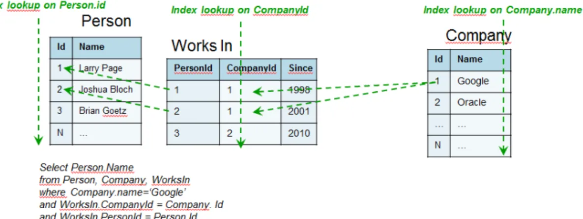
Figure 9: Query execution in graph databases

Relational databases are less adequate to query through relationships. It would mean querying through different tables, following foreign keys and other indexes, and it would considerably increment the performance time. Graph databases traversals are performed by following physical pointers, while foreign keys are logical pointers. [8] The query in the figure, includes the time of each index-scan. The more tables are included in the query, the larger the execution time will become.

Figure 10: Query execution in relational databases

(22)

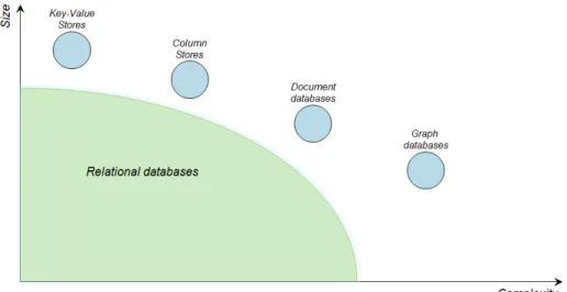
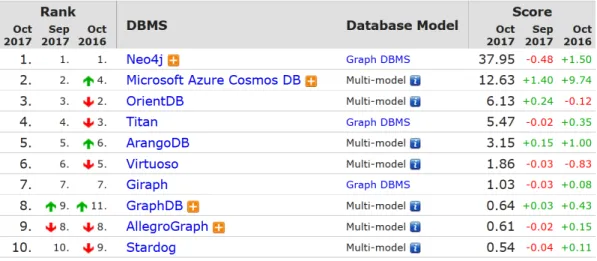
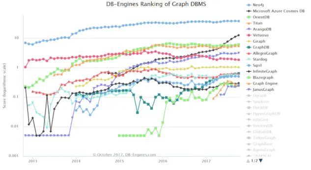
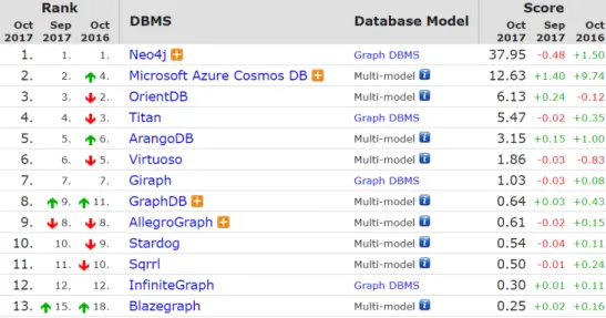
Graph databases ranking Below those lines, the figure shows the DB-Engines Ranking on Graph DBMS.Neo4j leads the ranking, and its score triples the following DBMS,Microsoft Azure Cosmos DB. Neo4j has been leading the Graph databases sector for some years, as we can see in the trend scatter plot. It must be taken into account that the score is displayed in logarithmic scale, therefore the difference in popularity is really significant.

It can also be seen in the trend scatter plot that Microsoft Azure Cosmos DB ap-peared in the graph database landscape in 2014, and since then its rise in popularity has been quite steep. An argument for that is that Microsoft Azure is well integrated in the software marketplace.

Success factor: It has been stated, when comparing the NoSQL DBMS, that graph databases had a limitation in size. Therefore, it is a competitive advantage to work on facilitate the partitioning of a graph. While OrientDB and InfiniteGraph state that they accomplished so,Neo4j seems to be the DBMS that more successfully is improving graph partitioning. [8]

(23)

(24)

3 Neo4j

3.1 Justification of Neo4j

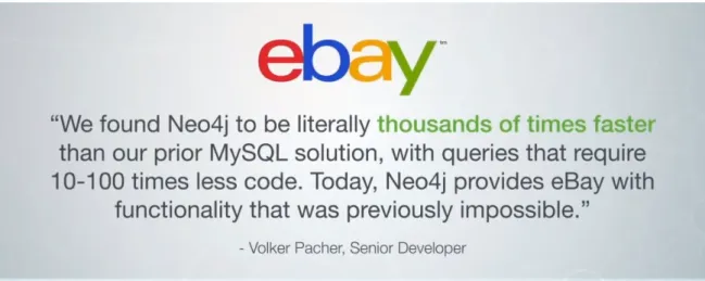
Why Neo4j? By using a graph database like Neo4j which focuses on data rela-tionships; patterns and trends can easily be seen unlike to relational databases. Due to today’s growing business demands and competitive atmosphere, using the right tool is very important and when it comes to widely connected data Neo4j is the best because it is thousands of times faster than traditional databases. Neo4j analyze and traverse of all data in real time and gives the results very fast. Neo4j is widely used by lots of big companies like eBay,Walmart, Cisco, UBS and many more.

(25)

Figure 13: Neo4j As a Leading Graph Database

(26)

Figure 14: Level Of Complexity of Traditional Databases Comparing to Neo4j

Thus, because of the reasons stated above we choose Neo4j as our database.

Figure 15: Ebay’s comment about Neo4j

3.2 Advantages of Neo4j

(27)

• Can represent semi-structured data easily: Data that does not fall into natural structure can be easily represented in a graph database

• Cypher Commands: Cypher commands are human readable and very easy to learn

• Simple and Powerful Data Model: The property graph data model is simple yet still very powerful. The basic building blocks are known to rela-tionships and they can contain data in the form of key value pairs or properties unlike the relational model.

• Join Aspect:There’s no need for complex and costly joins to retrieve con-nected or related data. Instead the graph database uses a natural concept of relationships. Relationships in a graph actually formed paths so querying or traversing a graph involves following those pats and because of that path ori-ented nature of the graph data model, the majority of path based operations are extremely efficient.

• Performance: Traversing a relationship is done in constant time so query performance does not decrease when data grows and Cypher is designed for graphs so it is very simple to write graph traversals based on pattern matching. . Neo4j is only graph database that combines native graph storage, scalable ar-chitecture optimized for speed, and ACID compliance to ensure predictability of relationship-based queries. [10]

• Real-time insights: Neo4j provides results based on real-time data.

• High availability: Neo4j is highly available for large enterprise real-time applications with transactional guarantees.[15]

• Biggest graph community in the world: Neo4j has the largest and most contributor graph community.

(28)

3.3 Properties of Neo4j

Figure 16: General Look at Neo4j

Following are properties of Neo4j;

(29)

• Scalability and reliability: Database can be scaled by increasing the num-ber of reads/writes, and the volume without effecting the query processing speed and data integrity. Neo4j also provides support for replication for data safety and reliability.

• The traversal of the graph: The traversal is the operation of visiting a set of nodes in the graph by moving between nodes connected with relationships. It’s a unique operation to the graph model for data retrieval. Querying the data using a traversal only takes into account the data that’s required, therefore it is not needed to query the entire data set in an expensive operation, like is the case with join operations on relational data. [1]

• Cypher Query Language: Neo4j provides a powerful declarative query lan-guage known as Cypher. It uses ASCII-art for depicting graphs. Cypher is easy to learn and can be used to create and retrieve relations between data without using the complex queries like Joins.[9]

• Built-in web application: Neo4j provides a built-in Neo4j Browser web application. Using this, creating and querying graph data can be done.

• Drivers: Neo4j can work with

1. REST API to work with programming languages such as Java, Spring, Scala etc.

2. Java Script to work with UI MVC frameworks such as Node JS.

3. It supports two kinds of Java API: Cypher API and Native Java API to develop Java applications.

• Indexing: Neo4j supports Indexes by using Apache Lucence.

3.4 Performance In Neo4j

Neo4j provides fast and efficient graph experience and the strongest part of it is; Neo4j can traverse millions of nodes in milliseconds. Also even exponentially increas-ing data size does not effect the performance of Neo4j unlike relational databases.

(30)

Figure 17: Query times for Oracle Exadata vs Neo4j

Figure 18: Tomtom’s Comparison of Neo4j with MySQL

(31)

• In order to avoid costly disk access, making sure of relevant graph data is cached in memory.

• For the non-Neo4j tasks running on the computer a sufficient memory should be reserved.(At least 16G)

• Simple algorithms leads to increased performance.

• All related nodes and edges should be kept in server memory before giving results.

• Traversals should be independent.

• Indexes should be used.

3.5 Cypher Query Language

Cypher is a declarative language for working with graphs and graph data for both reading and writing to the graph and it is very expressive and powerful. Also Cypher defines patterns in the given graph data.

• Cypher is declarative language: This means that we specify the data that we are interested in. We do not specify how to get that data from the database.

• Cypher is very human readable language and it is accessible not just for de-velopers everyone can easily learn and use it.

• Cypher has expressions similar to SQL like WHERE, ORDER BY and simple condition statements like <, =,>. Its difference with sql is; Cypher is designed to represent graph data patterns for example it has MATCH property this property is built on finding and specifying patterns in the data

3.5.1 Structure

(32)

Figure 19: Node Representation

Relationships In Cypher; between the nodes we have lines which represent the relationship between each node. Relationships can also have properties just like nodes which is something that is much different than SQL. Also relationships have directions. Relationship is shown as –> between two nodes.

Figure 20: Relationship Representation

3.5.2 Operations In Cypher

(33)

• DateOfBirth: ’21.05.1994’

• School:’ULB’

With this Cypher code;

CREATE (n:Person {name :’Ozge Koroglu’, country: ’Turkey’, city: ’Istanbul’, DateOfBirth:’21.05.1994’, School:’ULB’}) RE-TURN n

Figure 21: Create Person’s Node

• Name: ’Anna Turu Pi’

• Country: ’Spain’

• City: ’Barcelona’

• DateOfBirth: ’30.07.1995’

• School:’ULB’

(34)

CREATE (n:Person {name :’Anna Turu Pi’, country: ’Spain’, city: ’Barcelona’, DateOfBirth:’30.07.1995’, School:’ULB’}) RETURN n

We created a relationship called "FRIENDS_WITH" with the property "SINCE";

With this Cypher code;

MATCH (a:Person),(b:Person) WHERE a.name = ’Ozge Koroglu’ AND b.name = ’Anna Turu Pi’ CREATE (a)-[r:FRIENDS_WITH {SINCE:"17/09/2017"}]->(b) RETURN r

(a) Result in Console (b) After Creating Relationship

Figure 22: Create Relationship Between Two Nodes

Match: Match finds specified patterns in the data.

(35)

Figure 24: Match Result

Set: This is used to update properties in the nodes and relationships.

With this Cypher Code we changed Esteban Zimányi’s date of birth to ’01.01.1966’

MATCH (n { name: ’Esteban Zimányi’ }) SET n.DateOfBirth = ’01.01.1966’ RETURN n

Delete This operator deletes nodes or relationships in the data.

With this Cypher code we deleted Ozge Koroglu

(36)

Figure 25: Delete Result

3.5.3 Loading Data With Cypher

There are lots of ways to import data in Neo4j but the most common way is upload it as a csv file. Load CSV operator is built into Neo4j and this operator is used for small or medium size datasets up to 10 million records. If we want to upload data that has more than 10 million records than we should use [USING PERIODIC COMMIT[n]] property. If we dont use this property this means that we are processing whole file in one run and creating everything in one transaction

(37)

3.6 Use Cases of Neo4j

Figure 27: Use Cases Of Neo4j

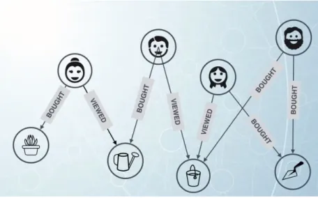
The common use cases are;

(38)

Figure 28: Real Time Recommendations Graph Design

(39)

Fraud Detection: Fraud detection is very important in finance industry. Nowa-days in order not to be detected by bank’s fraud algorithms people use different approaches like open several bank accounts with valid information and do normal transactions without being an outlier. So people open false bank accounts with the same identity token and withdraw all the money in all bank accounts. It is hard to detect that behavior but it is very easy to see that with graph because the pattern of the people opening bank accounts using the same identity token can be easily detected as a pattern in a graph

Graph Based Search: Metadata is available for things like products, articles etc. And being able to model metadata as a graph allows to enhance search meaning users are able to find more relevant things for them. For example LinkedIn; When search is executed we don’t see random or alphabetical sorted results we first see the relevant ones. Lufthansa uses Neo4j for this matter.

Network & IT Operations: If data center is modelled as a graph then depen-dency analysis can easily be applied on network systems to get conclusions like if one virtual machine goes down how many applications will be affected. Hp uses Neo4j to model their network for some large telecommunication providers.

(40)

(41)

4 Neo4j Application

Software For the graph database,Neo4j Community Edition 3.2.5 has been used, and for the relational database, SQL Server 2017.

4.1 Use Case Selected

As proposed in graph database benchmark guidelines [4], the best tests to benchmark a graph database are: traversal (which includes the calculation of the shortest path), graph analysis, connected components, communities, centrality measures, pattern matching and graph anonymisation. It is also commented that among the domains where graph databases prove to be more beneficial are the shortest path graph analysis and real time analysis of traffic networks. In our implementation, we are going to model flight routes, as they have the ideal properties to benchmark a graph database. Airports and airlines are elements where the information lies on the their inter communications.

4.2 Data

The data set selected to perform the benchmark was a data set of flight routes pro-vided by OpenFlights.org [13]. It propro-vided three flat files, airlines.dat, airports.dat, routes.dat.

(42)

4.2.1 Implementing Data

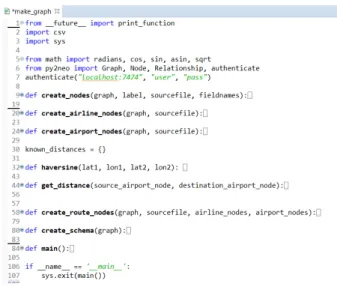
Figure 31: OpenFlights.org

Neo4j: To create the Neo4j database we developed a python code. This code uses py2neo library to access Neo4j database and it reads our data (external source) to create nodes, relationships, properties and indexes

(43)

destination_airportas a name attribute to route node. In the end four types of nodes are Airlines, Airports and Routes, and they have the following communications:

Route → TO → Airport Route → FROM → Airport Route → OF → Airline

Table 2: Graph database schema

We implemented our data to Neo4j with this schema;

(44)

Figure 34: Example of a query in Neo4j

(45)

Figure 35: Relational database diagram

4.2.2 Export data

To export the Neo4j, we chose to use the apoc library. It is needed to authorize Neo4j to run the plugins. For that, this line of code has to be added in neo4j.conf: apoc.export.file.enabled=true.

Export to CSV

apoc.export.csv.query(query,file,config): exports results from the Cypher statement as CSV to the provided file

apoc.export.csv.all(file,config): exports whole database as CSV to the pro-vided file

apoc.export.csv.data(nodes,rels,file,config): exports given nodes and re-lationships as CSV to the provided file

apoc.export.csv.graph(graph,file,config): exports given graph object as CSV to the provided file

(46)

Figure 36: Exporting Neo4j database to CSV file

Figure 37: CSV file containing Neo4j database

Export to cypher script

apoc.export.cypher.all(file,config): exports whole database incl. indexes as Cypher statements to the provided file

apoc.export.cypher.data(nodes,rels,file,config): exports given nodes and relationships incl. indexes as Cypher statements to the provided file

apoc.export.cypher.graph(graph,file,config)exports given graph object incl. indexes as Cypher statements to the provided file

apoc.export.cypher.query(query,file,config): exports nodes and relationships from the Cypher statement incl. indexes as Cypher statements to the provided file apoc.export.cypher.schema(file,config): exports all schema indexes and con-straints to cypher

(47)

Figure 38: Exporting Neo4j database to cypher script

(48)

4.3 Query Examples (Neo4j-SQL)

Figure 40: Algorithms for graph databases

(49)

apoc library).

After that, Neo4j needs to be restarted, and it can be verified that the plugin is working by writing the following command in Neo4j browser:

CALL dbms.procedures() YIELD name, signature, description WHERE name starts with "apoc"

RETURN name, signature, description

4.3.1 Shortest Path

This algorithm is the one that better justifies the existence of graph databases. Its calculation is impossible with SQL. In SQL it is needed to specify the number of layers the route has.

First query example: find the shortest path to go from an airport in Madrid to an airport in Seoul.

MATCH p=shortestpath((src:Airportcity: ’Madrid’)-[r:FROM|TO*..15]-(dest:Airportcity: ’Seoul’)) RETURN p

(50)

Figure 43: Pipeline of the shortest path query

(51)

MATCH p=shortestpath((src:Airport{city: ’Seoul’})-[r:FROM|TO*..15]-(dest:Airport{city: ’Antwerp’})) RETURN p

Figure 45: Shortest path query from Seoul to Antwerp

Paying attention to the relationships, it can be seen that the query doesn’t output a physically possible travelling route from the origin city to the origin city. In the first query, one of the paths ends up in Seoul, but the other has two sources, Madrid and Seoul, and they both end up in Beijing. The second query has three origin airports, one in Antwerp and two in Seoul, and all the routes finish in Geneve.

The purpose of the algorithm is to find the shortest path to connect two nodes, independently of the physical meaning, but real routes can be created with the following modification:

Persistent inferred relationships: For each route going from an airport to an-other, a relationship connecting both airports has been added. This way, the shortest path query can look for only one type of relationship. If the objective is to find phys-ically possible paths between two airports (e.g., not stepping into an airline) it will be assured looking for that inferred relationship that airports are being connected to airports.

RelationshipCONNECTED.This relationship has the property weight, and is pro-portional to the number of routes between two airports. It is being used in the shortest path queries and community detection queries.

(52)

WHERE id(ap1) <> id(ap2)

WITH ap1, ap2, COUNT(*) AS weight CREATE (ap1)-[c:CONNECTED]->(ap2)

SET c.weight = weightIn the figure below the database schema after adding the inferred relationship is displayed:

Figure 46: Neo4j DB schema after adding Connected relationships

Cypher code to delete the relationship:

MATCH (ap1:Airport)-[r:CONNECTED]->(ap2:Airport) DELETE r

Relationship GOINGTO. This relationship saves the route and airline information in its properties. It is being used in the shortest path queries and community detec-tion queries.

Cypher code to create the relationship:

MATCH (ap1:Airport)<-[:FROM]-(r:Route)-[:TO]->(ap2:Airport) WHERE id(ap1) <> id(ap2)

WITH ap1, ap2, r

(53)

displayed:

Figure 47: Neo4j DB schema after adding Goingto relationships

Cypher code to delete the relationship:

MATCH (Airport)-[r:GOINGTO]->(Airport) DELETE r

The first shortest path query is run again now with the inferred relationships:

MATCH p=shortestpath((src:Airport{city: ’Madrid’})-[r:GOINGTO]-(dest:Airport{city: ’Seoul’})) RETURN p

Figure 48: Shortest path between Madrid and Seoul

Now the airports are directly connected to each other. The route node cannot be seen, but its identifier is saved as one of the relationship properties. With the follwoing query it can be verified if the route matches the requisites:

(54)

Figure 49: Shortest path outbound route output

It is verified that the relationship GOINGTO was equivalent to a real outbound route between Madrid and Seoul. The return rout is also verified:

MATCH (r:Route) WHERE id(r)=50205 RETURN r

Figure 50: Shortest path return route output

(55)

(a) From Antwerp to Minneapolis (b) From Antwerp to Mallorca

(c) From Santarem to Eugene (d) From Istanbul to Eugene

(e) From Reykjavik to Eugene

Figure 51: Other shortest path examples

Shortest path in SQL Server: SQL Server has the limitation that it need to be specified the number of layers in the path. An alternative is to use a recursive query, but from our experience, it was not effective.

(56)

Figure 52: SQL Server recursive query output

(57)

(58)

Figure 54: Pipeline of Neo4j query on Antwerp-Istanbul shortest path

4.3.2 Betweenness centrality:

The betweenness centrality of a node in a network is the number of shortest paths between two other members in the network on which a given node appears. Between-ness centality is an important metric because it can be used to identify “brokers of information” in the network or nodes that connect disparate clusters. [6]

(59)

Figure 55: Concept of betweenness centrality

MATCH (ap:Airport)

WITH collect(ap) AS airports

CALL apoc.algo.betweenness([’CONNECTED’], airports, ’OUTGOING’) YIELD node, score

SET node.betweenness = score

RETURN node AS Airport, score ORDER BY score DESC LIMIT 25

Figure 56: Betweenness centrality query result

(60)

intercontinental journeys. It makes sense that they have the highest betwenness centrality.

Query performance: Writing PROFILE before the cypher query, outputs the pipeline of the query execution.

Figure 57: Pipeline of the betweenness centrality query

4.3.3 Closeness centrality:

(61)

Figure 58: Concept of closeness centrality

Query example: output the five airports with a higher closeness centrality: MATCH (ap:Airport)

WITH collect(ap) AS airports

CALL apoc.algo.closeness([’CONNECTED’], airports, ’OUTGOING’) YIELD node, score

RETURN node AS Airport, score ORDER BY score DESC LIMIT 5

Figure 59: Closeness centrality query result

(62)

of Brazil, the Grand Canyon of Colorado...

Figure 60: Location of the airports with highest closeness centrality

(63)

Figure 61: Pipeline of the closeness centrality query

4.3.4 PageRank:

The secret of Google’s success was its search algorithm, PageRank. PageRank works by counting the number and quality of links to a page to determine a rough estimate of how important the website is. The underlying assumption is that more important websites are likely to receive more links from other websites [11]. This algorithm can output the most connected airport or the most powerful airline (the node connected to more routes).

First query: output the most important airports

(64)

(65)

Second query: Output the most popular airlines.

MATCH (node:Airline) WITH collect(node) AS airlines CALL apoc.algo.pageRank(airlines) YIELD node, score RETURN node, score ORDER BY score DESC LIMIT 10

(66)

Figure 65: Pipeline of the airlines pagerank query

As a result we can see that Ryanair is the leading airline, followed by four companies from the USA and three from China.

4.3.5 Community Detection:

There are many algorithms for community detection: triangle counting, strongly connected components, ... This algorithms cluster together the nodes more related with each other. We have chosen an algorithm from the library APOC, and what the code below does, is classify the airport nodes in 40 partitions. The classification is determined on the weight of the connected relationships (the number of routes between each pair of airports).

(67)

to-Graph Databases and Neo4J

Figure 66: Community detection graph

The figure over these lines shows the shape of the graph after the nodes have been classified in partitions. To see which nodes belong to each partition, the partition number must be returned as output:

CALL apoc.algo.community(40,[’Airport’],’partition’, ’CONNECTED’,’OUTGOING’,’weight’,10000)

(68)

(69)

Figure 68: Pipeline of community detection query

(70)

Figure 69: Papua New Guinea partition

The following part of the graph is a bit scattered, but it can be seen that they are all communicated to the central nodes. Hovering over them, we see that they all belong to Canada, and we can suppose that the more separated nodes are regional airports connected to bigger more important airports. That part of the graph is equivalent to seven partitions in the table.

Figure 70: Canada partitions

(71)

Figure 71: Algeria partition

The more centralized part of this subgraph are the airports from Finland. Some of those are connected with a Greenland’s airport, which connects with other Greenland and Iceland airports.

Figure 72: Finland, Greenland, Iceland partitions

(72)

(a) Partition table

(b) Partition graph

Figure 73: Africa partition

(73)

Polynesia, Micronesia and Melanesia. that

(a) Partition table

(b) Geographical location

Figure 75: Australasia partition

4.3.6 Possible queries on SQL

(74)

1. Finding flights between two airports that have no direct route be-tween them: MATCH p=allShortestPaths((ap1:Airport {city:’Antwerp’})-[*]->(ap2:Airport {city:’Istanbul’}))

WITH extract(node in nodes(p)|node.name) as cities, extract(rel in relationships(p)|rel.airline)as airlines RETURN cities,airlines

select distinct A1.Name as [1st Airport]

,airline1.name as [1st Airline],

A2.Name as [2nd Airport], airline2.name as [2nd Airline],

A3.Name [3rd Airport],

airline3.name [3rd Airline], a4.name [4th Airport]

FROM routes r INNER JOIN airports a1

ON r.source_airport_id=a1.ID INNER JOIN airlines airline1 ON airline1.id=r.airline_id INNER JOIN airports a2 ON

r.destination_airport_id=a2.ID INNER JOIN routes r2

on a2.ID=r2.source_airport_id INNER JOIN airlines airline2 on airline2.id=r2.airline_id INNER JOIN airports a3

ON

r2.destination_airport_id=a3.ID INNER JOIN routes r3

(75)

(a) Neo4j Result

(b) SQL Result

Figure 76: Comparison of Queries - first query

As it can be seen from here finding all possible routes between two airports is easy in Neo4j. Besides that Neo4j gives visualization.

(76)

2. Nearest airport to city by distance match(airport1:Airport{city:’Bologna’} )<-[:FROM]- (route:Route) -[:TO]->(airport2:Airport) RETURN airport1, route,airport2

ORDER BY route.distance asc limit 1

Select top 1

A2.name,a2.city,a2.country

,dbo.DistanceKM(a.latitude,a2.latitude, A.longitude, A2.longitude) as

distance from routes r

INNER JOIN airports a

on a.id=r.source_airport_id INNER JOIN airports a2 on

a2.id=r.destination_airport_id WHERE A.city=’Bologna’

order by distance asc

(a) Neo4j Query

(b) SQL query

Figure 77: Comparison of queries - second query

(77)

lat-Graph Databases and Neo4J

3. Most connected airports

MATCH

(airport:Airport)<-[:FROM]-(r:Route) WITH airport, count(r) as

departures MATCH

(r2:Route)-[:TO]->(airport) RETURN airport.name as airport_name, departures , count(r2) as arrivals order by departures+arrivals desc SELECT A.Name,A.City,A.Country,SUM(A.route_count) AS route_count FROM( SELECT a.Name,a.City,a.Country, COUNT(*) as route_count FROM routes R

INNER JOIN airports A ON A.ID=source_airport_id GROUP BY a.Name,a.City,a.Country ) UNION( SELECT a.Name,a.City,a.Country,COUNT(*) as route_count FROM

routes R

INNER JOIN airports A ON A.ID=destination_airport_id GROUP BY

a.Name,a.City,a.Country ))A GROUP BY

(78)

(a) Neo4j Query

(b) SQL query

Figure 78: Comparison of queries - third query

(79)

5 Conclusion

In conclusion, graph databases are necessary for a very concrete data sets: huge amounts of data of high complexity, where entities are very related to one another. That is because, they efficiently query through the relationships among entities, in contrast to relational databases.

Graph databases support algorithms to perform concrete queries that are out of reach to relational databases, for their tabular structure and static schema. Also, the bigger the volume of data, the slower the queries would be in SQL, because they would require to lookup joined tables with a great number of tuples. Graph databases allow to traverse through the graph and reach a high level of depth, without having to read all the data stored.

Neo4j is, by far, the leading technology of graph databases. It analyze and traverse of all data in real time and gives the results very fast. It has great user interface and support. But the greatest feature of it is; even data size grow exponentially, performance of Neo4j does not affected by it.

In our hands on research, we have stored a graph database about flight routes in Neo4j. The same data has been stored in a SQL Server database, in order to proof that some queries are more efficient in Neo4j, and some are even not possible to execute in SQL. We have queried the Shortest Path, PageRank, Betweenness and Closeness Centrality, and Partition for Community Detection.

(80)

Bibliography

[1] Tareq Abedrabbo Dominic Fox Jonas Partner Aleksa Vukotic, Nicki Watt. Neo4j in Action. Manning Publications, 2015.

[2] Stephan C. Carlson. Graph theory. encyclopædia britannica. Available at

https: // www. britannica. com/ topic/ graph-theory, May 2013. Accessed: 2017-11-30.

[3] DB-Engines. Knowledge base of relational and nosql database management systems. Available at https: // db-engines. com/ en/, 2017. Accessed: 2017-10-20.

[4] Martinez-Bazan N. Muntes-Mulero V. Baleta P. Larriba-Pay J.L. Dominguez-Sal, D. A discussion on the design of graph database benchmarks. September 2010.

[5] Stefan Edlich. Nosql archive. Available at http: // nosql-database. org/. Accessed: 2017-11-20.

[6] William Lyon. Analyzing the graph of thrones. Available at http: // www. lyonwj. com/ 2016/ 06/ 26/ graph-of-thrones-neo4j-social-network-analysis/ /, June 2016. Accessed: 2017-12-3.

[7] Mathigon. Graphs and networks. Accessed: 2017-11-30.

[8] Thomas Vial Michel Domenjoud. Graph databases: an overview. OctoTalks, July 2012. Accessed: 2017-11-30.

[9] Neo4j. Intro to cypher.

[10] Neo4j. Top ten reasons for choosing neo4j. Available at https: // neo4j. com/ top-ten-reasons/.

[11] Neo4j. Neo4j graph algorithms. Github, October 2017. Accessed: 2017-12-8.

(81)

[14] Tutorials Point. Graph theory: Introduction. Available at https: // www. tutorialspoint. com/ graph_ theory/ graph_ theory_ introduction. htm. Accessed: 2017-11-30.

[15] Tutorials Point. Neo4j - overview. Available at https: // www. tutorialspoint. com/ neo4j/ neo4j_ overview. htm. Accessed: 2017-11-30.

[16] Bryce Merkl Sasaki. Graph databases for beginners: Acid vs. base explained. Available at https: // neo4j. com/ blog/ acid-vs-base-consistency-models-explained/, September 2015. Ac-cessed: 2017-11-20.

[17] James Serra. Relational databases vs non-relational databases. Big Data and Data Warehousing. James Serra’s Blog, August 2015. Accessed: 2017-11-29.

[18] James Serra. Types of nosql databases. Big Data and Data Warehousing. James Serra’s Blog, April 2015. Accessed: 2017-11-29.

Graph Databases and DBMSs - Free Computer, Programming, Mathematics, Technical Books, Lecture Notes and Tutorials

Université libre de Bruxelles

INFO-H-415

Advanced Databases

Graph Databases and Neo4J

Authors:

Anna

Turu Pi

Ozge

Koroglu

Supervisor:

Esteban

Zimányi

Contents

List of Tables

List of Figures

1

Introduction

2

Background

2.1

State of the art of Databases

2.2

Types of DBMS

2.3

Graph Databases

3

Neo4j

3.1

Justification of Neo4j

3.2

Advantages of Neo4j

3.3

Properties of Neo4j

3.4

Performance In Neo4j

3.5

Cypher Query Language

3.6

Use Cases of Neo4j

4

Neo4j Application

4.1

Use Case Selected

4.2

Data

4.3

Query Examples (Neo4j-SQL)

5

Conclusion

Bibliography

_{Turu Pi}

_Koroglu

_Zimányi