Application of a Genetic Algorithm to Storm Sewer Network Optimization

(1)

Application of a Genetic Algorithm to

Storm Sewer Network Optimization

M.H. Afshar 1

In this paper, a genetic algorithm is developed for the optimal design of storm water networks. The nodal elevations of the sewer network are taken as the decision variables. A steady state simulation code is used to analyze the trial solutions provided by the GA optimizer. The performance of the four selection schemes namely, conventional roulette wheel, roulette wheel selection with linear scaling, roulette wheel selection with ranking and, nally, roulette wheel selection with power law scaling, is studied by applying the model to some benchmark examples in the literature. The conventional roulette wheel selection scheme produced superior results compared to other methods. The results produced by the proposed model are either comparable or superior to existing results in the literature.

INTRODUCTION

Storm water networks are an essential part of the infrastructure of any society. Construction and main-tenance of these large scale networks require a huge amount of investment. Any reduction of total cost in the construction of these networks through proper design would result in considerable savings. Pipes and excavations constitute the main cost of storm water networks, but, reducing the cost of excavations and pipes often creates contradictory objectives in the design of storm water networks. Any reduction in pipe size, under the usual constraints of minimum and maximum velocities, requires an increase in the pipe slope leading to more excavation costs. Reducing the excavation costs, on the other hand, requires milder slopes for the pipe, leading to bigger pipe sizes to carry the design discharge. Any economical design of storm water networks, therefore, requires an optimal trade-o between the pipes and excavation costs, which cannot be achieved by engineering judgments.

An optimal design for storm sewer networks has, therefore, received considerable attention in the past decades. Existing attempts for optimization of storm water networks can be categorized into three groups. Dynamic Programming (DP) methods are the rst and most used method for the optimal design of storm sewer

1. Department of Civil Engineering, Iran University of Science and Technology, Tehran, I.R. Iran.

networks, due to the serial features of these networks. Robinson and Labadie [1], Yen et al. [2], Kulkarni and Khanna [3] and Li et al. [4] employed DP to optimally design storm water networks. Dynamic programming methods, which are theoretically capable of nding the global optimum solution, suer from the so-called curse of dimensionality and, therefore, are not applicable to real-world sewer networks. There have been some attempts, using the linear programming method, to solve the problem of storm water design. Elimam et al. [5] used a combination of Linear Programming (LP) and a heuristic approach to design a large scale storm water network. Heuristic approaches are recently being used for the problem, due to their simplicity and the good results achieved. Miles and Heaney [6] and Afshar and Zamani [7] have used heuristic approaches on spreadsheet templates to get near optimal solutions for the problem.

Evolutionary strategies and, in particular, genetic algorithms have been receiving considerable attention in many areas of the water resources industry. These methods have been successfully used for the optimal design of pipe networks with a xed layout [8-12], the layout optimization of pipe and gas networks [13-16], management of groundwater systems [17-19], cal-ibration of water resources models [20] and reservoir operation problems [21-24]. Genetic algorithms have proved to be very robust as these algorithms do not require the objective function continuity. They can be used for highly nonlinear convex and non-convex

(2)

problems with or without dynamic characteristics. These interesting features of GA explain the wide range of successful applications of the method in dierent areas of water resources engineering.

In this paper, the application of a genetic algo-rithm to the optimal design of storm water networks is addressed. The performance of the method, using dierent selection methods, is studied. The eciency of the method for storm water design is shown by applying the method to two benchmark examples in the literature and presenting the results. The method is shown to produce the best ever achieved solution to the problems considered.

PROBLEM FORMULATION

The problem of storm water network design, in its general form, may be formulated as:

minZ =

n

X

i=1

fi di;Zi;Ci

; (1)

subject to: g1qiQ

i; 8i; (2)

g2ViVmax; 8i; (3)

g3ViVmin; 8i; (4)

g4

y d

i; 8i; (5)

g5SiSmin; 8i; (6)

g6EiEmax; 8i; (7)

g7EiEmin; 8i: (8)

Here:

di pipe diameter in linki,

Zi average excavation depth for linki, Ci unit cost of excavation for linki, qi ow rate in linki,

Q

i design discharge in linki, Vi velocity in linki,

yi ow depth in linki, Si slope of linki, Ei average pipe cover,

Vmin,Vmax minimum and maximum velocity, respectively,

maximum allowable ratio of water to upon pipe diameter,

Emin,Emax minimum and maximum average pipe cover, respectively,

Smin minimum permitted slope (more than zero in general),

n total number of links in the network.

Genetic algorithms are basically designed for uncon-strained optimization problems. Application of GA to constrained optimization problems, such as storm water networks, requires a transform of the underlying constrained problem to an unconstrained optimization problem. Penalty methods are usually used for this purpose, in which the constraints are included in the objective function via a penalty cost term, resulting in the following penalized form of the objective function:

minZp=

n

X

i=1

fi di;Zi;Ci

+f(G); (9)

in whichf is some function of the constraint violation matrixG, with a typical component, gij, representing thejth constraint violation at pipeiandrepresenting the penalty parameter. Dierent forms of function f have been used by dierent researchers. One of the most used forms of function f is the maximum function, which uses the maximum constraint violation in Equation 9 [11,25-27]. In this method, GA could not distinguish between two dierent designs with the same maximum constraint violation but a dierent number of constraint violations. Here, a dierent form of the function is used. For this, rst consider the normalized form of Constraints 2 to 8 as:

g11 qi Q

i 0; 8i; (10)

g2 Vi Vmax

10; 8i; (11)

g31 Vi Vmin

0; 8i; (12)

g4 (y_d)i

10; 8i; (13)

g51 Si Smin

0; 8i; (14)

g6 Ei Emax

10; 8i; (15)

g71 Ei Emin

0; 8i: (16)

The penalized form of the objective function is now dened as:

minZp=

n

X

i=1

fi di;Zi;Ci

+X7

j=1

j

n

X

i=1(

gij)

2

; (17) where gij is the value of the jth constraint violation committed by the corresponding parameter of the ith pipe. Here, all the constraint violations are used for the penalty cost calculation. This method ensures that

(3)

non-proper networks would have more penalty costs and, therefore, leads to a better distribution of the tness function in the search space compared to the conventional method of helping GA to locate useful genes. The use of dierent penalty parameters for each of the constraints oers greater exibility to the GA search engine to locate optimal or near optimal solutions, as will be discussed later.

GA FORMULATION

The following steps are taken in the GA search for optimal design of the storm water networks:

1. Encoding the design variables. The genetic algo-rithm requires that any trial solution of the design problem be represented by a coded string of nite length, similar to the structure of a chromosome of a genetic code. This is usually achieved by dening a selected mapping between the possible values of the design variables and a set of coded sub-strings with a required number of binary bits. For example, a four-bit sub-string can be coded to represent any of the 16 possible values of the design variables. Since nodal cover depth is used as a problem decision variable, a six-bit sub-string is used to represent the 64 possible values obtained by discretization of the range dened by the maximum and minimum allowable nodal cover depth;

2. Generation of an initial population. The GA randomly generates an initial population, of sizeN, of coded strings representing some trial solutions to the storm network design problem;

3. Computation of network cost. Each of the N members of the population is considered in turn and decoded to the corresponding nodal values of the cover depth. The largest possible diameter is then assumed for each pipe of the network, using the resulting pipe slopes, such that the constraint 13 is automatically satised. The cost of each trial solution of the current population is then calculated as the sum of the pipes and excavation costs; 4. Hydraulic analysis of the network. A steady-state

analysis is carried out for each network of the cur-rent population to nd the ow depth and velocity constraint violations. A home-made steady state simulation code is used to analyze the networks; 5. Computation of the total penalized cost. The

penalty cost of the networks in the population is computed if the trial design does not satisfy all the constraints of the problem. The total penalized cost is considered as the sum of the network and penalty cost, as dened in Equation 17;

6. Computation of tness. The tness of a trial design is taken as some function of the total network

cost. Investigators use dierent forms of the tness functions [25,28]. Here, the decit of the total cost from a big number (sum of the maximum and minimum total costs of the networks in the current generation) is used as the tness of each network; 7. Generation of a new population. The GA generates

the members of the new generation by a selection scheme. Dierent selection schemes are suggested in the literature. Here, four dierent selection schemes are considered, as follows:

(a) Conventional Roulette Wheel Scheme (CRWS): In this scheme, the probability of a string i,pi, to be selected for the next generation, is given by:

pi= fi PN

i=1fi

: (18)

This scheme, however, is believed to be the source of the so-called pre-mature convergence, especially in small population genetic searches. Dierent remedies, in the form of scaling or alternative selection operators, are proposed to prevent the dominance of the extraordinary t strings in the early stages of the search [29]; (b) Roulette Wheel Scheme (RWS) with a Power

Law Scaling: In this scheme, a scaling of the form f

0

i = fi is used, where the value of the exponent is designed so thatf

0

max= 5f 0

avg.; (c) Roulette wheel scheme with a linear scaling:

In this scheme, a linear scaling of the form f

0

i = afi+b is used, where the value of the parameters are designed so that the raw and scaled average tness have the same probability of selection andf

0

max= 5f 0

avg;

(d) Roulette wheel scheme with ranking: In this scheme, the population is rst ordered according to the computed tness values and parents are selected with a probability based on their rank in the population [30].

8. The crossover operation. Two o-springs are formed via the partial exchange of bits between two selected parents, using a crossover operator. Crossover occurs with some specied probability of crossover, pc, for each pair of parents selected in the previous step. Here, a one-point cross-over is used in which a point is randomly selected on the strings and, then, the bits before the selected point are exchanged to form two o-springs;

9. Mutation. A bit-wise mutation with some specied probability of mutation,pm, is carried out for each of the strings which have undergone crossover. The bit-wise mutation changes the value of the selected bit to the opposite value (i.e., 0 to 1 or 1 to 0). A one-bit mutation is used in this work;

(4)

Table 1.

Data of the rst benchmark example.

Link Ground Elevation (m) Length (m) Design Discharge (Cm)

Upstream Downstream

1122 152.4 150.876 106.68 0.1132

2233 150.876 148.4876 121.92 0.1982

3342 148.4876 146.304 106.68 0.2548

1232 149.352 147.828 121.92 0.1132

3242 147.828 146.304 131.0761 0.2265 4252 146.304 143.256 167.6796 0.6229 2334 149.352 147.828 147.6375 0.2265

3443 147.828 144.78 137.16 0.3398

4352 144.78 143.256 106.68 0.453

5261 143.256 141.732 152.4 1.2459

3141 147.828 144.78 152.4 0.2548

4151 144.78 143.256 106.68 0.453

5161 143.256 141.732 106.68 0.5663

6171 141.732 138.648 172.212 2.0104

4453 142.6464 141.4272 121.92 0.1132

5362 141.4272 140.208 91.44 0.1699

6271 140.208 138.648 105.2291 0.2548

7181 138.648 137.4648 121.92 2.4635

8191 137.4648 136.5504 152.4 2.5201

9110 136.5504 135.636 186.5376 2.6617

10. Production of successive generations. The three op-erators described above produce a new generation of network trial designs. This procedure is repeated to create successive generations. Typically, a GA will evaluate between 100 and 1000 generations, depending on the problem size. Here, the GA run is allowed for 1000 generations to make sure of the convergence of the dierent selection schemes used.

MODEL APPLICATION

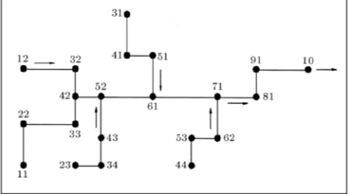
The performance of the proposed GAs is investigated in this section by applying the model to solve two bench-mark problems in the literature. The rst example to be considered is a problem originally designed by Mays and Wenzel [31] and solved by various investigators. The test problem includes 20 links and 21 nodes, as shown in Figure 1. Table 1 presents the characteristic data of the test problem. This problem is constrained to have a maximum velocity of 12 fps (3.6 m/s), a

Figure 1.

Network layout for the rst example.

minimum velocity of 2 fps (0.6 m/s) and a minimum cover of 8 ft (2.4 m). Mays and Wenzel [31] rst used this problem to test the Discrete Dierential Dynamic Programming (DDDP) model they proposed. The DDDP is an iterative technique in which the recursive equation of DP is used to search for an improved trajectory among the discrete states in the

(5)

neighborhood of a trial solution [32]. The problem was later solved by Robinson and Labadie [1] with a dierent version of the dynamic programming model. Miles and Heaney [6] and Afshar and Zamani [7] approached this problem in a spread sheet template. Figure 2 shows the convergence characteristics of the GA methods during the evolution process, while Ta-ble 2 presents and compares the results obtained from the proposed GA methods from the other results in the literature. These results are obtained with a population size of 200, a one-point crossover,pc = 1, and a one-bit mutation per chromosome, pm = 0:5. The best result (202496 units) is obtained with the conventional Roulette Wheel scheme within 145200 evaluations. The good performance of this selection scheme, which is known for premature convergence, can be attributed to the relatively long sub-strings (64 bit) used to represent the allowable variation of the decision variables, resulting in a very large search space. The RWS with linear scaling showed much faster characteristics, yielding the second best result

Figure 2.

Best feasible cost solution of the generations during the evolution process.

Table 2.

Optimal network cost obtained by dierent models for the rst example.

Model

_(units)

Cost

Mays and Wenzel [31] 265,775 Robinson and Labadie [1] 275,218 Miles and Heaney (spreadsheet) [6] 245,874 Afshar and Zamani [7] 221,652 Present model (GA1) 202,496 Present model (GA2) 205,191 Present model (GA3) 217,729 Present model (GA4) 213,000

(205191 units). This result is obtained at the expense of 50000 network evaluations, much less than the number of analyses required by the CRWS. The two other selection schemes showed the same convergence characteristics with similar poorer results. The RWS with ranking converged to a solution with 217729 units of cost within 66000 function evaluations, while the RWS with power law scaling resulted in a solution with 213000 units of cost in about 65000 network simulations. Despite dierent results obtained by the proposed GA method, the resulting solutions are all cheaper than the best ever achieved solution in the literature. This example shows the eciency and eec-tiveness of the genetic algorithm in solving storm water network design problems compared to the existing methods. Details of the optimal solution obtained by the proposed methods are shown in Tables 3 to 6. The best ever result reported in the literature is obtained by Afshar and Zamani [7], using a heuristic approach in a spreadsheet template, which is also shown in Table 7 for comparison.

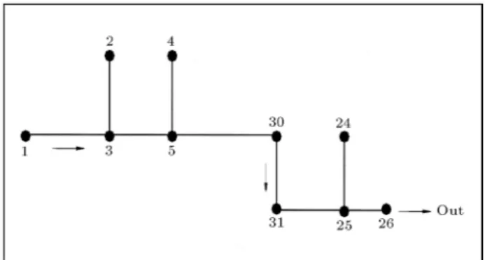
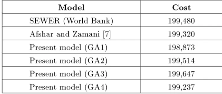
The second example is a network with 9 links and 10 nodes, shown in Figure 3. This network was used by Afshar and Zamani [7] to test their model against the SEWER software developed by the World Bank [33]. Physical and hydrological data of the network are given in Afshar and Zamani [7]. Table 8 shows the cost of the optimal solution obtained with dierent methods, including the proposed GA methods, while the details of the optimal solution obtained by the proposed methods are shown in Tables 9 to 12. Two of the proposed methods resulted in cheaper solutions than previously obtained, while the other two converged to networks with marginally higher costs. The best result is again obtained by the Conventional Roulette Wheel Scheme. The reason GA could not improve the solution as much as the rst example is mostly due to the fact that the second problem is a very easy problem. This is clearly seen by the marginal improvement achieved by the previous model, with respect to the result obtained by SEWER, which is a very basic design code for sewer networks.

(6)

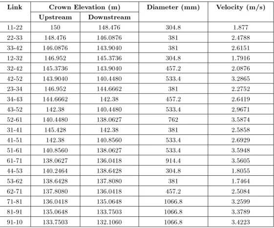
Table 3.

Results obtained from GA1 for the rst example.

Link

Crown Elevation (m)

Diameter (mm)

Velocity (m/s)

Upstream

Downstream

11-22 150 148.476 304.8 1.877

22-33 148.476 146.0876 381 2.4788

33-42 146.0876 143.9040 381 2.6151

12-32 146.952 144.9383 304.8 2.0008

32-42 144.9383 143.9040 457.2 1.8093

42-52 143.9040 140.4933 533.4 3.2659

23-34 146.952 144.5574 381 2.3277

34-43 144.5574 142.38 457.2 2.5864

43-52 142.38 140.4933 533.4 2.939

52-61 140.4933 138.2742 762 3.4784

31-41 145.428 142.38 381 2.5858

41-51 142.38 140.8560 533.4 2.6929

51-61 140.8560 138.2742 533.4 3.4811

61-71 138.2742 136.2480 914.4 3.5651

44-53 140.2464 138.5467 304.8 1.8560

53-62 138.5467 137.7476 381 1.7094

62-71 137.7476 136.2480 457.2 2.3525

71-81 136.2480 135.0648 1066.8 3.5509

81-91 135.0648 133.8504 1066.8 3.2538

91-10 133.8504 132.2087 1066.8 3.4195

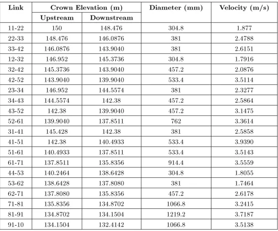
Table 4.

Link

Crown Elevation (m)

Diameter (mm)

Velocity (m/s)

Upstream

Downstream

11-22 150 148.476 304.8 1.877

22-33 148.476 146.0876 381 2.4788

33-42 146.0876 143.9040 381 2.6151

12-32 146.952 145.3736 304.8 1.7916

32-42 145.3736 143.9040 457.2 2.0876

42-52 143.9040 140.4480 533.4 3.2865

23-34 146.952 144.6662 381 2.2752

34-43 144.6662 142.38 457.2 2.6419

43-52 142.38 140.4480 533.4 2.9671

52-61 140.4480 138.0627 762 3.5874

31-41 145.428 142.38 381 2.5858

41-51 142.38 140.8560 533.4 2.6929

51-61 140.8560 138.0627 533.4 3.5948

61-71 138.0627 136.0418 914.4 3.5605

44-53 140.2464 138.6428 304.8 1.8055

53-62 138.6428 137.8080 381 1.7464

62-71 137.8080 136.0418 457.2 2.5084

71-81 136.0418 135.0648 1066.8 3.2599

81-91 135.0648 133.7503 1066.8 3.3789

(7)

Table 5.

Link

Crown Elevation (m)

Diameter (mm)

Velocity (m/s)

Upstream

Downstream

11-22 150 148.476 304.8 1.877

22-33 148.476 146.0876 381 2.4788

33-42 146.0876 143.5942 381 2.7792

12-32 146.952 145.3736 304.8 1.7916

32-42 145.3736 143.5942 457.2 2.2500

42-52 143.5942 139.4053 533.4 3.5822

23-34 146.952 144.5574 381 2.3277

34-43 144.5574 142.38 457.2 2.5864

43-52 142.38 139.4053 457.2 3.4301

52-61 139.4053 137.6396 762 3.1316

31-41 145.428 142.38 381 2.5858

41-51 142.38 140.3573 533.4 3.0219

51-61 140.3573 137.6396 533.4 3.5550

61-71 137.6396 136.2480 1066.8 3.1798

44-53 140.2464 138.6428 304.8 1.8055

53-62 138.6428 137.8080 381 1.7464

62-71 137.8080 136.2480 457.2 2.3895

71-81 136.2480 135.0648 1066.8 3.5509

81-91 135.0648 133.8504 1066.8 3.2538

91-10 133.8504 132.2087 1066.8 3.4195

Table 6.

Link

Crown Elevation (m)

Diameter (mm)

Velocity (m/s)

Upstream

Downstream

11-22 150 148.476 304.8 1.877

22-33 148.476 146.0876 381 2.4788

33-42 146.0876 143.9040 381 2.6151

12-32 146.952 145.3736 304.8 1.7916

32-42 145.3736 143.9040 457.2 2.0876

42-52 143.9040 139.9040 533.4 3.5114

23-34 146.952 144.5574 381 2.3277

34-43 144.5574 142.38 457.2 2.5864

43-52 142.38 139.9040 457.2 3.1475

52-61 139.9040 137.8511 762 3.3614

31-41 145.428 142.38 381 2.5858

41-51 142.38 140.4933 533.4 3.9390

51-61 140.4933 137.8511 533.4 3.5143

61-71 137.8511 135.8356 914.4 3.5559

44-53 140.2464 138.6428 304.8 1.8055

53-62 138.6428 137.8080 381 1.7464

62-71 137.8080 135.8356 457.2 2.6178

71-81 135.8356 134.8702 1066.8 3.2415

81-91 134.8702 134.1504 1219.2 3.7187

(8)

Table 7.

Results reported by Afshar and Zamani [7].

Link

Crown Elevation (m)

Diameter (mm)

Velocity (m/s)

Upstream

Downstream

11-22 150 148.36 304.8 1.66

22-33 148.38 146 381 2.25

33-42 145.84 143.76 381 2.25

12-32 146.91 145.35 304.8 1.57

32-42 145.27 143.9 457.2 1.86

42-52 143.60 140.35 533.4 2.8

23-34 146.95 145.4 457.2 1.86

34-43 145.29 142.38 457.2 2.64

43-52 142.16 140.85 533.4 2.23

52-61 140.10 138.8 914.4 2.66

31-41 145.4 142.38 381 2.56

41-51 142.22 140.8 533.4 2.32

51-61 140.63 138.9 533.4 2.26

61-71 138.58 136.03 914.4 3.49

44-53 140.24 138.7 304.8 1.56

53-62 138.62 137.75 381 1.57

62-71 137.67 136.28 457.2 2.09

71-81 135.65 135.06 1219.2 2.42

81-91 134.87 134.15 1219.2 2.4

91-10 133.97 131.8 1066.8 3.43

Table 8.

Cost of the optimal network obtained for the second example.

Model

Cost

SEWER (World Bank) 199,480 Afshar and Zamani [7] 199,320 Present model (GA1) 198,873 Present model (GA2) 199,514 Present model (GA3) 199,647 Present model (GA4) 199,237

Table 9.

Results obtained from GA1 for the second example.

Link

Crown Elevation (m)

Diameter (mm)

Velocity (m/s)

Upstream

Downstream

1-3 1394.6 1386.7667 150 2.0573

2-3 1393.9 1387.1000 250 2.0532

3-5 1387.1000 1380.0667 300 2.4834

4-5 1385.5 1380.0667 300 2.3450

5-30 1380.0667 1378.1190 450 2.489

30-31 1378.1190 1377.5000 450 2.2016

31-25 1377.5000 1374.4762 450 2.4347

24-25 1376. 6143 1374.4762 150 2.436

(9)

Table 10.

Link

Crown Elevation (m)

Diameter (mm)

Velocity (m/s)

Upstream

Downstream

1-3 1394.6 1386.3381 150 2.1321

2-3 1393.9 1386.3381 250 2.1406

3-5 1386.3381 1379.4476 300 2.4627

4-5 1385.5 1379.4476 300 2.4497

5-30 1379.4476 1377.5476 450 2.4639

30-31 1377.5476 1376.7381 450 2.4835

31-25 1376.7381 1374.3810 450 2.1719

24-25 1376. 5190 1374.3810 150 2.4936

25-26 1374.3810 1371.0 500 2.4696

Table 11.

Link

Crown Elevation (m)

Diameter (mm)

Velocity (m/s)

Upstream

Downstream

1-3 1394.6 1386.3381 150 2.1321

2-3 1393.9 1386.3381 250 2.1406

3-5 1386.3381 1379. 2571 300 2.4902

4-5 1385.5 1379. 2571 300 2.4802

5-30 1379. 2571 1377. 3571 450 2.4639

30-31 1377. 3571 1376.7381 450 2.2016

31-25 1376.7381 1374.3810 450 2.1719

24-25 1376. 1381 1374.3810 150 2.2778

25-26 1374.3810 1371.0 500 2.4696

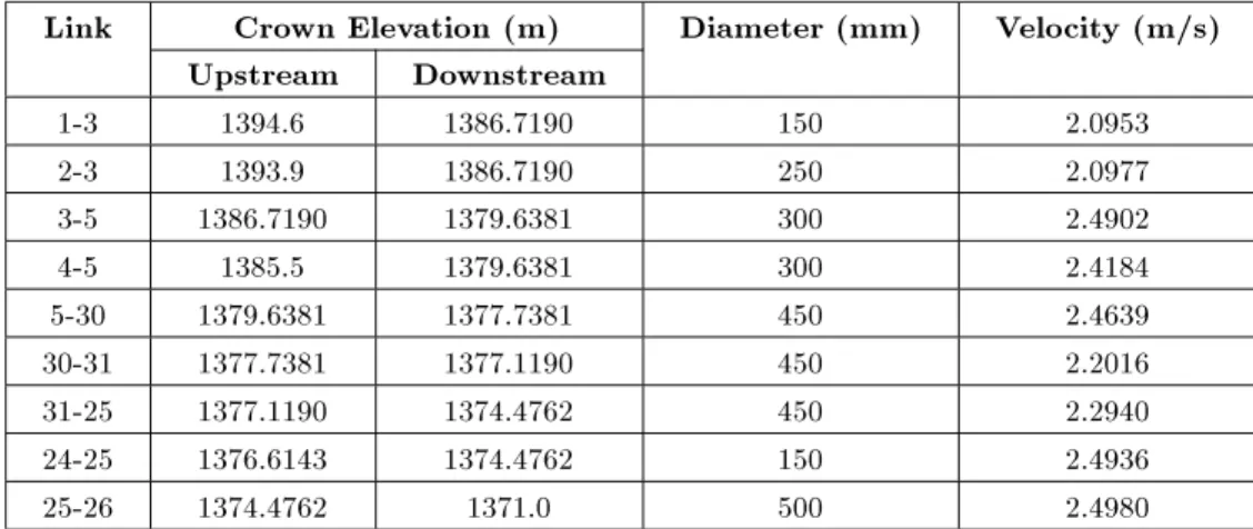
Table 12.

Link

Crown Elevation (m)

Diameter (mm)

Velocity (m/s)

Upstream

Downstream

1-3 1394.6 1386.7190 150 2.0953

2-3 1393.9 1386.7190 250 2.0977

3-5 1386.7190 1379.6381 300 2.4902

4-5 1385.5 1379.6381 300 2.4184

5-30 1379.6381 1377.7381 450 2.4639

30-31 1377.7381 1377.1190 450 2.2016

31-25 1377.1190 1374.4762 450 2.2940

24-25 1376.6143 1374.4762 150 2.4936

25-26 1374.4762 1371.0 500 2.4980

CONCLUDING REMARKS

A genetic algorithm is proposed for the optimal design of storm water networks. The performance of four dierent selection schemes is tested by solving two benchmark problems in the literature. The Conven-tional Roulette Wheel Selection Scheme proved to be

the most ecient method regarding the optimality of the solution. The Roulette Wheel Selection Scheme with linear scaling, however, showed superior conver-gence characteristics, yielding a near optimal solution compared to the conventional scheme. All GA methods resulted in cheaper solutions, compared to the previous results obtained for the larger rst example. The GA

(10)

method failed to considerably improve previous results for the smaller network, mostly due to the simplicity of the considered network. This shows that genetic algorithms might be most ecient for solving large scale real-world problems where other methods often fail.

REFERENCES

1. Robinson, D.K. and Labadie, J.W. \Optimal design of urban storm water drainage system",Int. Symposium on Urban Hydrology, Hydraulics, and Sediment Con-trol, University of Kentucky, Lexington, KY, USA, pp 145-156 (1981).

2. Yen, B.C., Cheng, S.T., Jun, B.H., Voohees, M.L. and Wenzel, H.G. \Illinois least cost sewer system design model, user's guide", Dept. of Civil Engineering, University of Texas at Austin, USA (1984).

3. Kulkarin, V.S. and Khanna, P. \Pumped wastewater collection systems optimization",J. of Environmental Engineering, ASCE,

111

(5), pp 589-601 (1985). 4. Li, G., and Matthew, R.G.S. \New approach for

optimization of urban drainage systems", J. of En-vironmental Engineering, ASCE,

116

(5), pp 927-944 (1990).

5. Elimam, A.A., Charalambous, C. and Ghobrial, F.H. \Optimum design of large sewer networks", J. of Environmental Engineering, ASCE,

115

(6), pp 1171-1189 (1989).

6. Miles, S.W. and Heaney, J.P. \Better than optimal method for designing drainage systems", J. of Wat. Resour. Plng. and Mgmt., ASCE,

114

(5), pp 477-499 (1988).

7. Afshar, A. and Zamani, H. \An improved storm water network design model in spreadsheet template",Int. J. of Engrg. and Science, Iran University of Science and Technology,

13

(4), pp 135-148 (2002).

8. Goldberg, D.E. and Kuo, C.H. \Genetic algorithms in pipeline optimization", J. of Computing in Civil Engineering, ASCE,

1

(2), pp 128-141 (1987).

9. Murphy, L.J., Simpson, A.R. and Dandy, G.C. \Design of a network using genetic algorithms",Water,

20

, pp 40-42 (1993).

10. Simpson, A.R., Dandy, G.C. and Murphy, L.J. \Ge-netic algorithms compared to other techniques for pipe optimization", J. of Wat. Resour. Plng. and Mgmt., ASCE,

120

(4), pp 423- 443 (1994).

11. Savic, D.A. and Walters, G.A. \Genetic algorithms for least-cost design of water distribution networks",J. of Wat. Resour. Plng and Mgmt., ASCE,

123

(2), pp 67-77 (1997).

12. Wu, Z.Y. and Simpson, A.R. \Competent genetic evo-lutionary optimization of water distribution system",

J. of Comput. Civil Eng.,

15

(2), pp 89-101 (2001). 13. Davidson, J.W. and Goulter, I.C. \Evolution program

for the design of rectilinear branched distribution sys-tems", J. of Computing in Civil Engineering, ASCE,

9

(2), pp 112-121 (1995).

14. Walters, G.A. and Lohbeck, T.K., \Optimal layout of tree networks using genetic algorithms", Engineering Optimization,

22

, pp 27-48 (1993).

15. Walters, G.A. and Smith, D.K. \Evolutionary design algorithm for optimal layout of tree networks", Engi-neering Optimization,

24

, pp 261-268 (1995).

16. Davidson, J.W. \Evolution program for layout ge-ometry of rectilinear looped networks", Journal of Computing in Civil Engineering, ASCE,

13

(4), pp 246-253 (1999).

17. McKinney, D.C. and Lin, M.D. \Genetic algorithm solution of groundwater management models",Water Resour. Res.,

30

(6), pp 1897-1906 (1994).

18. Ritzel, B.J., Ehearrt, J.W. and Ranjithan, S. \Us-ing genetic algorithms to solve a multiple objective groundwater pollution problem",Water Resour. Res.,

30

(5), pp 1589-1603 (1994).

19. Cieniawski, S.E., Eheart, J.W. and Ranjithan, S. \Using genetic algorithms to solve a multi-objective groundwater monitoring problem", Water Resour. Res.,

31

(2), pp 399-409 (1995).

20. Wan, B. and James, W. \SWMM calibration using genetic algorithms", Chapter 7 in Best Modelling Practice for Urban Water Systems, Monograph 10 published by CHI, Guelph, Ontario, Canada, ISBN 0-9683681-6-6 CHI catalog Number. R208 (2002). 21. Esat, V. and Hall, M.J. \Water resources system

optimization using genetic algorithms." Hydroinfor-matics 94, Proc., 1st. Int. Conf. on HydroinforHydroinfor-matics, Balkema, Rotterdam, The Netherlands, pp 225-231 (1994).

22. Fahmy, H.S., King, J.P., Wentzel, M.W. and Seton, J.A. \Economic optimization of river management using genetic algorithms",Int. Summer Meeting, Am. Soc. Agric. Engrs. (943034), St. Joseph, Mich, USA (1994).

23. Oliveira, R. and Loucks, D.P. \Operating rules for multi-reservoir systems", Water Resour. Res.,

33

(4), pp 839-852 (1997).

24. Wardlaw, R. and Sharif, M. \Evaluation of genetic algorithms for optimal reservoir system operation",J. of Wat. Resour. Plng. and Mgmt., ASCE,

125

(1), pp 25-33 (1999).

25. Dandy, G.C., Simpson, A.R. and Murphy, L.J. \An improved genetic algorithm for pipe network optimiza-tion",Wat. Resour. Res.,

32

(2), pp 449-458 (1996). 26. Abebe, A.J. and Solomatine, D.P. \Application of

global optimization to the design of pipe networks",

3rd Int. Conf. on Hydroinformatics, Copenhagen, pp 989-996, Balkema, Netherlands (1999).

27. Boulos, P.F., Wu, Z.Y., Orr, C.H. and Ro, J.J. \Least-cost design and rehabilitation of water distribution systems using genetic algorithms", Proceedings of the AWWA IMTech Conference, April 16-19, Seattle, WA, USA (2000).

(11)

28. Gen, M. and Cheng, R., Genetic Algorithms and Engineering Design, John Wiley & Sons, NY, USA (1997).

29. Goldberg, D.E., Genetic Algorithms in Search, Opti-mization & Machine Learning, Addison-Wesley pub-lishing Co, Reading, UK (1989).

30. Grefenstette, J.J. and Backer, J.E. \How genetic algorithms work: A critical look at implicit paral-lelism", Proc., 3rd Int. Conf. of Genetic Algorithms, J.D. Schaer, Ed., Morgan Kaufmann Publishers, San Mateo, Calif., USA pp 20-27 (1989).

31. Mays, L.W. and Wenzel, H.G. \Optimal design of multi-level branching sewer systems",Water Resour. Res.,

12

(5), pp 913-917 (1976).

32. Heidari, M., Chow, V.T., Kokotovic, P.V., Mered-ith, D.D. \Discrete dierential dynamic programming approach to water resources systems optimization",

Water Resou. Res.,

7

(2), pp 273-282 (1971).

33. World Bank, SEWER design package, New York, USA (1991).