1
Changes in significant and maximum wave heights in the Norwegian Sea 2
3
Xiangbo Feng1,2*, M. N. Tsimplis1, M. J. Yelland1and G. D. Quartly3
4 5
1 National Oceanography Centre, Southampton, UK
6
2 School of Ocean and Earth Science, University of Southampton, UK
7
3 Plymouth Marine Laboratory, Plymouth, UK
8 9 10
*Corresponding author address: National Oceanography Centre, Southampton,
11
European Way, Southampton SO14 3ZH, UK 12
Email: xiangbo.feng@soton.ac.uk 13
14 �����������
Abstract
15
This paper analyses 10 years of in-‐situ measurements of significant wave height 16
(Hs) and maximum wave height (Hmax) from the ocean weather ship Polarfrontin 17
the Norwegian Sea. The 30-‐minute ship-‐borne wave recorder measurements of 18
Hmax and Hsare shown to be consistent with theoretical wave distributions. The 19
linear regression between Hmax and Hs has a slope of 1.53. Neither Hs nor Hmax 20
show a significant trend in the period 2000-‐2009. These data are combined with 21
earlier observations. The long-‐term trend over the period 1980-‐2009 in annualHs 22
is 2.72�0.88 cm/year. Mean Hs and Hmax are both correlated with the North 23
Atlantic Oscillation (NAO) index during winter. The correlation with the NAO 24
index is highest for the more frequently encountered (75th percentile) wave
25
heights. The wave field variability associated with the NAO index is reconstructed 26
using a 500-‐year NAO index record.HsandHmaxare found to vary by up to 1.42 m 27
and 3.10 m respectively over the 500-‐year period. Trends in all 30-‐year segments 28
of the reconstructed wave field are lower than the trend in the observations 29
during 1980-‐2009. The NAO index does not change significantly in 21st century
30
projections from CMIP5 climate models under scenario RCP85, and thus no NAO-‐ 31
related changes are expected in the mean and extreme wave fields of the 32
Norwegian Sea. 33
Keywords
: significant wave height; maximum wave height; Ship-‐Borne Wave 34Recorder; NAO; Norwegian Sea 35
1. Introduction
36
Large ocean waves pose significant risks to ships and offshore structures. The 37
development of offshore installations for oil and gas extraction and for renewable 38
energy exploitation requires knowledge of the wave fields and any potential 39
changes in them. Most information presently available for wave fields is 40
presented in terms of the significant wave height (Hs), which is defined as the 41
average height of the highest one-‐third of the waves or, alternatively, as four 42
times the square root of the zeroth moment of the wave spectrum (Sverdrup and 43
Munk, 1947; Phillips, 1977). Knowledge of the maximum peak-‐to-‐trough wave 44
height (Hmax) is not usually available although these largest waves have the 45
greatest impact on ships and offshore structures. 46
The OWS Polarfront, the last weather ship in the world, made measurements ofHs 47
for 30 years using a Ship-‐Borne Wave Recorder (SBWR). The ship was located at 48
Ocean Wea���������������������������������� ���, see Figure 1) in the Norwegian 49
Sea. Waves observed using SBWRs at other stations have been systematically 50
validated against wave buoys in terms ofHsand spectrum byGraham et al(1978), 51
Crisp (1987) and Pitt (1991). However in this study we also use Hmax from the 52
SBWR which has not previously been validated against other wave measuring 53
devices. By analysing the statistical relationship between HsandHmaxas measured 54
by the SBWR and comparing it with the known theoretical and empirical 55
relationships we indirectly provide confidence for the validity of the Hmax 56
measurements. 57
The wind field over the North Atlantic is related to the North Atlantic Oscillation 58
(NAO), a major large-‐scale atmospheric pattern in this region (Hurrell, 1995; 59
Hurrell and Van Loon, 1997; Osborn et al., 1999). The status of the NAO is 60
represented by the NAO index, determined from the non-‐dimensional sea level 61
pressure difference between the Icelandic Low and the Azores High. The NAO is 62
particularly important in winter, and Bacon and Carter (1993) were the first to 63
note the link between this large weather pattern and the wave climate over the 64
North Atlantic. An increase inHsin the North Atlantic over the second half of the 65
20th century was found be associated with the NAO index variability (Bacon and
66
Carter, 1993;Kushnir et al., 1997;Wang and Swail,2001, 2002; Woolf et al.,2002; 67
Wolf and Woolf, 2006). In addition, linear regressions between the inter-‐annualHs 68
anomalies and the NAO index have been established for various methods of wave 69
height estimation (e.g. in-‐situ measurements, visual observations, satellite 70
altimetry and numerical models) (Bacon and Carter, 1993;Gulev and Hasse, 1999; 71
Woolf et al., 2002; Wang et al., 2004; Tsimplis et al., 2005). Hindcasts from 72
numerical models suggest that the influence of the NAO extends to the largest 1% 73
ofHsin the North Atlantic during winter (Wang and Swail,2001, 2002). Izaguirre 74
et al.(2010) using satellite Hsdata also indicated that along the Atlantic coast of 75
the Iberian peninsula the extreme wave climate is significantly associated with 76
the NAO. 77
Thus there is a well-‐established relationship between Hs and the NAO index 78
during winter. The two terms, Hmax and Hs are both characteristics of the wave 79
field and both increase with increasing winds or increasing durations of a 80
consistent wind.Hsis governed by the mean conditions; howeverHmaxis not fully 81
determined by the mean conditions but is also affected by local conditions as well 82
as randomness. Hmax is the pertinent parameter for describing risks associated 83
with operation of ships or offshore structures, hence it is important that we 84
analyze both these measures of the wave field in a consistent manner to show 85
how they differ. 86
In this paper, we investigate Hs and Hmax using 10 years of 30-‐minute surface 87
elevation records from the SBWR at OWS Mike in the Norwegian Sea. First we 88
assess the validity of the dataset by comparing the observational distributions of 89
Hmax and theHmax/Hs ratio with the corresponding theoretical distributions. We 90
establish that the HsandHmax data obtained from the SBWR behave as expected 91
on the basis of theoretical distributions that have been tested against other wave 92
measuring systems. Thus this provides evidence that the Hmaxfrom the SBWR are 93
reliable. We then explore the relationships of the inter-‐annual changes inHsand 94
Hmaxwith the NAO index. We also use a 500-‐year NAO index record to reconstruct 95
the range of values thatHsandHmaxmay have had over the same period. 96
The paper is structured as follows. The data processing and methodology are 97
described in Section 2, along with the statistical definitions to be used. In this 98
section a comparison of the expected distributions for Hs and Hmax with the 99
observed distributions is made. In Section 3, the temporal variability of Hs and 100
Hmax are described, and is correlated with the winter NAO index. The results are 101
discussed in Section 4 where also the natural variability of the wave field over the 102
past 5 centuries is estimated from a reconstruction of the NAO index. Outputs 103
from the most recent CMIP5 models are also used to infer changes in the NAO 104
index under climate change scenarios, and hence assess the likely overall change 105
of the wave fields in the 21stcentury. Our conclusions are given in Section 5.
106 107
2. Data and methodology
108
2.1. Ship-‐Borne Wave Recorder (SBWR) data
109
������������������������������������������������������������������������������
110
occupied by weather ships for more than 60 years until the ship Polarfront was 111
withdrawn at the end of 2009. Sea surface elevation has been measured by a Ship-‐ 112
Borne Wave Recorder (SBWR) and wave height data from this system are 113
available from 1980 to the end of 2009. 114
The SBWR was developed by the UK National Institute of Oceanography (later to 115
become part of the National Oceanography Centre) in the 1950s and is considered 116
a very reliable system (Graham et al., 1978; Holliday, et al., 2006). The principles 117
of operation of the SBWR are described in detail byTucker and Pitt(2001). Using 118
13 years of data from three different weather ships stationed on the UK 119
continental shelf, Graham et al (1978) demonstrated that Hs values from the 120
SBWR were 8% larger than those from WaveRider buoys on average, with closer 121
agreement at larger wave heights.Crisp (1987) examined the wave spectra, and 122
found that the frequency response of the SBWR differed from that of the 123
WaveRider. Pitt(1991) developed an empirical frequency-‐response correction for 124
the SBWR and this reduced the overestimation of Hs to 5%. A short, 30-‐hour 125
comparison between observations obtained on Polarfront and those from a 126
WaveRider buoy also found good agreement, but in this case the SBWR 127
underestimated the Hsslightly, by 0.4 m on average (Clayson, 1997). HenceHs data 128
from the SBWR are well validated. 129
From 1980 until the end of 1999, only the integrated wave parameters (e.g.Hsand 130
average period) were recorded by the SBWR system on Polarfront: these have 131
been analysed briefly elsewhere (Yelland et al., 2009). However, for the last 10 132
years of operation (2000-‐2009, the period investigated in this paper) the SBWR 133
system also recorded the sea surface elevation every 0.59 s for the 30-‐minute 134
sampling periods, with sampling occurring once every 90 minutes before the 135
250th day of 2004, and once every 45 minutes thereafter. Tests made by sub-‐
136
sampling data in the latter period to replicate the earlier 90-‐minute observational 137
interval showed that the change in the observation interval in 2004 has no impact 138
on the results discussed in the rest of this paper. 139
Polarfrontwas allowed to drift freely within a 32 km radius around OWS Mike. 140
Once outside this radius the ship returned on station with a speed of up to 5 m/s. 141
Some of the 30-‐minute records obtained while the ship was steaming were found 142
to contain unrealistically large elevations. All spurious elevations when the ship 143
was steaming were excluded from the analysis during quality control. The wave 144
data during the periods when the Polarfront returned to port, 3 days out of every 145
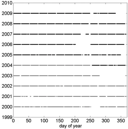
28-‐day period, were omitted because the ship was not on station. A summary of 146
the data record, after application of quality control, is provided in Figure 2. 147
The height of an individual wave is defined as the vertical distance between a 148
wave trough and the following wave crest. There are 17,389,559 individual waves 149
in a total of 71,210 thirty-‐minute wave records obtained over 2,915 days between 150
2000 and 2009. For each 30-‐minute record, the highest individual wave is 151
identified as Hmax, and Hs is calculated from four times the square root of the 152
zeroth-‐order moment of the wave frequency spectrum. 153
2.2. Statistical distribution of waves
155
This section briefly describes statistical distributions in theories for wave fields 156
which have been verified against data obtained from bottom-‐mounted sensors, 157
buoys and altimeters (Bretschneider, 1959; Dobson et al., 1987; Sterl et al., 1998; 158
Tucker and Pitt, 2001; Stansell, 2004; Vandever et al., 2008; Casas-‐Prat and 159
Holthuijsen, 2010). These statistical distributions are then used to validate the 160
SBWR measurements of Hmax and other extreme wave conditions from the 161
Polarfront. This is needed because, unlike Hs, Hmax data from the SWBR have not 162
been validated previously. 163
Individual wave heights with a narrow-‐band spectrum are found to follow a 164
Rayleigh distribution in the deep sea (Longuet-‐Higgins, 1952). Within this 165
narrow-‐band spectrum of wave heights, the average height of the highest one-‐ 166
third of the waves over an observational period, H1/3, is practically equal to the 167
significant wave height,Hs, that can be derived from the spectrum (Phillips,1977). 168
The ratio of observed maximum wave height Hmax to Hs can be theoretically 169
presented as a function of N, the number of individual crest-‐to-‐trough waves 170
measured during an observational period (Sarpkaya and Isaacson, 1981): 171
H��� Hs �
��N
���� (1)
Thus, if NandHsare known, the probable maximum wave height
H
���� in a given 172period can be calculated using Eq. (1). 173
However, Eq. (1) has been found to overestimate the largest individual wave 174
heights when compared to observations (Forristall, 1978;Tayfun, 1981;Krogstad, 175
1985; Massel, 1996; Nerzic and Prevosto, 1997; Mori et al., 2002; Casas-‐Prat and 176
Holthuijsen, 2010). Some of the discrepancy has been attributed to the effect of 177
the spectral bandwidth, i.e. the gathering of wave components around the peak 178
energy component (Tayfun, 1981; Ochi, 1998; Vandever etal., 2008). When the 179
spectral bandwidth increases, Hs is overestimated compared with H1/3 (Tayfun, 180
1981; Ochi, 1998; Vandever et al., 2008). This, in turn, will result in an 181
overestimation of
H
���� estimated from Eq. (1). The nonlinearity of wave-‐wave 182interaction has also been found to affect the crest height and trough depth 183
distributions, but not the peak-‐to-‐trough wave height distributions in 184
observations [Tayfun, 1983; Casas-‐Prat and Holthuijsen, 2010]. More recent 185
laboratory and theoretical work has suggested that nonlinearity may also have 186
some effect on wave height distribution, depending upon the state of wave 187
development (Sluryaev and Sergeeva, 2012;Ying and Kaplan, 2012). 188
Forristall(1978) and Gemmrich and Garrett (2011) have shown that the Weibull 189
distribution provides a better estimate of the observed largest wave heights, i.e. 190
those with the lowest probability of occurrence.Forristall(1978) suggested that a 191
correction to the Hmax derived from the Rayleigh distribution based on the 192
number of waves in the observational record improves the agreement with the 193
Hmax estimated from the Weibull distribution. This is supported by the results of 194
Casas-‐Prat and Holthuijsen(2010). Thus the corrected Rayleigh distribution is an 195
adequate approximation of the wave field parameters as measured by various 196
wave-‐measuring platforms. In the absence of direct evaluation of Hmax from the 197
SBWR against another wave measuring platform we examine the measured 198
statistics to enquire whether the same behaviour of extremes is observed. 199
Comparison with SBWR measurements
200
The average ratio of the theoretically estimated from Eq. (1) to the observed 201
Hmax from the 30-‐minute records is 1.09, indicating that in SBWR measurements 202
the Rayleigh distribution overestimates the maximum wave height by 9%. This 203
confirms the overestimation of Hmax using the Rayleigh distribution in other 204
platforms (Forristall, 1978; Tayfun, 1981; Krogstad, 1985; Massel, 1996; Nerzic 205
and Prevosto, 1997;Mori et al., 2002;Casas-‐Prat and Holthuijsen, 2010). In Figure 206
3 the ratio of
H
���� /Hmax is plotted against N, the number of waves in the 30-‐ 207minute measurement periods. The mean ratio (the black line) increases with 208
increasing N, but individual values over 30-‐minute periods show significant 209
variation, as indicated by the large error bars. 210
The ratio suggests that forHs>10 m the Rayleigh distribution overestimates Hmax 211
by 4% on average and for the annual highest sea states, as listed in Table 1,Hmaxis 212
overestimated by 5%. The discrepancy between
H
���� and Hmax is mainly due to 213the overestimation ofHmax/Hs(that will be discussed later) and may also be due to 214
the effect of spectral bandwidth on the estimate ofHs. 215
Forristall(1978) suggests an empirical correction coefficient of between 0.90 and 216
0.96 (depending on N) to bring the Rayleigh distribution estimates of
H
���� into 217better agreement with those from a Weibull distribution. The average ratio of 218
corrected
H
���� to observedHmax is 0.99. The ratio against Nis shown in Figure 3 219by the grey line. The trend with Nand the noise in the individual ratios (see error 220
bars represented by grey squares) remain unaffected by the correction. The 221
discrepancy between the corrected
H
���� and observed Hmax is significantly 222� ���
reduced, except at the extreme N values where the observed Hmax are 223
underestimated by the corrected
H
���� by about 8% forN�120, and overestimated 224by a similar amount for N�440 (however this is associated with very low Hs 225
values). Table 1 lists the ratio of
H
���� corrected by Forristall to that of the 226observedHmax for the largest wave events in each of the 10 years. The mean ratio 227
is 0.97, consistent with the ratio for low N in Figure 3, indicating that under 228
extremely high sea states the measuredHmaxwould be underestimated slightly by 229
the use of
H
���� . However, for the majority of the data the correction brings the 230observed and theoretical values of the maximum wave height into very close 231
agreement, thus validating the measurements ofHmaxfrom the SBWR. However it 232
should be noted that the validation concerns the distribution of the values ofHmax 233
and not their absolute values. 234
The observed ratios ofHmax/Hsfor the in-‐situ data are listed in Table 2 and shown 235
in Figure 4. For all the individual 30-‐minute observations the average (mean) 236
ratio of Hmax/Hs is 1.53, whilst the median is 1.51. The upper and lower 95% 237
confidence limits are also shown in Figure 4 and have slopes of 1.27 and 1.89 238
respectively. Table 2 also lists the ratios and confidence limits for various subsets 239
of the in-‐situ data and demonstrates that the empirical ratio of 1.53 is valid within 240
the confidence limits, even for very large sea states where Hs>10 m. Although the 241
ratio could be expected to vary with N (Eq. (1)), Feng et al. (2013) demonstrate 242
that the ratio ofHmax/Hshas a mean value of 1.53 regardless ofN, and that this is 243
due to the heterogeneity of sea states encountered. The value of 1.53 is well 244
within the 1.4-‐1.75 range of values predicted by the Rayleigh and corrected 245
Forristall methods. Thus, the relationship between Hmax and Hs derived from 246
SBWR wave records is consistent (within the limits of the statistical methods), 247
and the mean does not vary with sea state. 248
Myrhaugand Kjeldsen(1986) found a mean ratio of 1.5 when Hmax>5 m for data 249
obtained from 20-‐minute observational periods on the Norwegian shelf. Their 250
value is ~5% lower than our estimate, but well within our confidence limits. 251
2.3. The NAO index
252
The North Atlantic Oscillation (NAO) index used here is defined as the normalized 253
sea level pressure difference between the Icelandic Low and the Azores High. This 254
station-‐based time series of the observed NAO index over 1900-‐2009 was 255
obtained from the Climate Analysis Section, NCAR, Boulder, USA
256
(http://climatedataguide.ucar.edu). The average value of the NAO index in the 257
boreal winter (December to March) is termed as the winter NAO index here. 258
The reconstructed winter NAO index for the years 1500 to 2010 from Luterbacher 259
et al.(2002) is also used in Section 4. The values of the winter NAO index from the 260
500-‐year reconstruction were rescaled to correspond to the range of NAO values 261
from NCAR. The rescaling was done on the basis of a regression coefficient 262
obtained between the two series for the period 1900-‐1999. 263
��� ����� ���� �� �������� ���� ����� ������� ���� ���� �������� �� ���� ���� �������
264
from 11 CMIP5 models run under RCP85 for the 21stcentury (Taylor et al., 2012).
265 266
3. Results
267
Having established the validity of the measurements from OWS Mike in terms of 268
the Hmax,Hsand their relationships, we now look at the temporal variability of the 269
wave parameters. The mean and maximum values ofHsandHmax for each month 270
are shown in Figure 5, with Figure 6 emphasising the interannual variability. 271
3.1. Trends and interannual variability in the wave fields
272
Over the period 2000-‐2009 the wave fields exhibit strong seasonal variability 273
(Figure 5), with the monthly meanHsvarying from 1.07 m in the summer to 4.86 274
m in the winter, and the monthly meanHmax varying from 1.68 m in the summer 275
to 7.43 m in the winter. As expected, the largest individual wave heights in each 276
month show more variation than the mean wave heights, with the largest 277
individual Hmaxfor each month ranging from 4.10 m to more than 25 m. Note that 278
the highest wave fields in each of the 10 years (see Table 1) happened between 279
November-‐April. The largest wave height was 25.57 m and occurred on 280
November 11st 2001 when Hs was 15.18 m. There is no statistically significant
281
trend in any of the above seasonal or monthly time series over 2000-‐2009. 282
The trends in annual mean and winter mean Hs are 2.03±4.78 and 0.97±7.25 283
cm/year respectively (Figure 6). Similarly, the trends in annual mean and winter 284
mean Hmax are 2.61�7.28 and -‐0.84±13.11 cm/year respectively. None of these 285
trends are statistically significant at the 95% level. This result contrasts with the 286
results for the period 1980-‐1999 during which a significant increase in annual 287
and winter mean Hs of 3.86�1.67 and 8.48�3.03 cm/year has been observed by 288
Yelland et al.(2009) who also used SBWR data from the Polarfront(note thatHmax 289
values were not available prior to 2000). 290
The combined Polarfront time series and the trends are shown in Figure 6. The 291
overall trend in annual meanHsover 1980-‐2009 when both observational periods 292
are combined is 2.72�0.88 cm/year. The winter mean trend is 4.63�1.75 cm/year. 293
For June-‐August the meanHsdoes not show any significant trend. 294
295
3.2. Relationship of wave field to the NAO
296
Here we consider the w
inter averages (December-‐March) of observed Hs and 297Hmax and how these correlate with the large-‐scale climatic conditions 298
characterized by the winter NAO index. This averaging leaves 10 independent 299
wave field records, hence the correlation coefficient, r, must exceed 0.63 to be 300
significant at the 95% level. 301
The inter-‐annual variations of winter mean Hs and Hmax have a clear 302
correspondence with the NAO index, with correlation coefficients of 0.69 and 0.70 303
respectively. Figure 7 shows the 10-‐year time series of winter mean Hsand the 304
NAO index.Hmax is not shown here as it is very similar to Hs. For some years (e.g. 305
2004 and 2007) the correspondence between winter meanHs and the NAO index 306
appears poor. Figure 7 also shows the time series of wave heights with a 75% 307
level of the exceedance probability: these values are in much better agreement 308
with the NAO index than the average values. To further explain this the 309
correlation coefficients between the NAO index and the wave heights at specific 310
exceedance probabilities are shown in Figure 8. There is no significant correlation 311
for the largest 20% of wave heights. The best correlation is for wave heights that 312
are exceeded 75% of the time (r=0.92 forHsandr=0.91 forHmax). 313
Figure 9 shows the winter NAO index against the 75thpercentile ofHs. The plot for
314
Hmax is very similar and is not shown. A unit change in the NAO index causes a 315
change in the 75thpercentile of 0.15�0.05 m for Hs and of 0.21�0.08 m forHmax.
316
The corresponding value for the mean Hsis 0.15�0.11 m and 0.22�0.17 m forHmax. 317
The unit changes are very similar for the mean and 75thpercentile values, but the
318
mean values have larger uncertainties due to their poorer correlation with the 319
NAO index. 320
The similarity between Hs and Hmax and their correlation with the NAO index 321
arises from their linear relationship (see section 2). Furthermore, the ratios of 322
sensitivities of the two parameters with the change in the NAO 323
((0.21�0.08)/(0.15�0.05) for the winter average values and
324
(0.22�0.17)/(0.15�0.11) for the winter 75th percentile) confirm that the
325
empirically established relationship Hmax=1.53*Hs with the limits of uncertainty 326
(Section 2.2) can be used to relateHmaxto the NAO index. 327
In summary, we confirm that the winter NAO index is correlated with the winter 328
averageHsandHmax, but is best correlated with wave height values corresponding 329
to the 75% exceedance probability. In contrast, no statistically significant 330
relationship with the NAO index is found for the largest waves (e.g.r=0.1 for the 331
largest 1% ofHsin winter). 332
The lack of correlation between the NAO and the largest waves contrasts with the 333
results ofWang and Swail (2001, 2002) who used a wave hindcast and found a 334
correlation value of r=0.83 between the NAO index and the largest 1% of Hs in 335
winter during the period 1958-‐1997 for the North Atlantic. To investigate the 336
discrepancy, we calculate the correlation between Hs derived from the ERA-‐ 337
Interim wave model by ECMWF (Dee et al., 2011) and the winter NAO index for 338
the period 2000-‐2009. The ERA-‐Interim model uses data assimilation; however 339
the observations at OWS Mike are not included in the assimilation, thus the two 340
data sources are independent of each other. 341
We extracted wave height data from the ERA-‐Interim dataset for the Northeast 342
Atlantic, and found that for the period 2000-‐2009 the correlation coefficients of 343
the top 1% of winter Hs with the winter NAO values exhibit strong spatial 344
variation (Figure 10). In the Norwegian Sea where OWS Mike operated the top 1% 345
of Hs from the model are not statistically correlated with the NAO index. In 346
contrast, in the region between Iceland and the British Isles the correlation is 347
significant, with the maximum correlation (r=0.89) occurring at 63°N, 10.5°W to 348
the Southeast of Iceland. Similarly as results from our observations, at the closest 349
grid point to OWS Mike (66°N, 2°E), the correlation coefficient of the top 15% of 350
winter Hs from ERA-‐Interim are not significantly correlated to the winter NAO 351
index (grey line in Figure 8), while at 63°N, 10.5°W the winter waves at high 352
probabilities all have a significant (or just below the 95% confidence level) 353
correlation, again indicating that the region between Iceland and the British Isles 354
is the area where the wave fields are fundamentally dominated by the NAO. In 355
Figure 8, the values of correlations from the observed and modeled wave heights 356
agree less well for waves with moderate exceedance probabilities (20-‐60 %): this 357
is probably due to the different spatial and temporal resolutions of the 358
observations and the model, as well as potential differences in the modeled and 359
observed wind fields. In summary, in the Norwegian Sea the correlation of the 360
NAO with the ERA model wave heights at the higher exceedance probabilities 361
behaves in a similar fashion to those derived from our observations. We therefore 362
consider that the SBWR measurements are consistent with the ERA-‐Interim 363
model data. 364
Thus, we can conclude that the apparent discrepancy between our results and 365
those of Wang and Swail (2001, 2002) is due to geographical differences and 366
possibly also due to the different period considered. For the area where OWS 367
Mike operated the largest waves are probably associated with the strength of 368
individual storms, a factor which is not reflected by the NAO index in northern 369
middle and high latitudes (Rogers, 1997;Gulev et al., 2000;Walter and Graf, 2005). 370
371
4. Discussion
372
Figure 11 shows time series of the winter mean Hs,combined from Yelland et al 373
(2009) and the present data, and the winter NAO index. It can be seen that the 374
inter-‐annual variability of meanHsin winter is closely related to the variability of 375
the NAO index over the last 2 decades. The correlation coefficient for the whole 376
period 1980-‐2009 is r=0.48, significant at the 95% level. However, during the 377
period 1980 to 1984 the two time series diverge significantly. It is the early part 378
of the time series that dominates the 30-‐year trend inHs, whereas a 30-‐year trend 379
over the same period is not found in the NAO index. A number of aspects of the 380
relationship between the NAO index and the wave field in Figure 11 need to be 381
discussed. 382
The first is the evident discrepancy between the time series for the period 1980 to 383
1984, which is probably due to other climate aspects rather than the NAO 384
affecting the wind field at OWS Mike. Gulev et al. (2000) state that in the 385
Norwegian Sea the inter-‐annual variability of sea level pressure and other 386
synoptic patterns may not necessarily be correlated with the NAO changes from 387
the early 1970s to the late 1980s. We cannot determine, based on the present 388
data, whether the relationship between the winter NAO index and the mean wave 389
field at OWS Mike is stationary or not, since it might be masked by other large-‐ 390
scale climate phenomena or by synoptic weather systems at smaller scales. 391
The second issue is the extent to which the NAO changes affected the wave field 392
over the period 1980-‐2009. To resolve this a linear regression model with mean 393
winter Hs as the dependent variable and the winter NAO index and time as the 394
independent variables is used to separate the changes in Hs caused by the NAO 395
index from those caused by an underlying linear trend for the period 1980-‐2009. 396
The model accounts for 74% of the observed variance. The NAO index accounts 397
for 23% of the variability in the mean wave fields, with the sensitivity being 398
0.28�0.12 m per unit NAO index, whereas a trend of 4.63�����cm/year accounts 399
for 51% of the variability. This indicates that in the Norwegian Sea there is a 400
pronounced trend in winter wave height measurements over those 30 years that 401
is not explained (linearly) by the NAO index changes. This is in agreement with 402
the results of Woolf et al. (2002) who also suggest a partial contribution of the 403
NAO index to the variability in Hs but note that other large-‐scale atmospheric 404
patterns (e.g. the East Atlantic Pattern) may also be contributing to mean wave 405
field changes in the Northeastern Atlantic. The Arctic Oscillation may also be 406
relevant in explaining the changes in the wave field since this has been found to 407
be associated with storms occurring in northern middle and high latitudes and 408
accounts for their occurrence better than the NAO (Walter and Graf,2005). 409
The third point is the variation of Hmax for the period 1980-‐2009. Although we 410
have Hmax data for the period 2000-‐2009, no Hmax data were recorded prior to 411
2000. If we assume that the established empirical relationship between Hmax and 412
Hsis stationary, the inter-‐annual variability ofHmaxat OWS Mike can be extended 413
backwards for the period 1980-‐1999 based on the Hs observations. Changes in 414
annual mean and winter mean Hmax for 1980-‐2009 are thus estimated to be 415
4.13����� cm/year and 7.09����� cm/year respectively. Thus we estimate a total
416
change in annual mean Hmax of about 1.24 m over the last 30 years, and a total 417
change in winter mean Hmaxof about 2.13 m during the same period. 418
The fourth point is the expected natural variability of the wave field. We have 419
shown from observations at OWS Mike that the NAO index could explain part of 420
the interannual variability of the mean wave field at this location. Thus this 421
permits the possibility of assessing longer-‐term interannual variability of this part 422
of the wave field based on historic or predicted values of the NAO index on the 423
assumption that the relationship remains stationary in time. When assessing 424
historic and future wave fields using the NAO index it should be kept in mind that 425
other factors, e.g. global climate or the East Atlantic Pattern, may also be involved, 426
as discussed above. The reconstructed winter NAO index for the period 1500-‐ 427
2010 (Luterbacher et al.,2002) has been used to estimate changes in winter mean 428
HsandHmax. The historic winter NAO index (after being re-‐scaled to correspond to 429
the NAO index used over the later observational period) varies between -‐5.00 and 430
4.48. This corresponds to a total range of 1.42 m in the winter mean Hs (Figure 431
12a) based on the results in Section 3.2. A variability of 1.42 m inHstranslates to a 432
mean value or an upper confidence limit for the variability in Hmax of 2.17 m or 433
3.10 m using the relationships established between HsandHmaxin Section 2.2. 434
The 500-‐year reconstruction of the NAO index includes long periods of several 435
decades of persistent change during which the index tends to increase/decrease 436
steadily. Since we have a 30-‐year in-‐situ record with a strong trend we calculated 437
trends in the interannual variations of the wave field (reconstructed from the 438
500-‐year NAO index) using centered and overlapping 30-‐year segments (Figure 439
12b). A large increase in the reconstructedHsis found for the period 1954-‐1995, 440
which includes the periods of increasing mean wave height during 1962-‐1986 to 441
the west of the British Isles and also during 1965-‐1993 in the Norwegian Sea, as 442
previously identified from in-‐situ and visual wave observations respectively 443
(Bacon and Carter, 1993; Gulev and Hasse, 1999). This increase in the 444
reconstructedHsfor 1954-‐1995 is consistent with the tendency in the Norwegian 445
Sea during 1957-‐2002 derived from ERA-‐40 (Semedo et al., 2011). A large 446
decreasing trend is found during the period 1903-‐1949. However, it is notable 447
that none of the 30-‐year segments from the 500-‐year period show trends greater 448
than those found from the SBWR data for the last 3 decades, that is, 4.63 cm/year 449
for Hs. Therefore we conclude that the recently observed changes in the wave 450
climate are not within the natural variability of decadal trends caused by NAO 451
index variations alone. 452
Finally we discuss the possibility of using the results of this study for estimating 453
future changes in the wave parameters in the region. Again the underlying 454
assumption is that the linear relationships identified will remain unaltered in the 455
future.Wang and Swail(2006) assessed projections from different climate models 456
and conclude that the uncertainty of future wave fields due to the different 457
scenarios is much less than that due to differences among climate models. In the 458
present study the future winter NAO index was obtained by evaluating the 459
difference between the normalized sea level pressure anomalies at Gibraltar and 460
Iceland from different climate models forced by increasing greenhouse gas 461
concentrations. 462
We examined the sea level pressure fields in 11 different models that have been 463
made available as part of the 5thCoupled Model Intercomparison Project (CMIP5)
464
(Taylor et al., 2012). The selected models (see Table 3) were those that were the 465
first to make many fields easily available for both historic and future scenarios. 466
We analysed the output for the 21st century under scenario RCP85, which
467
corresponds to the most extreme greenhouse warming conditions. For each 468
model, sea level pressure (SLP) was extracted for the atmospheric grid cells 469
corresponding to Gibraltar and Reykjavik, and a winter NAO index was calculated 470
that was consistent with the definitions used for the station-‐based historical 471
records obtained from NCAR. The derived NAO time series for each model had a 472
variability (standard deviation) of about one for both the historical period (1850-‐ 473
2005) and for that after 2050. This shows that the models exhibit future 474
interannual variations of SLP that have a similar magnitude to historic variations, 475
i.e. they show no pronounced change in intensity. Although some models do show 476
a difference between the mean NAO values for the historic and future periods, 477
there is no consistent picture. This indicates that only small changes in the 478
atmospheric pressure are projected by the models. Consequently, the majority of 479
the models (10 out of 11) suggest that the mean NAO index for the end of the 21st
480
century will be within 0.3 units of that for the end of the 20thcentury, with the
481
average change for the ensemble being zero. Our assessment of the future NAO 482
index is consistent with those from CMIP2 models in that the response of the NAO 483
to greenhouse warming is model-‐dependent but generally very limited 484
(Stephenson et al., 2006). In contrast, Gillett and Fyfe (2013) examined SLP 485
averaged over large regions and found a positive trend in the NAO index for 486
RCP45 CMIP5 models. However, using a different definition of NAO index based 487
on the height of the 500 mb surface in CMIP5 models,Cattiaux et al. (2013) found 488
that the changes in the NAO are model-‐dependent and that most of the CMIP5 489
models suggest an increase in the frequency of the negative NAO state. Whether 490
this difference between CMIP2 and CMIP5 models is due to the variable or climate 491
scenarios selected for the NAO analysis, or due to changes in the modeling of 492
specific processes (in particular the addition of sea ice) is something that remains 493
to be resolved (Cattiaux et al., 2013). 494
The stability of the winter NAO index in the future leads to the conclusion that the 495
wave field is not expected to change as a result of the NAO index changes. 496
However, as noted above, other processes in the Norwegian Sea that cannot be 497
fully captured by the NAO index are also relevant in determining the future mean 498
wave field, most notable of which is the possibility of stronger storms as a result 499
of greenhouse warming (Emanuel, 1987). 500
Hemer et al. (2013) have found from a multi-‐model ensemble of wave-‐climate 501
projections that the winter mean Hs will decrease overall by ~5% in the North 502
Atlantic but increase by 1-‐2% in the Norwegian Sea in the future (2070-‐2100) 503
compared to the present mean wave field (1979-‐2009). The wave height trends 504
seen in their model agree within 95% confidence limits with those from altimetry 505
observations for the vast majority of the global ocean for the period 1992-‐2003. 506
However, the model trends disagree with the altimeter observations for some 507
areas of the North Atlantic and the Norwegian Sea (Figure SM5d in Hemer et al. 508
(2013)). In addition,Hemer et al. (2013) find that more than half of CMIP3 models 509
project a positive trend in the NAO index, but they do not observe a projected 510
increase in the ensemble mean wave heights in the northern North Atlantic, 511
contrary to what might be expected with a projected strengthening of NAO. 512
Our results show that the effect of the NAO on the wave field explains little of the 513
observed mean trend, and the CMIP5 analysis indicates no significant change in 514
the future NAO index. Therefore, in our view, the contradiction identified by 515
Hemer et al.(2013) between a future NAO increase in CMIP3 and the reduction in 516
mean wave heights they predict in most areas of the North Atlantic indicates that 517
the projected changes are not related to the NAO variability but to other aspects 518
of the wind field, and possibly to changes in other atmospheric modes. 519
520
5. Conclusions
521
Our analysis of 10 years of 30-‐minute measurements from a SBWR at Ocean 522
Weather Station Mike was used to establish the statistical characteristics ofHsand 523
Hmax. These were consistent with theoretical distributions of ocean waves that 524
have been confirmed on the basis of observations derived from other wave 525
platforms, but not previously for the SBWR. The close similarity between the 526
observations from the SBWR and the theoretical estimations, including the 527
empirical corrections normally used for wave measurements, confirms the 528
reliability of the measurements at OWS Mike and permits the use of the 529
observations in the analysis of the mean and extreme waves. 530
For the 30-‐minute measurement periods,Hmax=1.53*Hs with the 95% confidence 531
limits given by 1.27*Hsand 1.89*Hs. These empirical relationships allowHmaxto be 532
estimated from observed or predictedHs. 533
The observations showed no statistically significant trend in Hs orHmax over the 534
period 2000-‐2009. By combining our data with earlier measurements we updated 535
the long-‐term trends of annual mean and winter (December-‐March) mean Hsin 536
the region for the period 1980-‐2009 to 2.72�0.88 and 4.63�1.75 cm/year. Thus, a 537
significant change of 0.82 m in annual Hs and 1.39 m in winter Hs over the 30 538
years of observations was confirmed. The trends in annual mean and winter mean 539
Hmax over those 30 years were estimated to be 4.13 cm/year and 7.09 cm/year 540
respectively. The largest Hmaxobserved in the period 2000-‐2009 was 25.57 m and 541
occurred in a wave field with an Hsof 15.18 m. 542
The winter mean wave fields are significantly correlated with the winter NAO 543
index over 2000-‐2009, with sensitivities of 0.15 and 0.22 m per unit NAO index 544
for Hs and Hmax respectively. For the extended time series (1980-‐2009) the 545
sensitivity ofHsis 0.28 m per unit NAO index. However over the three decades the 546
NAO index explains only 23% of the variability inHswhile a linear trend explains 547
51% of the variability. The NAO index accounts for 55% of the variability for the 548
period 2000-‐2009 when there is no overall trend present. 549
The relationship of the wave field at OWS Mike with the NAO index over 2000-‐ 550
2009 is dominated by the association of the NAO index with the wave heights 551
corresponding to the middle-‐to-‐high exceedance probabilities. The correlation 552
with the NAO for the largest 20% of the waves is not statistically significant. The 553
lack of correlation at OWS Mike is consistent with ERA-‐Interim results for the 554
largest wave fields in the same region. We also confirmed that the area between 555
Iceland and the British Isles is the area where the largest waves are dominated by 556
the NAO. A companion paper (Feng et al., 2013) examines the persistence of the 557
wave field and found that it is the duration of the moderate wave conditions that 558
is most closely connected to the state of the NAO, rather than the duration of 559
extreme conditions. 560
The natural variability in winter wave fields for the past 5 centuries in the region 561
was found to be 1.42 m forHsand up to 3.10 m forHmax. Here Hmaxwas estimated 562
using its empirical relationship with Hsthat was confirmed by the correlations of 563
the two wave parameters with the NAO index over 2000-‐2009. The reconstructed 564
wave fields for the past 500 years do not include any 30-‐year period where the 565
changes in the winter wave fields exceed the increase observed during the last 3 566
decades. 567
CMIP5 climate model projections showed no changes in the winter NAO index 568
over the 21st century, thus no appreciable changes in the winter wave fields
569
associated with the winter NAO index are to be expected. However as the largest 570
waves are not correlated with the NAO index and the changes in the mean wave 571
field over the last 3 decades are only partly associated with the NAO index, future 572
changes in the largest waves and also in the mean wave field in this region cannot 573
be ruled out. 574
575
Acknowledgements
576
This research is funded by Lloyd's Register Foundation, which supports the 577
advancement of engineering-‐related education, and funds research and 578
development that enhances safety of life at sea, on land and in the air�������
579
����������������������������� ������������������������ ������������� ����� �����������
580
�����������Thanks to Knut Iden of the Norwegian Meteorological Institute, DNMI, 581
for supplying the wave measurements, and to the WCRP Working Group on 582
Coupled Modelling, organisers of the 5th Coupled Model Intercomparison Project
583
and to ERA-‐Interim project of ECMWF, for making so much model output widely 584
available. 585
586
References
587
Bacon, S., Carter, D.J.T., 1993. A connection between mean wave height and atmospheric pressure
588
gradient in the North Atlantic. Int. J. Climatol. 13, 423�436.
589
http://dx.doi.org/10.1002/joc.3370130406.
590
Bretschneider, C. L., 1959. Wave variability and wave spectra for wind-‐generated gravity waves.
591
Tech. Memo. 118U.S. Beach Erosion Board, Washington, D.C..
592
���������������������������������������� ���������� ���������� �������� ����������� ��������������� 593
Geophys. Res. 115, C09024. http://dx.doi.org/10.1029/2009JC005742.
594
Cattiaux, J., Douville, H., Peings, Y., 2013. European temperatures in CMIP5: origins of present-‐day
595
biases and future uncertainties. Climate Dynamics, 1-‐19. http://dx.doi.org/ 10.1007/s00382-‐013-‐
596
1731-‐y.
597
Clayson, C.A., 1997. Intercomparison between a WS Ocean Systems Ltd. Mk IV shipborne wave
598
recorder (SWR) and a Datawell Waverider (WR) deployed from DNMI ship Polarfront during
599
March-‐April 1997. Southampton Oceanography Centre, Southampton, UK, 26pp. (Unpublished
600
report).
601
Crisp, G.N., 1987. An experimental comparison of a shipborne wave recorder and a waverider
602
buoy conducted at the Channel Lightvessel. Wormley, UK, Institute of Oceanographic Sciences,
603
181pp. (Institute of Oceanographic Sciences Report, (235) ).
604
Dee, D.P., Uppala, S.M., Simmons, A.J., Berrisford, P., Poli, P., Kobayashi, S., Andrae, U., et al., 2011.
605
The ERA-‐Interim reanalysis: configuration and performance of the data assimilation system. Q. J. R.
606
Meteorol. Soc. 137(656), 553�597. http://dx.doi.org/10.1002/qj.828.
607
Dobson, E., Monaldo, F., Goldhirsh, J., Wilkerson, J., 1987. Validation of Geosat altimeter-‐derived
608
wind speeds and significant wave heights using buoy data. J. Geophys. Res. 92(C10), 10719�10731.
609
http://dx.doi.org/10.1029/JC092iC10p10719.
610
Emanuel, K.A., 1987. The dependence of hurricane intensity on climate. Nature. 326, 483-‐485.
611
http://dx.doi.org/10.1038/326483a0.
Feng X., Tsimplis ,M.N., Quartly, G.D., Yelland, M.J., 2013. Wave height analysis from 10 years of
613
observations in the Norwegian Sea, Continental Shelf Research.
614
http://dx.doi.org/10.1016/j.csr.2013.10.013.
615
Forristall, G.Z., 1978. On the statistical distribution of wave heights in a storm. J. Geophys. Res. 80,
616
2353�2358. http://dx.doi.org/10.1029/JC083iC05p02353.
617
Gemmrich, J., Garrett, C., 2011. Dynamical and statistical explanations of observed occurrence
618
rates of rogue waves. Nat. Hazards Earth Syst. Sci. 11, 1437�1446. http://dx.doi.org/
619
10.5194/nhess-‐11-‐1437-‐2011.
620
Gillett, N.P., Fyfe, J.C., 2013. Annular mode changes in the CMIP5 simulations. Geophysical
621
Research Letters, 40, 1189-‐1193. http://dx.doi.org/10.1002/grl.50249
622
Graham, C., Verboom, G., Shaw, C.J., 1978. Comparison of shipborne wave recorder and waverider
623
buoy data used to generate design and operational planning criteria. Proceedings 16th
624
International coastal Engineering Conference, Hamburg, Am. Soc. Cir. Eng., New York, N.Y., p97-‐
625
113.
626
Gulev, S.K., Hasse, L., 1999. Changes of wind waves in the North Atlantic over the last 30 years. Int.
627
J. Climatol. 19, 720�744. http://dx.doi.org/10.1002/(SICI)1097-‐088(199908)19:10<1091::AID-‐
628
JOC403>3.0.CO;2-‐U.
629
Gulev, S.K., Zolina, O., Reva, Y., 2000. Synoptic and subsynoptic variability in the North Atlantic as
630
revealed by the Ocean Weather Station data. Tellus A. 52: 323�329. http://dx.doi.org/
631
10.1034/j.1600-‐0870.2000.d01-‐6.x.
632
Hemer, M.A., Fan, Y., Mori, N., Semedo, A., Wang, X.L., 2013. Projected changes in wave climate
633
from a multi-‐model ensemble. Nature Clim. Change. http://dx.doi.org/10.1038/nclimate1791.
634
Holliday, N.P., Yelland, M.J., Pascal, R., Swail, V.R., Taylor, P.K., Griffiths, C.R., Kent, E., 2006. Were
635
extreme waves in the Rockall Trough the largest ever recorded? Geophys. Res. Lett. 33, L05613.
636
http://dx.doi.org/10.1029/2005GL025238.
637
Hurrell J.W., Van Loon, H., 1997. Decadal variations in climate associated with the north Atlantic
638
Oscillation. Clim. Change. 36, 301 �326. http://dx.doi.org/ 10.1023/A:1005314315270.
639
Hurrell, J.W., 1995. Decadal trends in the North Atlantic Oscillation: Regional temperatures and
640
precipitation. Science. 269, 676�679. http://dx.doi.org/ 10.1126/science.269.5224.676.
641
Izaguirre, C., Mendez, F.J., Menendez, M., Luceño, A., Losada, I.J., 2010. Extreme wave climate
642
variability in southern Europe using satellite data. J. Geophys. Res. 115(C4), C04009.
643
doi:10.1029/2009JC005802.
644
Krogstad, H.E., 1985. Height and period distributions of extreme waves, Appl. Ocean Res. 7 (3),
645
158�165. http://dx.doi.org/ 10.1016/0141-‐1187(85)90008-‐2.
646
Kushnir, Y., Cardone, V.J., Greenwood, J.G., Cane, M.A., 1997. The recent increase in North Atlantic