ISSN: 2322-1666 print/2251-8436 online
NUMERICAL SOLUTION OF SOME CLASS OF INTEGRO-DIFFERENTIAL EQUATIONS BY USING
LEGENDRE-BERNSTEIN BASIS
FARSHID MIRZAEE∗AND SASAN FATHI
Abstract. In this article, a numerical method is developed to
solve the linear integro-differential equations. To this end, it will be divided in two forms, Fredholm integro-differential equations (FIDE) and Volterra integro-differential equations (VIDE). So that, the kernel and other known functions have been approximated us-ing the least-squares approximation schemes based on Legender-Bernstein basis. The Legender polynomials are orthogonal and this property improve the accuracy of the approximations. Also the unknown function and its derivatives have been approximated by using the Bernstein basis. The useful properties of Bernstein poly-nomials help us to transform integro-differential equations to solve a system of linear algebraic equations. Of course, the solution way of (FIDE) case is different from (VIDE).
Key Words: Linear integro-differential equations, Fredholm integral equations, Volterra integral equations, Bernstein basis, Legendre basis, Orthogonal polynomials.
2010 Mathematics Subject Classification:Primary: 45J05; Secondary: 34K28, 65D30.
1. Introduction
As mentioned, in this paper linear integro-differential equations are considered in two forms, Fredholm integro-differential equations (FIDE)
Received: 14 August 2013, Accepted: 1 September 2013. Communicated by Davod Kho-jasteh Salkuyeh;
∗Address correspondence to Farshid mirzaee; E-mail: [email protected] c
⃝2014 University of Mohaghegh Ardabili.
and Volterra integro-differential equations (VIDE), respectively by the general forms
L ∑
i=0
φi(s)g(i)(s) = f(s) +λ ∫ 1
0
k(s, t)g(t)dt,
(1.1) L ∑
i=0
φi(s)g(i)(s) = f(s) +λ ∫ s
0
k(s, t)g(t)dt ; 0≤s≤1,
(1.2)
under the mixed conditions
g(i)(0) =bi ; i= 0,1,· · ·(L−1),
where the parameter λ and functions f(s), k(s, t) and φi(s), {i = 0,1,· · · , L}, are known and g(s) and so its derivatives are unknown functions. Also has assumed that all of these functions areL2-Functions
on [0,1], and g(s) ∈ CL+1[0,1]. The Bernstein form of a polynomial offers valuable insight into its geometrical behavior, and has thus won widespread acceptance as the basis for B´ezier curves and surfaces. For least-squares approximation problems, on the other hand, the use of orthogonal bases, such as the Legendre polynomials [2,3], permits sim-ple and efficient constructions for convergent sequences of approximants. In the following we’ll introduce the Legendre and Bernstein polyno-mials and some properties of them that have been used in this article.
1.1. Legendre polynomials. To emphasize symmetry properties of Legendre polynomials, they are traditionally defined on the interval [−1,+1], but for our purposes it is preferable to map this to [0,1]. The Legendre polynomialsLk(u) onu∈[0,1], can be generated through the recurrence relation
commencing with L0(u) = 1 and L1(u) = 2u−1.
This gives, in the first few instances
L0(u) = 1, L1(u) = 2u−1, L2(u) = 6u2−6u+ 1,
L3(u) = 20u3−30u2+ 12u−1,
.. . .
The orthogonality of these polynomials is expressed by the relation ∫ 1
0
Lj(u)Lk(u)du= { 1
2k+1 j=k
0 j̸=k .
Now for arbitrary function f(u) on [0,1], we can express it in the Le-gendre form,
(1.4) f(u)≃PN(u) =
N ∑ j=0
ljLj(u),
where the coefficients lj, for Legendre polynomials are obtained from following relation
(1.5) lk= (2k+ 1) ∫ 1
0
Lk(u)f(u)du ; k= 0,1,· · · , N.
1.2. Bernstein polynomials. (N+1)-Bernstein basic function on [0,1], are defined by using the following relation
(1.6) Bi,N(u) = (
N i
)
ui(1−u)N−i ; i= 0,1,· · · , N.
In the follow, some properties of Bernstein polynomials have been ex-pressed that in this article have been used of them ,
• The product of a power basic function and a Bernstein basic function,
(1.7) umBi,N(u) = (N
i ) (N+m
i+m
)Bi+m,N+m(u).
• The product of two Bernstein basic functions, (1.8) Bi,j(u)Bk,m(u) =
(j i
)(m k ) (j+m
i+k
• The expression of power basic functions in the Bernstein form and vice versa,
(1.9) Bk,N(u) =
N ∑ i=k
(−1)i−k ( N i )( i k )
ui. Let Bt
s = [B0,N(s), B1,N(s),· · ·, BN,N(s)] and St = [1, s, s2,· · · , sN] then
(1.10) Bs=M S and S =M−1Bs,
where M =
(−1)0(N
0 )(0
0 )
(−1)1(N
1 )(1
0 )
· · · (−1)N(N N
)(N
0 ) 0 (−1)0(N
1 )(1
1 )
· · · (−1)N−1(N N )(N 1 ) .. . . .. . .. ...
0 · · · 0 (−1)0(N N )(N N ) . (1.11)
• All the basis functions have the same definite integral over [0,1], namely
(1.12)
∫ 1 0
Bi,N(u)du= 1
N + 1 ; i= 0,1,· · ·, N.
Therefore by (1.8),(1.12) produced matrix from the integration over the product of two bases in form T = ∫01BsBtsds, can be obtained. That T is a (N + 1)×(N + 1) matrix by elements in the following forms,
(1.13) Ti+1,j+1=
(N i
)(N j )
(2N+ 1)(i2+Nj) ; i, j= 0,1,· · · , N.
Also, ifAt= [a0, a1,· · · , aN], is a known vector of order (N+ 1), thenBsBtsA, can be written again in the Bernstein form. To this end, by using the (1.8) and (1.10), we have
BsBstA = M τ ( N
∑ k=0
akBk,N(s) ) = M ∑N
k=0akBk,N(s)
∑N
k=0aksBk,N(s) ..
. ∑N
k=0aksNBk,N(s) . (1.14)
Now, we approximate all functions sjBk,N(s) in terms of Bs. Namely
(1.15) sjBk,N(s)≃Bstej,k ; j, k= 0,1,· · · , N,
whereej,k, is a approximation coefficients vector as follows
(1.16) ej,k =
ej,k0 ej,k1
.. .
ej,kN
.
By multiplying Bs, in both sides of (1.15), and integration of them, and by using of (1.13), we have
ej,k = T−1 ∫ 1
0
sjBk,N(s)Bsds
= T−1
∫1 0 s jB
k,N(s)B0,N(s)ds ∫1
0 s
jB
k,N(s)B1,N(s)ds ..
. ∫1
0 sjBk,N(s)BN,N(s)ds
=
T−1(Nk)
2N+j+ 1 (N 0) (2N+j k+j) (N 1) (2N+j k+j+1) .. . (N N) (2N+j k+j+N) . Therefore N ∑ k=0
aksjBk,N(s) ≃ N ∑ k=0
akBstej,k= N ∑ k=0 ak ( N ∑ i=0
ej,ki Bi,N(s) )
= N ∑
i=0
Bi,N(s) ( N
∑ k=0
akej,ki ) = ∑N
k=0akej,k0
∑N
k=0akej,k1
.. . ∑N
k=0akej,kN Bs
= At
etj,0 et
j,1
.. .
etj,N
Bs=AtEj+1Bs,
that Ej+1 is a (N + 1)×(N + 1) matrix that,it has vectors etj,k, j = 0,1,· · ·, N, for each row.Therefore we defineE[j+1 =
AtEj+1 forj= 0,1,· · · , N. So
(1.17)
N ∑ k=0
aksjBk,N(s)≃E[j+1Bs ; j= 0,1,· · · , N. Now by substituting (1.17), into (1.14), we have
BsBstA=M
c
E1Bs c
E2Bs .. .
\ EN+1Bs
. (1.18)
If we define matrix GA as follows
GA=
c
E1
c
E2
.. .
\ EN+1
,
that GA is a (N + 1) × (N + 1) matrix that,it has vectors
[
Ej+1, j= 0,1,· · · , N, for each row.Therefore we can write
(1.19) BsBstA=M GABs,
• Operational matrix of integration
LetBtt= [B0,N(t), B1,N(t),· · · , BN,N(t)], andτt= [1, t, t2,· · ·, tN], then the integration of vectorBt is given by
(1.20)
∫ s
0
Btdt≃P Bs,
wherePis the (N+1)×(N+1) operational matrix for integration and is given in [4]. By using of (1.11), we have
(1.21) ∫ s
0
Btdt= ∫ s
0
M τ dt=M
∫ s
0
τ dt=M
s 1 2s2
.. .
1
N+1s
N+1
whereStp= [s, s2,· · · , sN+1], andMp is the following matrix
(1.22) Mp=
1 0 0 · · · 0 0 12 0 · · · 0 0 0 . .. ... ...
..
. ... . .. ... 0 0 0 · · · 0 N1+1
(N+1)×(N+1) ,
According to (1.11), we had S = M−1Bs. Therefore for k = 0,1,· · ·, N, we have
(1.23) sk=M[−k+1]1 Bs,
whereM[−k+1]1 is (k+ 1)-th row ofM−1 fork= 0,1,· · · , N. We just need to approximate
sN+1≃Bt
sCN+1. By product both sides of it atBs and integra-tion on [0,1], we have
CN+1 = T−1
∫ 1 0
sN+1Bsds
= T−1
∫1 0 s
N+1B
0,N(s)ds
∫1 0 s
N+1B
1,N(s)ds
.. . ∫1
0 s
N+1B
N,N(s)ds =
T−1
2N + 2 (N 0) (2N+1 N+1) (N 1) (2N+1 N+2) .. . (N N) (2N+1 2N+1) . (1.24) Now assume
(1.25) B =
M[2]−1 M[3]−1
.. .
M[−N1+1] CNt+1
,
then Sp ≃ BBs. Therefore we have the operational matrix of integrationP =M MpB.
1.3. The expression of the Legendre polynomials in the Bern-stein form. In this scale, we expand a favorite polynomial such as
PN(s) in terms of Legendre-Bernstein basis. That is, we combine two bases Legendre and Bernstein, and then calculate expansion coefficients. The Legendre polynomialsLk(s) can be expressed in the Bernstein basis
Bs of degree N as
(1.26) Lk(s) = N ∑ j=0
Λk,jBj,N(s) ; k= 0,1,· · · , N,
where [1],
(1.27) Λk,j= (N1
j )
min∑(j,k)
i=max(0,j+k−N)
(−1)k+i (
k i
)( k i
)( N−k
j−i )
; j, k= 0,1,· · ·, N.
Now consider the polynomialPN(s) of degree N, as expressed in (1.4), we can transform it in the Bernstein form as
PN(s) = N ∑ k=0
lkLk(s) = N ∑ k=0
lk ∑N
j=0
Λk,jBj,N(s) =
N ∑ j=0
bjBj,N(s),
that by (1.5) and (1.26), we have
lk = ⟨
f(s), Lk(s)⟩
⟨Lk(s), Lk(s)⟩ = (2k+ 1)
∫ 1 0
f(s)Lk(s)ds= (2k+ 1) ∫ 1
0 f(s)
∑N
j=0
Λk,jBj,N(s) ds
= (2k+ 1) N ∑ j=0
Λk,j ∫ 1
0
f(s)Bj,N(s)ds ; k= 0,1,· · · , N,
where
bj = N ∑ k=0
lkΛk,j ; j, k= 0,1,· · · , N or b=ltΛ.
Thatbjare expansion coefficients ofPN(s), in terms of Legendre-Bernstein basis. Similarly, we can calculate expansion coefficients of least squares approximation of kernelk(s, t), based on Legendre-Bernstein basis. Let
Lts= [L0(s), L1(s),· · · , LN(s)], then fork(s, t) we have
k(s, t) = LtsKLt =
N ∑ m=0
N ∑ n=0
Lm(s)km,nLn(t)
= N ∑ m=0
N ∑ n=0
( N ∑
i=0
Λm,iBi,N(s) )
km,n ∑N
j=0
Λn,jBj,N(t)
= N ∑
i=0
N ∑ j=0
Bi,N(s) ( N
∑ m=0
N ∑ n=0
Λm,ikm,nΛn,j )
Bj,N(t),
where
km,n = ⟨⟨
k(s, t), Ln(t)⟩, Lm(s)⟩
⟨Ln(t), Ln(t)⟩ ⟨Lm(s), Lm(s)⟩ = (2n+ 1)(2m+ 1)
∫ 1 0
∫ 1 0
Lm(s)Ln(t)k(s, t)dtds
= (2n+ 1)(2m+ 1) N ∑ i=0
N ∑ j=0
Λm,iΛn,j ∫ 1
0 ∫ 1
0
Bi,N(s)Bj,N(t)k(s, t)dtds ; i, j= 0,1,· · ·, N.
Let
(1.28) Ci,j =
N ∑ m=0
N ∑ n=0
Λm,ikm,nΛn,j ; i, j= 0,1,· · · , N, or
(1.29) C= ΛtKΛ.
Then
(1.30) k(s, t) = N ∑ i=0
N ∑ j=0
Bi,N(s)Ci,jBj,N(t) =BstCBt.
2. Approximation of Fredholm integro-differential equations (FIDE)
Consider the equation (1.1), as follows (2.1)
L ∑ i=0
φi(s)g(i)(s) =f(s) +λ
∫ 1 0
under the mixed conditions
g(i)(0) =bi ; i= 0,1,· · ·(L−1).
Let the least-squares approximation for f(s) and φi(s) in Legendre-Bernstein basis as follows,
(2.2) f(s) =BstF and φi(s) =qtiBs ; , i= 0,1,· · · , L, also, we approximateg(L)(s), by Bernstein basis asg(L)(s) =BstA, where
At= [a0, a1,· · · , aN]. Then, by integration of g(L)(s) on [0, s] and con-sidering the mixed conditions, we can write
g(L)(s) = BstA g(L−1)(s) =
∫ s
0
BstAds= ∫ s
0
BstdsA=BtsPtA+bL−1 g(L−2)(s) = Bst(Pt)2A+bL−1s+bL−2
g(L−3)(s) = Bst(Pt)3A+bL−1 s2
2! +bL−2s+bL−3 ..
. = ...
g(1)(s) = Bst(Pt)L−1A+bL−1 sL−2
(L−2)!+· · ·+b3
s2
2! +b2s+b1
g(s) = Bst(Pt)LA+bL−1 sL−1
(L−1)!+· · ·+b2
s2
2! +b1s+b0. No, by (1.10)and (1.11), we can write
g(L)(s) = BstA g(L−1)(s) = Bst
(
PtA+bL−1d0 )
g(L−2)(s) = Bst((Pt)2A+bL−1d1+bL−2d0 ) g(L−3)(s) = Bst
(
(Pt)3A+bL−1
2! d2+bL−2d1+bL−3d0 ) ..
. = ... g(1)(s) = Bst
(
(Pt)L−1A+ bL−1
(L−2)!dL−2+· · ·+ b3
2!d2+b2d1+b1d0 )
g(s) = Bst (
(Pt)LA+ bL−1
(L−1)!dL−1+· · ·+ b2
2!d2+b1d1+b0d0 )
, (2.3)
where dti, is i-th row of M−1. By defining RL = O(N+1)×1 and by
settingRL−k= ∑k
j=1
bL−j
and (2.3) the equation (2.1), can be written as L
∑ i=0
qtiBsBst((Pt)L−iA+Ri) = BstF +λBstC ∫ 1
0
BtBtt((Pt)LA+R0)dt
= BstF +λBstCT((Pt)LA+R0).
But by using (1.19), we can write L
∑ i=0
BstGtqiMt((Pt)L−iA+Ri) =BstF+λBstCT((Pt)LA+R0),
then L ∑
i=0
GtqiMt((Pt)L−iA+Ri) =F +λCT((Pt)LA+R0),
or ( L
∑ i=0
GtqiMt(Pt)L−i−λCT(Pt)L )
A=F+λCT R0−
L ∑
i=0
GtqiMtRi. After determining A, as
A= ( L
∑ i=0
GtqiMt(Pt)L−i−λCT(Pt)L )−1(
F+λCT R0−
L ∑ i=0
GtqiMtRi )
,
the unknown functiong(s), can be determined as
g(s) =Bst((Pt)LA+R0).
3. Approximation of Volterra integro-differential equations (VIDE)
Consider the equation (1.2), as follows
(3.1)
L ∑ i=0
φi(s)g(i)(s) =f(s) +λ
∫ s
0
k(s, t)g(t)dt,
under the mixed conditions
By defining {Qi = (Pt)L−iA+Ri ; i = 0,1,· · ·L} such as (FIDE) kind, we have
L ∑ i=0
BtsGtqiMtQi =f(s) +λBstC ∫ s
0
BtBttQ0dt,
by using of (1.19) and (1.20), we can write L
∑ i=0
BstGtqiMtQi = f(s) +λBstCM GQ0
∫ s
0 Btdt = f(s) +λBstCM GQ0P Bs.
(3.2)
So by putting nodes {si = Ni | i = 0,1,· · ·, N} in (3.2), we get a system of linear algebraic equations of (N + 1)×(N + 1) degree, with unknown coefficients {ai | i = 0,1,· · ·N}. After solving this linear system, we can approximate the solution of equation (3.1), as follows
(3.3) g(s) =BtsQ0.
3.1. Error bound for approximation. The Bernstein polynomials can be expressed in terms of some orthogonal polynomials, such as Chebychev polynomials χN(x) of second kind [5, 6]. It can be shown that
Bi,N(x) = 1 2N
(
N i
)∑N j=0
di,Nj 1
2j
[j2]
∑ m=0
((
j m
) −
(
j m+ 1
))
χj−2m(x),
where
di,Nj =∑ k
(−1)j−k (
i k
)(
N −i j−k
)
.
Expandf(x) in the approximated form of Bernstein polynomials
f(x)≃PN(x) = N ∑
i=0
aiBi,N(x). Thus, it is eventually expressed as
PN(x) = N ∑ j=0
bjχj(x),
wherebj can be expressed in terms ofai; i, j= 0,1,· · · , N. Ifuj(x) = √
2
basis in [−1,1] with respect to weight function ω(x) = (1−x2)12, that
can be mapped to [0,1]. Therefor, this procedure yields
PN(x) = N ∑ j=0
√
π
2bjuj(x),
Golberg and Chen [7], proved that when a continuously differentiable function (f ∈ Cr, r > 0) is approximated by Chebychev polynomials, then
(3.4) ∥f −PN∥∞< c0N−r,
wherec0 is some constant. Now we find error bound for (VIDE) and so,
for (FIDE) kind is as the same. AssumePN(s) andg(s) be approximate and exact solutions of the equation (3.1), respectively, so
(3.5)
L ∑ i=0
φi(s)PN(i)(s)−λ ∫ s
0
k(s, t)PN(0)(t)dt=f(s) +RN(s),
where RN(s) is the perturbation function that depends only on PN(s), and PN(i)(s); i= 0,1,· · · , L, are i-th derivative of the PN(s). As pre-viously mentionedg(s)∈CL+1[0,1] and by (3.4), we can write
(3.6) ∥g(i)(s)−PN(i)(s)∥∞< ciN−(L+1)+i ; i= 0,1,· · ·, L. Let M ≡ sup0≤s,t≤1|k(s, t)| < ∞ and ϕ = sup0≤s≤1|φi(s)|. By
sub-tracting equation (3.5), from equation (3.1), we have |RN(s)| ≤
L ∑
i=0
ϕciN−(L+1)+i+|λ|M c0N−(L+1),
Letc= sup|ci|; i= 0,1,· · · , L, then |RN(s)| ≤
(
ϕc
L ∑ i=0
Ni+|λ|M c
)
N−(L+1)
= (
ϕc(1−N L+1
1−N ) +|λ|M c
)
N−(L+1),
so, an error bound obtained for the perturbation function RN(s) such as
(3.7) |RN(s)| ≤ (
ϕc(N
−(L+1)−1
1−N ) +|λ|M cN
−(L+1)
)
4. Illustrations
Example 4.1. Consider linear integro-differential equation [8]: (4.1) g′(s) =es+ses−s+
∫ 1 0
sg(t)dt ; 0≤s, t≤1,
with the initial condition g(0) = 0 and the exact solution g(s) = ses. Table 1 shows the numerical results for Example 4.1 in comparison with method of [8].
Table 1: Numerical results of the absolute error functions E7(xi) of g(x) for Example 4.1.
N odes si= 10i Method of [8]N = 7 Present method N = 7
0.0 2.9802322388e−008
0.1 2.1789e−008 3.7999745711e−009 0.2 2.2665e−008 5.8854213447e−009
0.3 8.7810120286e−009
0.4 2.5198e−008 5.2150994634e−010
0.5 9.7645229680e−009
0.6 2.7325e−008 5.0493556003e−009
0.7 2.8782316974e−008
0.8 2.7236e−008 3.5657182540e−008 0.9 7.6359e−007 4.4966471435e−008
1.0 2.2943756228e−008
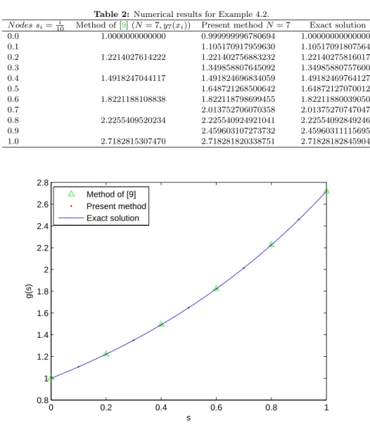
Example 4.2. Consider linear integro-differential equation [9]:
(4.2)
g′′(s) +sg′(s)−sg(s) =es+1
2scos(s)− 1 2
∫ s
0
cos(s)e−tg(t)dt ; 0≤s, t≤1,
with the initial condition g(0) = 1, g′(0) = 1 and the exact solution
g(s) =es. Table 2 and Figure 1 shows the numerical results for Example 4.2 in comparison with method of [9].
Table 2: Numerical results for Example 4.2.
N odes si=10i Method of [9] (N= 7, y7(xi)) Present methodN= 7 Exact solution
0.0 1.0000000000000 0.999999996780694 1.000000000000000
0.1 1.105170917959630 1.105170918075648
0.2 1.2214027614222 1.221402756883232 1.221402758160170
0.3 1.349858807645092 1.349858807576003
0.4 1.4918247044117 1.491824696834059 1.491824697641270
0.5 1.648721268500642 1.648721270700128
0.6 1.8221188108838 1.822118798699455 1.822118800390509
0.7 2.013752706070358 2.013752707470477
0.8 2.2255409520234 2.225540924921041 2.225540928492468
0.9 2.459603107273732 2.459603111156950
1.0 2.7182815307470 2.718281820338751 2.718281828459046
0 0.2 0.4 0.6 0.8 1 0.8
1 1.2 1.4 1.6 1.8 2 2.2 2.4 2.6 2.8
s
g(s)
Method of [9] Present method Exact solution
Figure 1. Numerical results for Example 4.2.
5. Conclusions
In this paper, solving a linear integro-differential equation became to solve a system of linear equations. To this end, the kernel of integro-differential equation and other known functions have been extended by
the least squares approximation of Legendre-Bernstein basis. Also the unknown function and its derivatives have been extended in terms of Bernstein basis. The advantage of this method is that, both character-istics orthogonality of Legendre polynomials and simplification of Bern-stein polynomials are used. Thus, we have accuracy and simplicity to-gether.Where, numerical results obtained from the examples show it. So, this basis can be used as a reliable basis for approximation func-tions.That, its coefficients are easily calculated as, it has been shown in context.
References
[1] R. T. Farouki,Legendre-Bernstein basis transformations, Comput. Appl. Math.,
119(2000), 145–160.
[2] P. J. Davis,Interpolation and approximation, New York: Dover (1975).
[3] E. Isaacson and H. B. Keller, Analysis of numerical methods, New York: Dover (1994).
[4] SA. Yousefi and M. Behroozifar,Operational matrices of Bernstein polynomials and their applications, Int. J. Syst. Sci.,41(6)(2010), 709–716.
[5] BN. Mandal and S. Bhattacharya,Numerical solution of some classes of integral equations using Bernstein polynomials, Comput. Appl. Math.,190(2007), 1707-1716.
[6] MA. Snyder,Chebychev methods in numerical approximation, Englewood Clifs; NJ. Prentice-Hall (1996).
[7] MA. Golberg and CS. Chen,Discrete projection methods for integral equations, Southampton; Comput. Mech. Publicat (1997), 178–306.
[8] Y. S¸uayip, S¸. Niyazi and Y. Ahmet, A collocation approach for solving high-order linear FredholmVolterra integro-differential equations, Math. and Compu. Model.,55(2012), 547–563.
[9] Y. S¸uayip, S¸. Niyazi and S. Mehmet, Bessel polynomial solutions of high-order linear Volterra integro-differential equations, Comput. Appl. Math.,62 (2011), 1940–1956.
Farshid Mirzaee
Department of Mathematics, Faculty of Science, Malayer University, Malayer, 65719-95863, Iran.
Email: [email protected]
Sasan Fathi
Department of Mathematics, Faculty of Science, Malayer University, Malayer, 65719-95863, Iran.