Directed Model Checking for B:
An Evaluation and New Techniques
Michael Leuschel, Jens Bendisposto Institut f¨ur Informatik, Universit¨at D¨usseldorf
Universit¨atsstr. 1, D-40225 D¨usseldorf
{leuschel, bendisposto}@cs.uni-duesseldorf.de
Abstract. ProBis a model checker for high-level formalisms such as B, Event-B, CSP and Z.ProBuses a mixed depth-first/breadth-first search strategy, and in previous work we have argued that this can perform bet-ter in practice than pure depth-first or breadth-first search, as employed by low-level model checkers. In this paper we present a thorough em-pirical evaluation of this technique, which confirms our conjecture. The experiments were conducted on a wide variety of B and Event-B models, including several industrial case studies. Furthermore, we have extended
ProBto be able to perform directed model checking, where each state is associated with a priority computed by a heuristic function. We eval-uate various heuristic functions, on a series of problems, and find some interesting candidates for detecting deadlocks and finding specific target states.
Keywords:Model Checking, B-Method, Tool Support, Directed Model Checking, Search, Industrial Case Studies,spin.
1
Introduction
Many model checking tools, such as smv [21, 3] and spin [11, 13, 2], work on relatively low-level formalisms. Recently, however, there have also been model checkers which work on higher-level formalisms, such astlc[25] for TLA+,
fdr
[9] for CSP and alloy [16] for a formalism of the same name (although the latter two are strictly speaking not model checkers). Another example isProB [19, 20] which accepts B [1].
It is relatively clear that a higher level specification formalism enables a more convenient modelling. On the other hand, conventional wisdom would dictate that a lower-level formalism will lead to more efficient model checking. However, our own experience has been different. During previous teaching and research activities, we have accumulated anecdotal evidence that using a high-level for-malism such as Bcan be much more productive than using a low-level formalism such as Promela. The study [24, 23] examined the elaboration of B models for ProB and Promela models for spin on ten different problems. Unsurprisingly, the time required to develop the Promela models was markedly higher than for the B models, (and some models could not be fully completed in Promela). The study also found out that in practice both model checkersProBandspinwere
comparable in model checking performance, despite ProBworking on a much higher-level input language and being much slower when looking purely at the number of states that can be stored and processed per time unit. Other indepen-dent experimental evaluations also report good performance ofProBcompared against SMV [15].
In [17] we first tried to analyse and understand this counter-intuitive fact. One explanation was that pure depth-first as employed by spin and other low-level model checkers fares very badly in the context of large state spaces. Similarly, a pure breadth-first strategy has problems in detecting long counter examples. We argued in [17] that ProB’s mixed depth-first/breadth-first search enabled it to effectively find a larger class of errors. In this paper we test this conjecture empirically on a large number of B specifications. In addition, we present a new directed model checking algorithm for ProB: rather than randomly choosing between doing a depth-first or breadth-first step, we associate priorities with the pending states of the model checker. We then evaluate various ways of computing priorities on the same specifications.
In Section 2 we present the motivation for mixed depth-first/breadth-first search in more detail, and in Section 3 we perform a thorough empirical eval-uation. In Section 4 we present the new directed model checking algorithm of
ProB, along with a range of heuristic functions with their empirical evaluation.
We finish with more related work and a conclusion in Section 5.
2
Combining Depth-First and Breadth-First for
Improved Model Checking
In [17] we first tried to analyse and understand the counter-intuitive behaviour described above. Below, we recall some of the conclusions from [17]. One tricky issue is the much finer granularity of low-level models. If one is not careful, the number of reachable states can explode exponentially, compared to a correspond-ing high-level model. When writcorrespond-ing Promela models, for example, great care has to be taken to make use ofatomic(or evendstep) primitives and resetting dead temporary variables to default values. However, restrictions of atomicmake it sometimes very difficult or impossible to hide all of the intermediate states. More details can be found in [17].
Searching for Errors in Large State Spaces Let us disregard the granularity issue
and let us look at simple problems, with simple datatypes, which can be easily translated from B to Promela, so that we have a one-to-one correspondence of the states of the models. In such a setting, one would assume that the spin model checker for Promela will outperformProBby several orders of magnitude. Indeed,spingenerates a specialised model checker in C which is then compiled, whereas ProB uses an interpreter written in Prolog. Furthermore, spin has accrued many optimisations over the years, such as partial order reduction [14, 22] and bitstate hashing [12]. However, even in this setting, this advantage of
in particular when using the model checker as a debugging tool for software systems, i.e., trying to find errors in a very large state space.
One experiment reported on in [17] is the NastyVendingMachine. It has a very large state space, where there is a systematic error in one of the operations of the model (as well as a deadlock when all tickets have been withdrawn). To detect the error, it is important to exercise this operation repeatedly. It is not important to generate long traces of the system, but it is important to systematically execute combinations of the individual operations. This explains why depth-first behaves so badly on this model, as it will always try to exercise the first operation of the model first. Note that a very large state space is a typical situation in software verification (sometimes the state space is even infinite).
Fortunately, spin provides a breadth-first option, with which it then finds the above error very quickly. However, for another class of problems, breadth-first fares badly. Indeed, in a corrected non-deadlocking model of the vending machine in [17], with again a large state space, the error occurs if the system runs long enough: it is not very critical in which order operations are performed, as long as the system is running long enough. This explains why for this model breadth-first was performing badly, as it was not generating traces of the system which were long enough to detect the error.
In order to detect both types of errors with a single model checking algorithm,
ProB has been using a mixed depth-first and breadth-first search [20]. More
precisely, at every step of the model checking,ProBrandomly chooses between a depth-first and a breadth-first step.
In summary, the motivation behindProB’s heuristic is that many errors in software models fall into one of the following two categories:
– Some errors are due to an error in a particular operation of the system; hence it makes sense to perform some breadth-first exploration to exercise all the available functionality. In the early development stages of a system model, this kind of error is very common.
– Some errors happen when the system runs for a long time; here it is often not so important which path is chosen, as long as the system is running long enough. An example of such an error is when a system fails to recover resources which are no longer used, hence leading to a deadlock in the long run.
Thus, if the state space is very large, depth-first search can perform very badly as it fails to systematically test combinations of the various operations of the system. Even partial order reduction and bitstate hashing often do not help. Similarly, breadth-first search can perform badly, failing to locate errors that require the system to run for very long. We have argued thatProB’s combined depth-first breadth-first search with a random component does not have these pitfalls. In the next section, we will validate this claim empirically.
3
Depth-First versus Breadth-First: An Empirical
Evaluation
We report on experiments conducted with ProB using pure depth-first, pure breadth-first, as well as the default mixed depth-first/breadth-first approach of
ProB. We also investigate several variations of the mixed approach, varying the
probability with which a depth-first step is conducted.
3.1 The Models
We have chosen a variety of case studies for evaluating the effectiveness the various model checking techniques. All models are either classical B models or Rodin Event-B models. We have included several industrial specifications (some stemming from various EU projects, such as Rodin and Deploy1), as well as
academic specifications of various intricate algorithms. There are a few artificial benchmarks as well, testing specific aspects of the model checking algorithm. We have also included some classical puzzles as well, in particular to test directed model checking.
The case studies have been partitioned into four classes: 1. Models with invariant violations,
2. Models with deadlocks,
3. Models with no errors (i.e., no deadlocks or invariant violations), but where a particular goal predicate is to be found. Indeed, in ProB the user can define a particular goal predicate and ask the model checker to find states which make the predicate true. The main difference with point 1 is that the goals are often much more precise (sometimes a concrete particular state) than the invariant violations.
4. Models with no errors, and where the full state space needs to be explored. A description of the models can be found in the extended version of the paper [18]. Along with the extended version of the paper [18] we have also included the publicly available models.
3.2 The Results
The results are summarised in Tables 1–6 in the Appendix A. Due to space restrictions, we have not included the times for the models without errors; this information can be found in [18]. Relative times are computed withProBusing a mixed depth-first/breadth-first strategy with one-third probability of going depth-first. We call this the reference settings ofProB(prior to the publication of this paper this used to be the default setting; more on that below). The experiments were run on a MacBook Pro with a 3.06 GHz Core2 Duo processor, andProB1.3.2 compiled with SICStus Prolog 4.1.2.
1
EU funded FP7 research project 214158: DEPLOY (Industrial deployment of ad-vanced system engineering methods for high productivity and dependability).
Pure Depth-First In a considerable number of cases pure depth-first is the fastest method, e.g., for the Peterson err, Abrial Earely3 v5, Alstom axl3, and BlocksWorld benchmarks.
However, we can see in Table 1 that for some models Depth-First fares very badly:
– In Alstom ex7 in Table 2, pure depth-first search even fails to find the dead-lock when given an hour of cputime. This real-life example thus supports our claim from [17] and subsection 2 that when state space is too large to examine fully, depth-first will sometimes not find a counter example. This is actually a quite common case for industrial models: they are typically (at least before abstraction) too large to handle fully.
– Another similar example is Abrial Press m13 in Table 3, where pure depth-first is about 900 times slower thanProBin the reference settings.
– Another bad example is Puzzle8, where depth-first is more than 7 times slower or Simpson4Slot where it is 163 times slower thanProBin the ref-erence settings. Finally, for the artificially constructed BFTest, depth-first search fails to find the invariant violation.
For finding goals, the geometric mean of the relative runtimes was 0.92, i.e., slightly better than the reference setting. Overall, pure depth-first seemed to fare best for the deadlocking models with a geometric mean of 0.43. For finding invariant violations, however, the geometric mean was 1.03, i.e., slightly worse than the reference setting.
The bad performance in the Huffman benchmark is actually not relevant: here not all states were evaluated. As such, the time to examine 10,000 states was measured. The pure-depth first search here encountered more complicated states, than the other approaches, explaining the additional time required for model checking.
In conclusion, the performance of pure depth-first alone can vary quite dra-matically, from very good to very bad. A such, pure depth first search is not a good choice as a default setting ofProB. Note, however, that we allow the user to override the default setting and putProBinto pure depth-first mode.
Pure Breadth-First In most cases pure Breadth-First is worse than the ref-erence setting; in some cases considerably so. The geometric mean was always above 1, i.e., worse than the reference setting.
For Alstom ex7 pure breadth-first also fails to find the deadlock.
Peterson err in Table 1 gives a similar picture, Breadth-First being 134 times slower than DF and 11 times slower than the reference settings ofProB. Other examples where BF is not so good: Abrial Earley3 v5, DiningPhil, Syste-mOnChip Router, Wegenetz.
There are some more examples where it performs considerably better than pure depth-first: Puzzle8, Simpson4Slot, Abrial Press m13 and the “artificial” benchmarks BFTest and DFTest2.
In conclusion, breadth-first on its own is not appropriate, except in special circumstances. Note, a user can setProBinto breadth-first mode, but the de-fault is another setting (see below).
Mixed Depth-first/Breadth-first The motivation behind ProB’s mixed depth-first/breadth-first heuristic is that many errors in software models fall into one of the following two categories:
– Some errors are due to an error in a particular operation of the system; hence it makes sense to perform some breadth-first exploration to exercise all the available functionality. In the early development stages of a model, this kind of error is very common.
– Some errors happen when the system runs for a long time; here it is often not so important which path is chosen, as long as the system is running long enough. An example of such an error is when a system fails to recover resources which are no longer used, hence leading to a deadlock in the long run.
An interesting real-life benchmark is Alstom ex7: here both pure depth-first and pure breadth-first fail to find the deadlock. However, the mixed strategy finds the deadlock.
We have experimented with four different versions of the mixed strategy: DF75, DF50, DF33, DF25. The reference setting was DF33, where there is a 33 % chance of going depth-first at each step. Best overall geometric mean is obtained when using DF50 (which is now the new default setting ofProB).
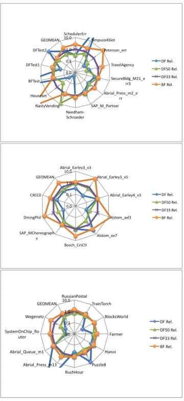
In summary, let us look at the radar plots in Table 7 in Appendix A, where we summarise the results for pure depth-first, pure breadth-first, the old reference setting and the new one. We can clearly see the quite erratic performance of pure depth-first (relative to the reference setting), and the less erratic but usually worse performance of pure breadth-first. We can also see that the new reference setting usually lies within the reference setting circle, smoothing out most of the (bad) erratic behaviour of the pure depth-first approach.
4
Evaluating Directed Model Checking
Directed Model Checking uses additional information about the model or the destination state in form of a heuristic that guides the model checker towards a target state. This additional information can be collected using for instance static analysis or it can be given by the modeler.
Currently the state space ofProBis stored as a Prolog fact database. Every state can be quickly accessed using its ID or using the hash-value of its state. The model checker also maintains a pending list of open states, using two additional Prolog predicates: retracting a Prolog fact from one of the predicates yields the most recently added open state (for depth-first traversal) and retracting from the other predicate yields the oldest open state (for breadth-first traversal). This
approach allowed us to implement a mixed depth-first / breadth-first approach by randomly selecting either an element from the front or the end of the pending list of open states.
We have implemented a priority queue in C++ using the STL (Standard Template Library) multimapdata structure. One can thus efficiently add new open states with a particular weight, and then either chose the state with the lowest or highest weight.
We now describe the various heuristic functions we have investigated, as well as the result of the empirical investigation. In this paper we evaluate some strategies to assign weights to newly encountered states. In particular we describe a random search, a search based on the number of successor states, a search based on the (term)size of the state as well as some custom heuristic functions written by the modeler for a particular model. The latter approach is used for models where a specific goal was known, e.g., puzzles.
Random Hash The idea is simply to use the hash value of a state as the weight for the priority queue. The hope is that the hash value distributes uniformly, i.e., that this would provide a good way to randomize the treatment of pending states. The hash value is computed anyway for every state, using SICStus Prolog term hash predicate.
The purpose was to use this heuristic as a base-line: a heuristic that is worse or not markedly better than this one is not worth the effort. We also want to compare this heuristic with the mixed depth-first/breadth-first approach from Section 3 and see whether there any notable differences. Indeed, the mixed depth-first/breadth-first search does not randomize the order of the states in the list, and this could have an influence on the model checking performance.
Results For finding deadlocks (Table 5) and goals (Table 6) the random hash
heuristic is markedly better than the reference settings ofProB(except for the Bosch cruise control model; but runtimes there are very low anyway). For finding invariant violations, however, (Table 4) it is worse (its geometric mean is greater than 1 (1.07) and in two examples it is markedly worse).
Overall, it seems to perform slightly better than our mixed DF/BF search. We have also experimented with truly random approach, where we use a random number generator rather than the hash value for the priority. The results are rather similar, except for Alstom ex7 where it systematically outperforms Random Hash.
Out Degree The idea is to use the out degree of a state as priority, i.e., the number of outgoing transitions. The motivation is that if we have found a state with an out degree of 0, i.e., the highest priority, we have found a deadlock. Intuitively, the less transitions are enabled for a state, the closer we may be to a deadlock. In the implementation we actually do not know the out degree of a state until it has been processed. Hence, we use the out degree of the (first) predecessor state for the priority.
Results Indeed, for finding deadlocks this heuristic obtained the best geometric mean of 0.5. So, this simple heuristic works surprisingly well. For finding goals, this heuristic still obtains geometric mean of 0.63, but it is worse than the random hash function. For finding invariant violations it does not work at all; its geometric mean is 1.56.
A further refinement of this heuristic is to combine the out degree with the random hash heuristic, i.e., if two states have the same out degree (which can happen quite often) we use the hash value as heuristic to avoid a degeneration into depth-first search. This refinement leads to a further performance improve-ment for deadlock finding (geometric mean of 0.34 compared to 0.50), and for goal finding. But it is markedly worse for invariant violation finding.
In conclusion, the out degree heuristic, especially when combined with ran-dom hash, works surprisingly well for its intended purpose of finding deadlocks. In future work, we plan to further refine this approach, by using a static flow analysis to guide model checker into deadlocks and/or particular enablings for events.
Term Size The idea of this heuristic is to use the term size of the state (i.e., the number of constant and function symbols appearing in its representation) as priority. The motivation for this heuristic is that the larger the state is, the more complicated it will be to process (for checking invariants and computing outgoing transitions). Hence, the idea is to process simpler states first, in an attempt to maximise the number of states processed per time unit.
Results For finding goals this heuristic has a geometric mean of 0.85, i.e., it is
better than the reference setting of ProB, but worse than random hash. For deadlock and invariant checking, it also performs worse than random hash. In summary, this heuristic does not seem worth pursuing further.
Effectiveness of Custom Heuristic Function: In order to experiment easily with other heuristic functions, we have added the possibility for the user to define a custom heuristic function for a B model. Basically, this function can be intro-duced in the DEFINITIONS part of a B machine by definingHEURISTIC FUNCTION.
ProB now evaluates the expression HEURISTIC FUNCTION in every state, and uses its value as the priority of the state. Note, the expression must return an integer value. For the BlocksWorld benchmark, we have written the following custom heuristic function:
ongoal == {a|->b, b|->c, c|->d, d|->e};
DIFF(A,TARGET) == (card(A-TARGET) - card(TARGET /\ A)); HEURISTIC_FUNCTION == DIFF(on,ongoal);
Note the machine has a variableonis of typeObjects +-> Objectsand the GOAL for the model checker is to find a state whereon = ongoal is true.
In the benchmarks, we have mainly written heuristic functions which esti-mate the distance between a target goal state and the current state. In future,
we plan to derive the definition of those heuristic functions automatically. A simple distance heuristic can be derived if the goal of the model checking is to find specific values for certain variables of the machine (such as on = ongoal). Basically, for current states=hs1, . . . , sniand a target statet=ht1, . . . , tniwe
use as heuristich(s) = Σ1≤i≤n∆(si, ti) where
– ∆(x, target) =abs(x−target) ifxinteger
– ∆(x, target) = card(x−T ARGET)−card(T ARGET∩A) ifxa set – ∆((x, y),(t1, t2)) =∆(x, t1) +∆(y, t2) for pairs,
– in all other cases:∆(x, target) = 0 ifx=target and 1 otherwise
If the value of a particular variable is not relevant, then we simply set∆(si, ti) =
0 for that variable.
This defines a kind of Hamming distance for B states. We have applied this (manually) in the BlocksWorld example above.
We have only evaluated this approach for finding goals. Here, it obtained the best overall geometric mean of 0.34. For Puzzle8 and Abrial press m13, this approach yielded by far the best solution. For RussianPostal, TrainTorch, Blocksworld, Abrial Queue m1 it obtains the best result. There was one exper-iment were it is markedly worse than ProB in the reference settings: Syste-mOnChip Router. Here the heuristic did not pay off at all. Indeed, here the last event changes all of the four variables, relevant for the model checking GOAL, in one step. This only confirms the fact that we are working withheuristic func-tions, which are not guaranteed to always improve the performance.
Summary of the Directed Model Checking Experiments: We have sum-marised the main findings of our experiments in Table 8 in Appendix A. We can conclude that:
– for invariant checking, the random hash heuristic fared best.2 This seems to indicate that it is maybe useful to combine some more random component into the depth-first/breadth-first techniques of Section 3, e.g., to also ran-domly permute the operation order. Indeed, the approaches from Section 3 always process the operations in the same order, and do not shuffle the states inside the pending list.
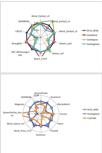
– for deadlock checking, the out-degree-hash heuristic is the best. It should provide a good basis for further improved deadlock checking techniques. – for goal finding, a custom heuristic function provides (except in one case)
by far the best result. The next step is to derive those heuristic functions automatically.
The out-degree-hash heuristic also provides reasonably good performance (its geometric mean is 0.41, which is better than the best mixed-depth-first one of 0.57 for DF75).
2
However, note that DF50 had an overall geometric mean of 0.58, and was hence better overall than random hash.
5
Future and Related Work and Conclusion
Regarding directed model checking using heuristics there are a number of other approaches such as a directed extension [10] for Java PathFinder, a tool to mod-elcheck Java bytecode in order to find deadlocks or problems with null pointers. Edelkamp et al. describe in [7, 6, 5] various methods to do directed searches for counterexamples to LTL properties within spin. A way to use abstraction in order to direct a model checker is described in [4].
Our experiments have confirmed the conjecture of [17], namely that a mixed depth-first/breadth-first strategy for model checking is much more robust than either pure depth-first or breadth-first search. Of particular interest is one indus-trial model (from Alstom), where neither pure depth-first nor pure breadth-first was capable of detecting the deadlock. We have presented a new model checking algorithm forProB, which stores the pending list of states in a priority queue. We have presented several heuristic functions and have evaluated them on a wide variety of B models, including several industrial case studies. The experiments have shown that directed model checking can provide a considerable performance improvement. We have shown how one technique, combining the out-degree with a random component, performs very well for finding deadlocks. An adaption of the hamming distance for B states has proven to be very effective in guiding the model checker towards specific goal predicates.
In the future we want to develop more intelligent heuristic functions to guide
ProB, e.g., using information we get from an automatic flow analyzer. We
cur-rently investigate a method to extract information about the control flow of software systems from Event-B models using a theorem prover. We hope that flow analysis guided model checking will further improve upon the out-degree heuristic for finding deadlocks and would also be helpful to find traces to states where a particular event is enabled. The latter is particularly interesting for test-case generation.
Acknowledgements We would like to thank the SBMF reviewers for their
feed-back and many useful suggestions. We are also grateful to the various industrial partners for giving us access to their B models. This research is being carried out as part of the DFG funded research project GEPAVAS and the EU funded FP7 research project 214158: DEPLOY (Industrial deployment of advanced system engineering methods for high productivity and dependability).
References
1. J.-R. Abrial. The B-Book. Cambridge University Press, 1996. 2. M. Ben-Ari. Principles of the Spin Model Checker. Springer, 2008.
3. J. R. Burch, E. M. Clarke, K. L. McMillan, D. L. Dill, and L. J. Hwang. Symbolic model checking: 1020states and beyond.Information and Computation, 98(2):142– 170, Jun 1992.
4. K. Dr¨ager, B. Finkbeiner, and A. Podelski. Directed model checking with distance-preserving abstractions. In A. Valmari, editor, SPIN, LNCS 3925, pages 19–34. Springer, 2006.
5. S. Edelkamp and S. Jabbar. Large-scale directed model checking LTL. In A. Val-mari, editor,SPIN, LNCS 3925, pages 1–18. Springer, 2006.
6. S. Edelkamp, S. Leue, and A. Lluch-Lafuente. Directed explicit-state model check-ing in the validation of communication protocols. STTT, 5(2-3):247–267, 2004. 7. S. Edelkamp, S. Leue, and A. Lluch-Lafuente. Partial-order reduction and trail
improvement in directed model checking. STTT, 6(4):277–301, 2004.
8. P. J. Fleming and J. J. Wallace. How not to lie with statistics: the correct way to summarize benchmark results. Commun. ACM, 29(3):218–221, 1986.
9. Formal Systems (Europe) Ltd. Failures-Divergence Refinement — FDR2 User Manual (version 2.8.2).
10. A. Groce and W. Visser. Heuristic model checking for Java programs. In D. Bosnacki and S. Leue, editors, SPIN, LNCS 2318, pages 242–245. Springer, 2002.
11. G. J. Holzmann. The model checker Spin. IEEE Trans. Software Eng., 23(5):279– 295, 1997.
12. G. J. Holzmann. An analysis of bitstate hashing. Formal Methods in System Design, 13(3):289–307, 1998.
13. G. J. Holzmann.The Spin Model Checker: Primer and Reference Manual. Addison-Wesley, 2004.
14. G. J. Holzmann and D. Peled. An improvement in formal verification. In D. Hogrefe and S. Leue, editors,FORTE, volume 6 ofIFIP Conference Proceedings, pages 197– 211. Chapman & Hall, 1994.
15. T. H¨orne and J. A. van der Poll. Planning as model checking: the performance of ProB vs NuSMV. In R. Botha and C. Cilliers, editors,SAICSIT Conf., volume 338 ofACM International Conference Proceeding Series, pages 114–123. ACM, 2008. 16. D. Jackson. Alloy: A lightweight object modelling notation. ACM Transactions
on Software Engineering and Methodology, 11:256–290, 2002.
17. M. Leuschel. The high road to formal validation. In E. B¨orger, M. Butler, J. P. Bowen, and P. Boca, editors,Proceedings ABZ 2008, LNCS 5238, pages 4–23, 2008. 18. M. Leuschel and J. Bendisposto. Directed model checking for B: An evaluation and new techniques. Technical report, STUPS, Universit¨at D¨usseldorf, September 2010. Available at http://www.stups.uni-duesseldorf.de/publications detail.php?id=312. 19. M. Leuschel and M. Butler. ProB: A model checker for B. In K. Araki, S. Gnesi,
and D. Mandrioli, editors,FME 2003: Formal Methods, LNCS 2805, pages 855–874. Springer-Verlag, 2003.
20. M. Leuschel and M. J. Butler. ProB: an automated analysis toolset for the B method. STTT, 10(2):185–203, 2008.
21. K. L. McMillan. Symbolic Model Checking. PhD thesis, Boston, 1993.
22. D. Peled. Combining partial order reductions with on-the-fly model-checking. In D. L. Dill, editor,CAV, LNCS 818, pages 377–390. Springer, 1994.
23. M. Samia, H. Wiegard, J. Bendisposto, and M. Leuschel. High-Level versus Low-Level Specifications: Comparing B with Promela and ProB with Spin. In Attiogbe and Mery, editors,Proceedings TFM-B 2009, pages 49–61. APCB, June 2009. 24. H. Wiegard. A comparison of the model checker ProB with Spin. Master’s thesis,
Institut f¨ur Informatik, Universit¨at D¨usseldorf, 2008. Bachelor’s Thesis.
25. Y. Yu, P. Manolios, and L. Lamport. Model checking TLA+ specifications. In L. Pierre and T. Kropf, editors, CHARME, LNCS 1703, pages 54–66. Springer, 1999.
A
Experimental Results
Note: we use geometric mean [8] of the relative runtimes, as the arithmetic mean is useless for normalised results. Of course, the geometric mean itself should also be taken with a grain of salt (various articles also attack its usefulness). Indeed, without knowing how representative the chosen benchmarks are for the overall population of B specifications, we can conclude little.
Thus, we also provide all numbers in the tables below, so that minimum, maximum relative runtimes can be seen, as well as the absolute runtime of the reference benchmark. Indeed, the relative runtimes are less reliable, when the absolute runtime of the reference benchmark is already very low. When a given technique failed to locate the invariant violation (respectively deadlock or target goal), then we have marked the time with two asterisks (**). The tables for the models without errors where the full state space has to be explored can be found in [18].
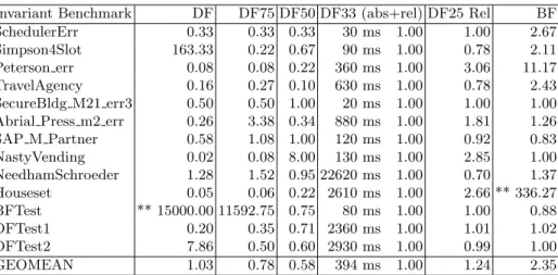
Invariant Benchmark DF DF75 DF50 DF33 (abs+rel) DF25 Rel BF
SchedulerErr 0.33 0.33 0.33 30 ms 1.00 1.00 2.67
Simpson4Slot 163.33 0.22 0.67 90 ms 1.00 0.78 2.11 Peterson err 0.08 0.08 0.22 360 ms 1.00 3.06 11.17 TravelAgency 0.16 0.27 0.10 630 ms 1.00 0.78 2.43 SecureBldg M21 err3 0.50 0.50 1.00 20 ms 1.00 1.00 1.00 Abrial Press m2 err 0.26 3.38 0.34 880 ms 1.00 1.81 1.26 SAP M Partner 0.58 1.08 1.00 120 ms 1.00 0.92 0.83 NastyVending 0.02 0.08 8.00 130 ms 1.00 2.85 1.00 NeedhamSchroeder 1.28 1.52 0.95 22620 ms 1.00 0.70 1.37 Houseset 0.05 0.06 0.22 2610 ms 1.00 2.66 ** 336.27 BFTest ** 15000.00 11592.75 0.75 80 ms 1.00 1.00 0.88 DFTest1 0.20 0.35 0.71 2360 ms 1.00 1.01 1.02 DFTest2 7.86 0.50 0.60 2930 ms 1.00 0.99 1.00 GEOMEAN 1.03 0.78 0.58 394 ms 1.00 1.24 2.35
Deadlock Benchmark DF DF75 DF50 DF33 (abs+rel) DF25 Rel BF Abrial Earley3 v3 0.33 0.44 0.93 270 ms 1.00 1.19 1.19 Abrial Earley3 v5 0.13 0.32 0.75 4320 ms 1.00 2.18 7.95 Abrial Earley4 v3 0.89 0.89 1.00 90 ms 1.00 1.00 1.00 Alstom axl3 0.10 0.17 0.20 51270 ms 1.00 3.51 14.61 Alstom ex7 ** 4.20 0.23 0.35 856320 ms 1.00 ** 1.21 ** 3.00 Bosch CrsCtl 1.00 1.00 1.00 3 ms 1.00 4.00 4.00 SAP MChoreography 0.50 0.50 0.50 20 ms 1.00 1.00 1.00 DiningPhil 0.13 0.26 0.36 1690 ms 1.00 2.49 6.20 CXCC0 0.50 1.00 1.00 10 ms 1.00 2.00 2.00 GEOMEAN 0.43 0.44 0.59 540 ms 1.00 1.82 3.02 AVG 0.00 0.00 0.00 0 ms 0.00 0.00 0.00
Table 2.Relative times for checking models with deadlocks (DF/BF Analysis)
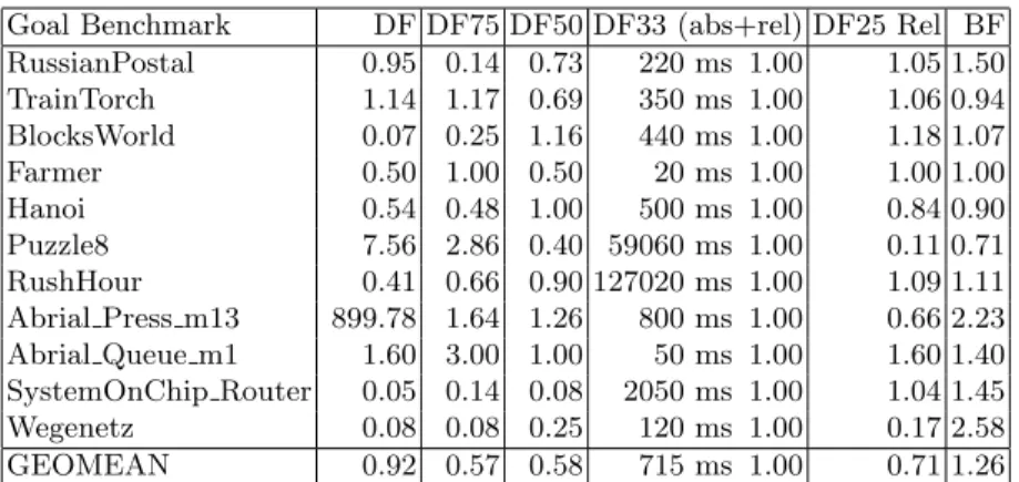
Goal Benchmark DF DF75 DF50 DF33 (abs+rel) DF25 Rel BF RussianPostal 0.95 0.14 0.73 220 ms 1.00 1.05 1.50 TrainTorch 1.14 1.17 0.69 350 ms 1.00 1.06 0.94 BlocksWorld 0.07 0.25 1.16 440 ms 1.00 1.18 1.07 Farmer 0.50 1.00 0.50 20 ms 1.00 1.00 1.00 Hanoi 0.54 0.48 1.00 500 ms 1.00 0.84 0.90 Puzzle8 7.56 2.86 0.40 59060 ms 1.00 0.11 0.71 RushHour 0.41 0.66 0.90 127020 ms 1.00 1.09 1.11 Abrial Press m13 899.78 1.64 1.26 800 ms 1.00 0.66 2.23 Abrial Queue m1 1.60 3.00 1.00 50 ms 1.00 1.60 1.40 SystemOnChip Router 0.05 0.14 0.08 2050 ms 1.00 1.04 1.45 Wegenetz 0.08 0.08 0.25 120 ms 1.00 0.17 2.58 GEOMEAN 0.92 0.57 0.58 715 ms 1.00 0.71 1.26
Table 3.Relative times for checking models with goals to be found (DF/BF Analysis)
Invariant Benchmarks DF33 (abs+rel) HashRand OutDegree OutDegHash TermSize
SchedulerErr 30 ms 1.00 0.33 3.67 10.67 2.67
Simpson4Slot 90 ms 1.00 0.89 2.22 0.78 2.22
Peterson err 360 ms 1.00 0.75 11.25 1.42 9.14
TravelAgency 630 ms 1.00 0.52 1.02 9.98 0.49
SecureBldg M21 err3 20 ms 1.00 0.50 1.00 0.50 0.50 Abrial Press m2 err 880 ms 1.00 1.45 3.38 3.19 1.25
SAP M Partner 120 ms 1.00 1.17 0.75 0.33 1.00 NeedhamSchroeder 22620 ms 1.00 1.40 **48.51 41.58 ** 46.06 Houseset 2610 ms 1.00 0.08 ** 333.53 0.16 ** 338.61 BFTest 80 ms 1.00 16.00 0.88 73.00 0.88 DFTest1 2360 ms 1.00 0.64 1.02 0.69 1.02 DFTest2 2930 ms 1.00 0.53 1.00 0.57 1.66 GEOMEAN 432 ms 1.00 0.79 2.44 1.54 1.93
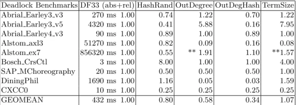
Deadlock Benchmarks DF33 (abs+rel) HashRand OutDegree OutDegHash TermSize Abrial Earley3 v3 270 ms 1.00 0.74 1.22 0.70 1.22 Abrial Earley3 v5 4320 ms 1.00 0.41 5.88 0.16 7.95 Abrial Earley4 v3 90 ms 1.00 0.89 1.00 0.89 1.00 Alstom axl3 51270 ms 1.00 0.82 0.09 0.16 0.08 Alstom ex7 856320 ms 1.00 0.55 ** 1.91 1.10 **1.57 Bosch CrsCtl 3 ms 1.00 8.00 1.00 1.00 4.00 SAP MChoreography 20 ms 1.00 0.50 0.50 0.50 1.00 DiningPhil 1690 ms 1.00 1.16 0.05 0.03 1.59 CXCC0 10 ms 1.00 0.25 0.25 0.25 0.25 GEOMEAN 432 ms 1.00 0.80 0.58 0.34 1.07
Table 5.Relative times for checking models with deadlocks (Heuristics Analysis)
Goal DF33 HashRand OutDegree OutDeg- TermSize CUSTOM
Benchmarks (abs+rel) Hash
RussianPostal 220 ms 1 0.45 0.77 0.36 1.18 0.45 TrainTorch 350 ms 1 0.97 0.26 1.14 0.20 0.20 BlocksWorld 440 ms 1 1.16 0.07 0.07 1.20 0.02 Farmer 20 ms 1 1.00 1.00 0.50 1.00 1.00 Hanoi 500 ms 1 0.52 0.92 0.52 0.90 0.34 Puzzle8 59060 ms 1 20.54 1.31 2.69 0.71 0.03 RushHour 127020 ms 1 0.42 0.60 0.56 1.12 0.79 Abrial Press m13 800 ms 1 0.49 2.36 2.21 2.48 0.20 Abrial Queue m1 50 ms 1 0.40 16.60 0.60 2.80 0.40 SystemOnChip... 2050 ms 1 0.10 0.05 0.04 1.50 72.42 Wegenetz 120 ms 1 0.17 0.33 0.08 0.08 0.08 GEOMEAN 715 ms 1 0.64 0.63 0.41 0.85 0.34
0.0 0.1 1.0 10.0 SchedulerErr Simpson4Slot Peterson_err TravelAgency SecureBldg_M21_e rr3 Abrial_Press_m2_e rr SAP_M_Partner Needham-‐ Schroeder NastyVending Houseset BFTest DFTest1 DFTest2 GEOMEAN DF Rel. DF50 Rel. DF33 Rel. BF Rel. 0.0 0.1 1.0 10.0 Abrial_Earley3_v3 Abrial_Earley3_v5 Abrial_Earley4_v3 Alstom_axl3 Alstom_ex7 Bosch_CrsCtl SAP_MChoreograph y DiningPhil CXCC0 GEOMEAN DF Rel. DF50 Rel. DF33 Rel. BF Rel. 0.0 0.1 1.0 10.0 RussianPostal TrainTorch BlocksWorld Farmer Hanoi Puzzle8 RushHour Abrial_Press_m13 Abrial_Queue_m1 SystemOnChip_Ro uter Wegenetz GEOMEAN DF Rel. DF50 Rel. DF33 Rel. BF Rel.
0.01 0.10 1.00 Abrial_Earley3_v3 Abrial_Earley3_v5 Abrial_Earley4_v3 Alstom_axl3 Alstom_ex7 Bosch_CrsCtl SAP_MChoreogra phy DiningPhil CXCC0 GEOMEAN DF33_BF66 HashRand OutDegree OutDegHash 0.01 0.10 1.00 10.00 RussianPostal TrainTorch BlocksWorld Farmer Hanoi Puzzle8 RushHour Abrial_Press_m13 Abrial_Queue_m1 SystemOnChip_Rou ter Wegenetz GEOMEAN DF33_BF66 OutDegHash CUSTOM