Social Security Reform with Heterogeneous Mortality
John Bailey Jones
Yue Li
∗July 17, 2020
Abstract
Using a heterogeneous agent, life-cycle model of Social Security claiming, labor supply and saving, we consider the implications of lifespan inequality for Social Security reform. Quantitative experiments show that welfare is maximized when baseline benefits are independent of lifetime earnings, the payroll tax cap is kept roughly unchanged, and claiming adjustments are reduced. Eliminating the earnings test and the income taxation of Social Security benefits provides additional gains. The Social Security system that would maximize welfare in a “2050 demographics” scenario, characterized by longer lifespans and an increased education-mortality gradient, is similar to the one that would maximize welfare today.
JEL: E21, H24, H55, I38, J11
Keywords: Social Security, Mortality, Labor Supply, Welfare
∗John Bailey Jones: Federal Reserve Bank of Richmond, john.jones@rich.frb.org. Yue Li: University
at Albany, SUNY, yli49@albany.edu. For helpful comments, we thank seminar participants at American University, University of Houston, William and Mary, the ESRC Conference on Inequality and the Insur-ance Value of Transfers over the Life Cycle and the U.S.C FBE Workshop on the Economics of Health and Aging. The research reported herein was performed pursuant to grant RDR18000003 from the U.S. Social Security Administration (SSA) funded as part of the Retirement and Disability Research Consortium. The opinions and conclusions expressed are solely those of the author(s) and do not represent the opin-ions or policy of SSA, any agency of the Federal Government, NBER, Federal Reserve Bank of Richmond or the Federal Reserve System. Neither the U.S. Government nor any agency thereof, nor any of their employees, makes any warranty, express or implied, or assumes any legal liability or responsibility for the accuracy, completeness, or usefulness of the contents of this report. Reference herein to any specific commercial product, process or service by trade name, trademark, manufacturer, or otherwise does not necessarily constitute or imply endorsement, recommendation or favoring by the U.S. Government or any agency thereof.
1
Introduction
One of the most common proposals for stabilizing the Social Security system is to increase the normal retirement age (NRA). An appealing feature of this proposal is that it counters the secular trend toward longer lives, a major cause of Social Security’s financial difficulties, by effectively delaying the age at which full benefits start. It is also well-known, however, that the longevity gap between rich and poor is large and growing over time (National Academies of Sciences, Engineering, and Medicine 2015; Chetty et al. 2016). This has generated concerns that raising the NRA would cut disproportionately the benefits of the poor (e.g., Krugman 2015). While these concerns can be mitigated by changing the progressivity of the benefit formula (Cremer et al., 2010), the more general question remains. If high-income workers live longer than low-income workers, should they work longer as well? Should they receive higher annual benefits?
When considering such questions, several conflicting principles come into play. (Cre-mer et al. 2010 provide a nice encapsulation. See also Ndiaye 2018.) Mirrlees’s (1971) canonical framework highlights the tension between equalizing consumption and encour-aging work by the most productive. In our setting, this implies that high-productivity workers should retire at older ages. With heterogeneous mortality, “equal consumption” must be defined as well. Solutions to social planners’ problems often involve equating the weighted marginal utility of consumption across all surviving agents. This can imply equal per-period consumption flows, but larger lifetime transfers to the long-lived. Inevitably, optimal pension design is a quantitative exercise.
To examine these issues, we develop a heterogeneous-agent, life-cycle model of Social Security claiming, labor supply and saving. In the model, individuals face uncertain health, wages, medical spending and survival, the distributions of which vary by education level. The government collects income, payroll and consumption taxes, and provides Social Security, Medicare, Disability Insurance and means-tested social insurance. Individuals
can continue working while receiving Social Security benefits, but they may face financial disincentives to do so. After calibrating the model to the current U.S. economy and Social Security rules, we evaluate potential reforms.
In particular, we solve the following planning problem. Consider a stationary cross-sectional distribution of individuals that differ along a variety of demographic and eco-nomic dimensions. Holding fixed both aggregate Social Security expenditures and rev-enues, and maintaining general government budget balance, what are the Social Security rules that maximize the ex-ante utility of a newborn? We consider three sets of parametric reforms:
1. Changes to the payroll tax earnings cap and tax rate.
2. Changes to the formula converting an individual’s earnings history to his baseline benefit (the Primary Insurance Amount, or PIA).
3. Changes to the trade-off between the age at which an individual first receives her Social Security benefits – and thus the length of the benefit stream – and the size of the annual benefit. Increases in the NRA can be interpreted as a special case. This trade-off is formally embodied in the early retirement penalties and delayed retirement credits, which increase or decrease an individual’s annual benefits pro-portionally to his PIA.
All of the reforms that we study have appeared before as proposals, enacted changes or both. While the first two sets of reforms affect how Social Security benefits depend on wage realizations and work decisions, the third affects how benefits depend on claiming
decisions. Because individuals can simultaneously work and receive Social Security ben-efits, their work and claiming decisions may appear to be disconnected. This is not the case, however, because the rate at which earnings translate into Social Security benefits is a function of the age at which the benefits are claimed and because benefit receipt itself generates work disincentives. These disincentives include benefit reductions through the Social Security earnings test and the way in which the income taxation of Social Security benefits increases the income taxation of earnings (Jones and Li, 2018).
Each set of reforms embodies the canonical trade-off between redistribution and pro-ductive efficiency. Raising the payroll tax cap lowers the tax rate but applies it to a broader range of earnings. This reduces taxes for most workers but raises marginal tax rates for the most productive. Linking Social Security benefits to lifetime earnings in-creases the returns to work but reduces transfers from high to low earners. Raising the returns to delayed claiming rewards longer careers but punishes those with low longevity. Our general finding is that, relative to the Social Security policies currently in place, the policies that would maximize welfare would reduce work incentives in order to re-distribute resources from high to low earners. Under these policies, the PIA would be independent of lifetime earnings, and claiming adjustments would be smaller, while the upper bound on taxable earnings would remain at more or less its current value. Col-lectively the reforms cause both earnings and employment to fall by 1-2%. We show, however, that eliminating the earnings test and the income taxation of Social Security benefits, as recommended by Jones and Li (2018), reverses more than two-thirds of the fall in earnings and more than half of the fall in employment. Combining the two sets of reforms also results in larger welfare gains. Because the earnings test and benefit taxa-tion apply at older ages, when the elasticity of labor supply is especially high (French and Jones 2012; Karabarbounis 2016; Ndiaye 2018), eliminating them is an especially effec-tive way to encourage work. Removing the provisions uncouples claiming decisions from retirement decisions; under the joint reforms, almost everyone claims benefits at age 62.
We then consider how heterogeneous mortality affects Social Security reform in the face of population aging. We construct a hypothetical “2050 demographics” scenario characterized by longer lifespans, lower population growth and an increased education-mortality gradient. We find that the Social Security system that would maximize welfare in the 2050 demographic environment is quite similar to the one that would maximize welfare today. In both cases, the PIA would be independent of individual earnings; the payroll tax cap would be higher in 2050 than at present; but the claiming adjustments
would not. Although increased longevity suggests that larger claiming adjustments are needed to promote longer careers, increased longevity also implies that the adjustments needed to induce claiming delays (and longer careers) are smaller.
The literature on Social Security reforms is immense (see, e.g., Feldstein and Liebman 2002). In their review, B¨orsch-Supan et al. (2016) contrast “parametric” reforms, where the basic design of the system is unchanged, with more fundamental “systemic” reforms, such as the switch from a pay-as-you-go to a fully funded system. We restrict ourselves to parametric reforms, holding fixed Social Security’s “aggregate footprint.”1 Because the
absolute size of a country’s Social Security system can have first-order effects on its ag-gregate capital stock, our approach allows us to focus on distributional concerns. Within the literature on parametric reforms, our contribution is to consider all the reforms simul-taneously, quantitatively, and while accounting for heterogeneity in income and health. Our exercise also stands out in its breadth: among other possibilities, we consider flat benefits and what is effectively a single claiming age.
While it has been long recognized that heterogeneous mortality affects the lifetime progressivity of Social Security (Aaron, 1977), and multiple studies have sought to quan-tify this effect (recent analyses include Goda et al. 2011; Bosworth and Burke 2014; National Academies of Sciences, Engineering, and Medicine 2015; and Sheshinski and Caliendo 2018), there has been relatively little progress in quantifying its implications for optimal policies. Laun et al. (2019) and S´anchez-Romero et al. (2019) consider how to maintain fiscal sustainability in the presence of heterogeneous demographic change. (Also see Conesa et al. 2019.) Although set in Norway, the structure of Laun et al.’s (2019) model is quite similar to ours. However, they focus on a handful of reforms, including some that change the pension system’s aggregate footprint, while we seek optimal policies
1An alternative approach used in the literature is to fix tax rates and require that benefit changes
maintain Social Security budget balance (e.g., Huggett and Ventura 1999; Nishiyama and Smetters 2008; Bagchi 2019). When operating within a stationary demographic environment, this constraint is much the same as ours. The two constraints differ if one considers responses to major demographic changes.
with the footprint held fixed. S´anchez-Romero et al. (2019) consider systemic reforms in a general equilibrium framework with no health or wage uncertainty. Using a life-cycle model with heterogeneous mortality rates, Bagchi (2019) examines reforms to the Social Security benefit formula, but he does not consider claiming decisions. As we show below, claiming decisions and retirement decisions are at times closely linked, and changing the claiming adjustments is one of our principal reforms. Huggett and Ventura (1999) and Nishiyama and Smetters (2008), who also consider reforms to the benefit formula, do not allow for claiming decisions or heterogeneous mortality risk.
Huggett and Parra (2010) find the system of life-cycle taxes that implements the social planner’s solution for a cohort of individuals, holding fixed the net resources extracted from that cohort. In a separate exercise, they find that the optimal Social Security benefit function, if considered in isolation, would decrease modestly in lifetime earnings. Ndiaye (2018) expands Huggett and Parra’s (2010) framework to include a retirement choice. He finds that the optimal Social Security system would tie benefits more closely to earnings and strengthen the claiming adjustments. Huggett and Parra (2010) and Ndiaye (2018) show that Social Security reforms in isolation recover only a portion of the utility gains achievable under an optimal tax system. On the other hand, to make their exercise tractable, they impose a number of simplifications. Among the most important of these are the assumptions that all agents share a common, fixed lifespan and that agents receiving Social Security benefits are unable to work. In our robustness exercises, we show that these restrictions increase the sensitivity of retirement to claiming incentives and thus favor large claiming adjustments.
The remainder of the paper is organized as follows. In Section 2, we describe our model, while in Section 3, we describe its calibration. In Section 4, we present the policies that would maximize welfare in the current demographic environment. In Section 5, we discuss the 2050 demographic environment and the policies that would maximize welfare therein. In Section 6, we perform a number of robustness exercises. We conclude in
Section 7.
2
Model
Our behavioral model is similar to those of Imrohoro˘glu and Kitao (2012) and Jones and Li (2018) but contains a considerably richer treatment of health, mortality and wages, including heterogeneity related to education. Our description borrows heavily from Jones and Li (2018).
2.1
Demographics
The population consists of overlapping generations. Each period represents two years. Let j ∈ {1,2, . . . , J} denote age, where J represents the maximum lifespan. The popu-lation grows at the constant rate χ. Among other dimensions, new individuals differ in terms of education level (e). We assume the distribution of education is exogenous and constant over time.
Let sj(hj, e) denote the survival rate between periods, which depends on each
indi-vidual’s age, health status (hj), and education level. Health can take on five potential
values: good (hj = 1), bad (hj = 2), work limitation (hj = 3), in a nursing home (hj = 4),
and disabled (hj = 5). Health status affects individuals through five channels: the time
endowment, the survival probability, health transitions, medical expenditures, and access to Disability Insurance (DI). We assume that all individuals in the disabled health state receive DI – our empirical definition of the disability state is DI receipt – and thus ab-stract away from the DI application decision and uncertainty over DI receipt. Because the reforms we consider are not intended for the disabled, we view this as a reasonable simplification.
2.2
Preferences
Each period surviving individuals receive utility from consumption (c) and leisure (l) according to the function u(c, l). Leisure in turn depends on hours of work, nj, health,
and labor market participation in the previous period (nj−1):
lj = 1− X k φhkeI{hj=k}−φneI{nj>0}−φ reI {nj−1=0 andnj>0}−nj, (1)
where IA is the 0-1 indicator function that takes the value of 1 when event A occurs. The term φh
keI{h=k} reflects the time cost of being in health status k for a person with
education level e. This cost is normalized to 0 for individuals in good health and is intended to reproduce the empirical observation that unhealthy people work less. The term φn
eI{n>0} captures the fixed time costs of work for education level e. This term is
intended to reproduce the observation that most people work full-time or not at all (see, e.g., Cogan 1981 and French and Jones 2012). The termφreI{nj−1=0 andnj>0} captures the
time cost of reentering the labor market. Similar specifications for leisure have been used in, among other studies, French (2005) and French and Jones (2011). We assume that disabled individuals and nursing home residents cannot work.
When they die, individuals receive warm-glow utility from bequests according to the function v(a), where a denotes the amount of assets bequeathed. Future utility is dis-counted using the factor β.
2.3
Earnings
Individuals that work at age j receive the wage wj,
wj =ω(e, j, hj)·ηj·min 1,nj ¯ n ζ . (2)
Wages depend on age, education and health through ω(e, j, hj). ηj is an idiosyncratic
productivity shock following a Markov process with transitions Πηj(e, ηj, ηj+1). The final
term, min{1,[nj/n]ζ}, imposes a penalty for working less than the full-time work load of ¯n.
Following Aaronson and French (2004), we setζ to 0.415, implying that half-time workers are paid 25% less than full-time workers. Imposing the part-time earnings adjustment leads total earnings, Wj = wjnj, to have increasing returns to scale in hours of work.
This feature combines with the fixed time cost of work to encourage full-time work.
2.4
Medical Expenditures and Health Insurance
Each individual’s health status (hj) changes stochastically over the life cycle, following
a Markov process with the age-dependent transition probability πh
j(hj+1|e, hj). Total
medical expenditures, denoted by mj = mj(hj, j), depend on age, current health and
the shock j, an i.i.d. process with the stationary distribution Π(). Health insurance
coverage is universal: Medicare covers DI recipients (after a two-year waiting period) and all individuals 65 and older (j ≥JM), and private health insurance covers the rest of the population.2 The medical expenses paid by the individuals themselves can be split into two parts: insurance premia,pj, which are paid at the beginning of each period before the
medical spending shocks for that period are revealed; and co-payments, Qj(hj, j), which
are paid at the end of each period after the shocks are revealed. Premia and co-payments follow pj = ppriv if j < JM and hj−1 6= 5 pmcr+psupp otherwise, Qj(hj−1, hj, j) = (1−κpriv)m j(hj, j) if j < JM and hj−1 6= 5 (1−κmcr−κsupp)m j(hj, j) otherwise,
2The model abstracts from heterogeneity in private insurance access. Dynamic models with variable
insurance eligibility and insurance take-up include Jeske and Kitao (2009) and Pashchenko and Pora-pakkarm (2013).
where the superscripts “priv”, “mcr”, and“supp” denote, respectively, private insurance, Medicare, and Medicare supplement insurance plans. κi, i ∈ {priv,mcr,supp} is the
insurer payment rate for insurance type i.
2.5
Government
The government collects taxes and provides social insurance. The difference between the government’s revenues and its transfer spending is absorbed by direct spending (G). We assume further that the government collects all bequests, which it then distributes equally among surviving individuals, giving each the transfer B. This commonly-used,3 if clearly counterfactual, assumption simplifies the model greatly.
Old-Age Insurance (OAI). Let JE denote the Early Retirement Age (ERA), JN
denote the Normal Retirement Age (NRA), and JL denote the Late Retirement Age
(LRA). Individuals not receiving DI benefits (hj 6= 5) can choose any age from the ERA
of 62 to the LRA of 70 to claim their Social Security benefits. OAI recipients receive benefits according to Akss(Ej), where: Ak, is an adjustment factor based on the benefit
claiming age k, designed to capture early retirement penalties and delayed retirement credits; Ej is an index of the individual’s 35 highest years of earnings, commonly known
as Average Indexed Monthly Earnings (AIME); andss(·) is a function that converts the earnings index into the Primary Insurance Amount (PIA).
Beneficiaries who are below the NRA and have labor income in excess of the earning limit yet
j have their benefits withheld at a rate of τjet: for each additional dollar earned,
Social Security benefits are reduced by τjet, until all benefits are withheld. LetTjetdenote benefits lost through the earnings test, and let ss∗j denote the remaining benefits. We have
Tjet(ssj, Wj) = min
ssj, τjetmax{0, Wj−yetj } , (3)
ss∗j(ssj, Wj) =ssj−Tjet(ssj, Wj). (4)
Any such reductions in current benefits, however, are offset by permanent increases in future benefits, implemented in our framework through increases inEj+1.4 The net
incen-tive generated by the earnings test depends on whether the increases in future benefits are actuarially fair; because the current crediting formula is considered actuarially fair for the average person, for most workers the net tax rate associated with the earnings test is small.
Social Security benefits are also subject to income taxes. An important feature of these taxes is that the amount of Social Security benefits subject to taxation is increasing in the beneficiaries’ total income. At certain income levels, each additional dollar of earnings, in addition to being taxable itself, adds 50-85 cents of Social Security benefits to taxable income, increasing the effective marginal income tax rate on these earnings by 50% to 85%. Jones and Li (2018) show that this provision is potentially quite important.
Disability Insurance (DI).Each period beforeJN, non-disabled individuals face the
risk, given byπh
j(hj+1 = 5|e, hj), of moving onto the DI rolls. We assume that individuals
entering the DI system remain in the system until they reach JN, consistent with the extremely low rate (less than 1% per year) at which DI beneficiaries are terminated due to medical recovery. DI beneficiaries receive a benefit ofdij =di(Ej), which receives the
same tax treatment as OAI benefits. Upon reaching JN, DI recipients are transferred
to OAI. We capture this in the model by having DI recipients transit to the other four health states at age JN with probability πh
JN−1(hJN|e, hJN−1 = 5). Former DI recipients
also receive a productivity value (ηJN) drawn from the stationary productivity distribution 4This is a simplification, as in actual practice benefits are adjusted only after a person reachesJN.
for their education levels.
Taxes. The government collects income taxes, consumption taxes, payroll taxes, and
Medicare premiums. Payroll taxes consist of two parts: a Medicare tax imposed on all earned income at the flat rate τmcr, and a Social Security tax imposed on earned income
up to the taxable threshold yss at the flat rate τss. Consumption taxes are imposed on all consumption goods at the flat rate τc. Income taxes are progressive and are based on taxable income yj according to the tax function T(yj). Taxable income itself is the
sum of asset income (raj), earnings (Wj) and the taxable portion of OAI or DI benefits,
SS(ss∗j +dij, raj, Wj).
Means-Tested Social Insurance. Means-tested social insurance can be thought as a
combination of TANF, SNAP, SSI, uncompensated medical care and Medicaid. Following Hubbard et al. (1995), we assume that this program provides a consumption floor of c. At the beginning of each period means-tested transfers are given by
trj = max
0,(1 +τc)c−yjd , (5)
where ydj denotes total financial resources – the sum of assets, after-tax income and dis-tributed bequests, less insurance premiums – prior to receiving means-tested transfers:
yjd= (1 +r)aj+Wj +ss∗j(ssj, Wj) +dij−T raj+Wj +SS(ss∗j +dij, raj, Wj)
−τmcrWj−τssmin{Wj, yss}+B−pj. (6)
2.6
The Individual’s Problem
Individuals can be characterized by their age j and the seven-element state vector
xj ={e, bj−1, nj−1, aj, ηj, hj,Ej}, wheree records the education level, bj−1 is an indicator
function for OAI receipt in the previous period, nj−1 records labor force participation in
productivity shock,hj is health status, andEj is the earnings index. Note thatbj−1,nj−1,
and ηj are not active state variables for DI beneficiaries.5
At the beginning of each period, non-DI beneficiaries choose labor hours and whether to file an OAI claim (if they are age-eligible and have not already claimed). Claiming allows them to receive OAI benefits from the current period forward, and is not reversible. At this point, individuals’ financial resources consist of their labor income, assets and asset income, DI or OAI benefits, and lump-sum bequest transfers, net of taxes and health insurance premiums. If this amount is below the consumption floor, government transfers via means-tested insurance bridge the gap. Individuals then choose how much to consume out of their (post-transfer) financial resources. They can save, but borrowing constraints prevent them from consuming more than their current resources.
At the end of each period, the medical expenditure shock j is realized, which
deter-mines future assets, aj+1. The survival shock comes next. Individuals who die receive
warm-glow utility from bequests, while surviving individuals realize their new productivity (ηj+1) and health status (hj+1), and enter the next period with state vector xj+1.
In recursive form, the individual’s problem is
Vj(xj) = max cj,nj,bj
u(cj, lj) +βEj[sj(e, hj)Vj+1(xj+1) + (1−sj(e, hj))v(aj+1)] ,
subject to equations (1)-(6) and:
(1 +τc)cj ≤ ydj +trj, (7)
aj+1 = ydj +trj −(1 +τc)cj −Qj(hj−1, hj, j), (8)
Ej+1 = fj(Ej, Wj, bj−1, bj, hj), (9)
nj = 0, if hj ≥4. (10) 5On the other hand, to capture the delay in Medicare eligibility, when considering DI recipients we
add lagged health to the state vector. This allows us to distinguish new DI recipients from those who have received DI for at least 2 years.
Equation (7) prohibits borrowing to fund current goods consumption. Equation (8) de-scribes the law of motion for assets. Note that individuals are allowed to take on medical expense debt. Equation (9) describes the law of motion of the earnings index Ej, which
depends on age, the index’s current value, current earnings, and DI and OAI recipiency status. Equation (10) prevents nursing home residents and DI beneficiaries from working.
2.7
Stationary Equilibrium
Our approach will be to take wages and the interest rate from the data, and to find the private insurance premium and government policies that produce budget balance for a stationary distribution of individuals. Our equilibrium concept is identical to the one used in Kitao (2014). Appendix A provides a formal definition.
3
Calibration
3.1
Data
We have two main data sources: the Medical Expenditure Panel Survey (MEPS) and the Health and Retirement Study (HRS). The MEPS is a two-year rotating panel, with each individual interviewed five times over the two-year period. In each interview, in-dividuals provide information on demographics, employment, income, health insurance coverage, health conditions, and medical spending. We use all 18 panels of MEPS, span-ning 1996-2014, to estimate statistics for individuals under age 65. While the MEPS has data on older individuals, it does not track individuals who enter nursing homes.6 We
thus turn to the HRS, a panel survey of individuals aged 50 and above. The initial cohort of the HRS was first interviewed in 1992, with follow-up interviews approximately every other year since then. Younger cohorts enter in later years. We use wave 3 (1996) to
6The share of individuals in nursing homes is almost zero for those under age 65, making MEPS a
wave 12 (2014) of HRS, the same period covered by the MEPS, to estimate statistics for individuals aged 65 and above. We also utilize the Panel Study of Income Dynamics (PSID) for wage and hours data at younger ages, and the Survey of Consumer Finances (SCF) for asset data.
Because our model is one of singles, and thus does not account for child-rearing and secondary earners, our data for employment, wages, and OAI claiming are only for men. For all other uses, we include both genders.7 Unless otherwise noted, the data are
ex-pressed at a two-year frequency, the same as the model period; we aggregate the MEPS data to this frequency. Because we calibrate the benchmark economy to match the 2012 U.S. economy, all nominal values are denominated in 2012 dollars.
3.2
Demographics and Health Status
Individuals enter the economy at age 24 with two possible levels of education: with a Bachelors degree (e= 1) and without a Bachelor’s degree (e = 0). The fraction of 24-year-olds with a Bachelors degree is set to 0.309, the share of college graduates among those aged 25 and older in 2012 reported by the Census (United States Census Bureau, 2019b). For each education level, we set the initial distribution of health to match that found in the MEPS at age 24. Individuals face uncertain mortality and die with probability 1 after age 106. The population grows at a constant annual rate of 1.1 percent, the average growth rate of the U.S.
We measure health statues,ht∈ {1,2,3,4,5}, as follows. Individuals who are currently
receiving DI benefits are classified as disabled (hj = 5); this state is eliminated at age 66,
when DI recipients are transferred to OAI. Individuals over 65 who are currently in a nursing home with a stay of 60 days or longer are classified as being in a nursing home (hj = 4). Among the remainder, individuals are classified as having work limitations 7Because the SCF measures assets at the household level, assets for married couples are split evenly.
(hj = 3) if they report having health problems that limit their work capacity, as having
bad health (hj = 2) if their self-reported health status is fair or poor, and as having
good health (hj = 1) if their self-reported health status is excellent, very good, or good.
Appendix B provides more detail.
3.3
Survival Rates
Given that our data cover 18 years, we estimate period (for 2012) rather than cohort survival rates. Following Attanasio et al. (2010), we proceed in three steps. First, we estimate from the MEPS and HRS a logit model expressing the two-year survival rate as a function of age, education, health, and calendar year. Second, we use the results of the logit estimation, ˆsj(e, hj), to calculate survival premia, ∆j(e, hj), and approximate
survival rates, ˜sj(e, hj):
∆j(e, hj) = ˆsj(e, hj)−ˆsj(0,1), (11)
˜
sj(e, hj) = ˜sj(0,1) + ∆j(e, hj). (12)
The final step is to calibrate ˜sj(e,1) so that the model matches aggregate survival rates
for calendar year 2010 (from Bell and Miller 2005). A more detailed description of our procedure can be found in Appendix B. Our estimates imply that at age 24, people with a college degree expect to live an additional 56.7 years; the average remaining lifespan for those without a degree is 52.7 years.
3.4
Health Transitions
We estimate health transition probabilities using a multinomial logit model. Model predictors include age, education, health status, interactions of education and health with age, and a linear year trend; once again our base year is 2012. Given the differences in
health categories (see section 3.2), we estimate separate transition models for the MEPS and the HRS. The details of our procedure, including a description of how we handle the switch from the MEPS health measures at age 64 to the HRS health measures at age 66, can be found in Appendix B.
Our estimates show that at any given age individuals without a Bachelor’s degree on average have worse health than individuals with a Bachelor’s degree. Because bad health leads to lower survival rates, the mortality disadvantages of the less educated are mediated in part through poorer health. Of particular note is the probability of DI receipt. At age 64, over 20% of those without a Bachelor’s degree are receiving DI. The corresponding fraction for those with a Bachelor’s degree is half as large.
3.5
Medical Expenditures and Health Insurance
For individuals 65 and younger, we use medical spending data from the MEPS. The MEPS contains measures of both total and out-of-pocket medical expenditures. We set the coinsurance rate for private insurance to 27.2%, the ratio of out-of-pocket medical expenditures to total expenditures for those covered by private insurance.
In contrast to the MEPS, the HRS contains quality data only for out-of-pocket medical expenses: the way in which we impute total medical expenses for the HRS can be found in Appendix B. We assume that for those receiving Medicare, Medicare and Medicare Supplement insurance cover 54.7% and 12.5%, respectively, of total expenditures (De Nardi et al., 2016, Table 8). The Medicare premium is set to $3,310 to match the sum of part B and part D premia over a two-year span. The premia for private and Medicare Supplement insurance are set in equilibrium, and take the values of $4,640 and $3,210, respectively, for the benchmark economy.
We allow the medical spending shock to take on three values. As in Kitao (2014), we capture the long tail in the distribution of medical expenses by using: a small shock
with a 60% probability, a medium shock with a 35% probability, and a large shock with a 5% probability. We report the values of these shocks in Appendix B.
3.6
Wages
We estimate the wage profile ω(e, j, hj) and the process for the wage shock ηj from
our data. Because each MEPS panel spans only two years, we use wage data from the PSID for ages 24-64. We use HRS data for older ages.
We begin by estimating a fixed effects wage profile. The coefficients from this re-gression do not provide an unbiased estimate of ω(e, j, hj), however, because they are
estimated only on the wages of those who work. To control for this bias we apply the correction developed in French (2005). Appendix C describes the procedure and presents (in Figure 14) both the uncorrected and corrected wage profiles. With the corrections im-posed, wages fall steadily after age 55, and at any age individuals in worse health receive lower wages.
We use the residuals from the first-step fixed effect regression to estimate the AR(1) productivity shockηj, again following the procedure used by French (2005). Appendix C
describes the procedure and shows (in Table 5) the resulting parameter estimates. Individ-uals with a Bachelor’s degree experience larger but less persistent shocks than individIndivid-uals without a Bachelor’s degree. The initial distribution of productivity shocks by education and by health is set to match the distribution of the estimated fixed effects.
3.7
Government
We calibrate government policy parameters to those in effect in 2012.
OAI. Social Security benefits depend on the indexEj, the beneficiary’s average
earn-ings over his 35 highest earnearn-ings years. Because keeping track of 35 years of earnearn-ings is infeasible, we use an approximation forEj similar to that used by Imrohoro˘glu and Kitao
(2012). We assume that before the ERA, Ej equals the individual’s average earnings.
Between the ERA and the benefit claiming age,Ej is updated whenever current earnings
are greater than the earnings index. Once OAI benefits have been claimed,Ej is updated
only to reflect the benefits that are withheld due to the earnings test.8 We also impose
the statutory restriction that in each period the earnings applied toEj is bounded above
by the payroll tax cap yss.
OAI benefits are given by Akss(Ej), where ss(·) is a piecewise linear function andAk
is an adjustment factor based on the benefit claiming age k.9 The rules for ss(·), {A k}k,
and the earnings test are based on the rules facing the 1943-54 birth cohorts. To facilitate our search for optimal policies, we do not use the rules themselves but use parsimonious approximations; this allows us to search over a small set of parameters when finding the optimum. The approximations are
b ss(E) = ss1+ss2(E+ss4)ss3, where ss4 = max{−ss1,0} ss2 1/ss3 , (13) b Ak = k JN A . (14)
In the approximation of ss(·), equation (13), ss1 (when positive) is the benefit level for
those with no earnings, whiless2 andss3 control how benefits rise with average earnings.
ss4 is an adjustment factor that ensures the benefit is non-negative. Variants of this
approximation appear in Bagchi and Jung (2019) and Cottle-Hunt and Caliendo (2019). In the approximation of Ak, equation (14), A controls the sensitivity of the adjustment
to the claiming age k. When benefits are claimed at the normal retirement age, JN
(= 66 for the benchmark economy), there is no adjustment. As shown in Figure 1, the approximations work very well.
8In actual practice,E
j continues to be updated for high current earnings even after benefit claiming.
This is a relatively rare event, however, and in the interest of simplicity we rule it out.
9Following Jones and Li (2018), we capture the effect ofA
k and the earnings test through adjustments
0 0.5 1 1.5 2 2.5 AIME 105 0 1 2 3 4 5 6 7 PIA 104 Statutory Fitted
(a) PIA formula,ss(Ej)
62 63 64 65 66 67 68 69 70 Age 0.7 0.8 0.9 1 1.1 1.2 1.3 1.4
Ratio of Benefit to PIA
Statutory Fitted
(b) Claiming adjustment,Ak
Figure 1: Social Security Rules: Statutory and Approximated
DI. DI benefits are based on average earnings at the time the benefits are claimed. There is no adjustment for early claiming: dij = ss(Ej). At age 66, DI beneficiaries are
transferred to OAI.
Taxes. The Social Security payroll tax rateτssis 6.2 percent, and the taxable earnings
limit yss is $220,200. The Medicare payroll tax rate τmcr is 1.45 percent. (Recall that τss
andτmcr are calibrated to only the employee share (one-half) of payroll taxes.) Following
Gouveia and Strauss (1994), we use the following tax function:
e
T(y) = λ0[y−(y−λ1 +λ2)−1/λ1].
We use the values of λ0 and λ1 estimated by Gouveia and Strauss (1994), and we set λ2
so that in a balanced budget equilibrium direct government spending (G) equals about 23% of total earned income.10
As described in Section 2.5, the portion of Social Security benefits subject to income
10Direct spending is about 15% of GDP (The World Bank, 2016), and labor income comprises about
two-thirds of GDP, consistent with the baseline specification. The consumption tax is set to 6%, the value found by Mendoza et al. (1994).
taxes depends on the net benefits themselves,ss∗j(ssj, Wj), and “combined income”,YjCI =
raj +Wj + 0.5ss∗j. The exact formula is
SS(ss∗j, raj, Wj) = 0 if YCI j <25000 min{0.5ss∗j,0.5(YCI j −25000)} if 25000≤YjCI<34000 min{0.85ss∗j, 4500 + 0.85(YCI j −34000)} otherwise.
Means-Tested Insurance. The consumption floor is set to $3,500 per year, which
is roughly the value estimated by De Nardi et al. (2010) ($3,800 in 2012 dollars).
3.8
Preferences
The flow utility function is specialized as:
u(cj, lj) = 1 1−σ c γ jl 1j−γ1−σ ,
with leisure, l, defined in equation (1). γ determines the weight on consumption relative to leisure. We set σ to 7.5, the (approximate) value estimated by French (2005) and French and Jones (2011) and used by Jones and Li (2018), who employ utility functions and wage processes very similar to ours. Deceased individuals derive utility from bequests according to
v(a) =ψ1
(ψ2+ max{a,0})γ(1−σ)
1−σ . (15)
where ψ2 is set to $500,000, as in De Nardi (2004) and French (2005). The maximum
operator ensures that debt due to medical expenditure shocks is waived upon death. The remaining preference parameters are calibrated by fitting the model to a set of labor supply – employment and hours – and asset targets. The employment targets come
from our principal data sets, the MEPS and the HRS,11 while our asset targets come from
the 2013 SCF. To control for business cycle fluctuations, we regress employment and the inverse hyperbolic sine of assets (for multiple SCF waves) on aggregate unemployment and GDP growth rates (along with age and cohort dummies), and replace the realized business cycle effects with the effects predicted at the average rates of unemployment and GDP growth. We assume that the average worker spends 33% of his time endowment at work.12
Table 1 lists the parameters and associated targets, along with the model’s fit. The set of parameters that determine the fixed cost of working and the time cost of not being in good health (φn
e, φhje, e ∈ {0,1}, j ∈ {2,3}) are calibrated to match average employment
by health and education for individuals aged 66-75.13 The parameter φre, the cost of
reentering the labor market, is calibrated to match the reentry rate of individuals aged 66-75. We target those aged 66-75 because we want the model to match the employment incentives facing older individuals. The discount factor β is set to match the median assets of individuals aged 46-54, an age group accumulating wealth for retirement. (The pre-tax interest rate is set to 0.05 per year, the value suggested in Cooley (1995).) ψ1 is
calibrated to match median assets for individuals aged 76-85, an older group closer to death.
3.9
Model Fit
Although the model is calibrated to match several broad targets, it can be assessed along dimensions that are not targeted.
Employment and Hours: Figure 2(a) shows the model’s fit of aggregate
employ-11A person is considered employed if he worked more than 500 hours in the HRS or PSID, or earned
more than 500×$7.25 in the MEPS.
12If an individual has 16 waking hours each day, and work absorbs exactly one-third of his annual time
endowment (365×16 = 5,840), he will work 1,947 hours per year.
Table 1: Calibrated parameters
Para. Interpretation Value Target Data Model
γ Consumption weight 0.323 Average hours of workers 0.333 0.334
β Discount 0.948 Median assets (000s), 46-55 86.1 86.5
ψ1 Bequest intensity 1,605 Median assets (000s), 76-85 168.2 167
φn0 Participation cost, NC 0.036 Empl., 66-75, good health, NC 0.335 0.334
φn1 Participation cost, C 0.014 Empl., 66-75, good health, C 0.452 0.456
φh
20 Bad health cost, NC 0.029 Empl., 66-75, bad health, NC 0.225 0.223
φh
21 Bad health cost, C 0.010 Empl., 66-75, bad health, C 0.376 0.372
φh
30 Limitation cost, NC 0.063 Empl., 66-75, limitation, NC 0.103 0.103
φh
31 Limitation cost, C 0.056 Empl., 66-75, limitation, C 0.224 0.223
φre Reentry cost 0.013 Reentry, 66-75 0.066 0.066
Note: NC and C denote, respectively, individuals without and with a 4-year college degree.
ment. The model overstates employment at younger ages, especially prior to age 30. At these ages, only the disabled fail to work. In the model, individuals in their 20s want to accumulate precautionary savings (Low, 2005); there is no possibility of parental support. The model also rules out the possibility of continuing education. On the other hand, the model captures quite well the employment decline from age 50 forward, as well as the per-sistence of employment into fairly old ages. Figure 2(b) compares the model’s predictions for aggregate working hours to those found in the PSID and HRS. The close fit of total hours indicates that at younger ages the model simultaneously over-predicts employment and under-predicts hours conditional on employment.
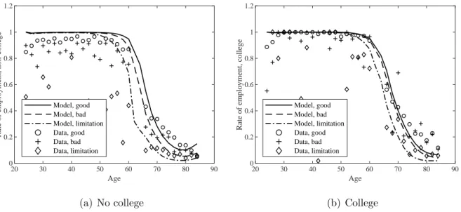
Figure 3 shows the model’s ability to reproduce life-cycle trends in employment across education and health groups. Consistent with data, in the model individuals without a Bachelor’s degree retire earlier than individuals with a Bachelor’s degree, and individuals with bad health or work limitations retire earlier than individuals with good health.
Assets and OAI claims: Figure 4 shows median assets by age, revealing a good fit.
Despite low earnings at young ages, individuals start saving very early in their careers in order to accumulate precautionary savings (Low, 2005). In the model, assets increase
20 30 40 50 60 70 80 90 Age 0 0.1 0.2 0.3 0.4 0.5 0.6 0.7 0.8 0.9 1 Rate of employment Model Data (a) Employment 20 30 40 50 60 70 80 90 Age 0 0.05 0.1 0.15 0.2 0.25 0.3 0.35 0.4 Total Hour Model Data (b) Hours
Figure 2: Employment Rates and Total Hours by Age
Source: Employment data from the MEPS and HRS. Hours data from the PSID and
HRS. 20 30 40 50 60 70 80 90 Age 0 0.2 0.4 0.6 0.8 1 1.2
Rate of employment, non-college
Model, good Model, bad Model, limitation Data, good Data, bad Data, limitation (a) No college 20 30 40 50 60 70 80 90 Age 0 0.2 0.4 0.6 0.8 1 1.2
Rate of employment, college
Model, good Model, bad Model, limitation Data, good Data, bad Data, limitation (b) College
Figure 3: Employment Rates by Age, Health and Education
Source: Employment data from the MEPS and HRS.
until people reach their early 60s; as people start to retire, they spend down their assets and wait for the optimal time to claim OAI benefits. Asset levels increase between age
70 and 84, and are almost unchanged after age 85. Three mechanisms account for the slow asset decumulation after retirement: the bequest motive, precautionary savings for longevity risks, and the need to pay for medical expenses, especially nursing home costs.
20 30 40 50 60 70 80 90 100 Age 0 0.5 1 1.5 2 2.5 3 3.5 Median assets 105 Model Data
Figure 4: Median Assets by Age
Note: Asset data from the 2013 SCF.
Figure 5 displays OAI recipiency rates.14 Although the model does not target these
rates, Figure 5(a) shows that it matches the general claiming patterns. The model un-derstates age-62 claiming in 2012 by about 17 percentage points (pp). This may be due to the absence within the model of illiquid housing wealth.15 If individuals who wish to retire early have few liquid assets, they may need to claim their Social Security benefits at younger ages (c.f., Kahn 1988; Kaplan and Violante 2014). Illiquid housing may also explain why assets in the data do not dip when people are in their early 60s. Figure 5(b) shows that within the model people without a college degree are more likely to claim early, consistent with their shorter lifespans. It bears noting that Figure 5 does not account for DI. By age 62, about 16% of the population is on DI, most of them without a college degree.
14In the model, as in actual practice, DI beneficiaries are transferred to OAI at age 66.
15Pashchenko and Porapakkarm. (2018), who study claiming in some detail, find it to be sensitive to
In recent years there has been an ongoing trend toward later claiming, even though people born between 1943 and 1954 – the cohorts making retirement decisions in our anal-ysis – face the same NRA and claiming adjustments. In addition to the claiming decisions observed in 2012, Figure 5(a) shows claiming in 2016, which more closely resembles the model’s predictions. 62 63 64 65 66 67 68 Age 0 0.1 0.2 0.3 0.4 0.5 0.6 0.7 0.8 0.9 1
Rate of OAI Recipiency
Model Data, 2012 Data, 2016
(a) Aggregated, data and model
62 63 64 65 66 67 68 Age 0 0.1 0.2 0.3 0.4 0.5 0.6 0.7 0.8 0.9 1
Rate of OAI Recipiency
Non-college College
(b) Disaggregated, model
Figure 5: OAI Recipiency Rates by Age, Education and Health
Note: The claiming rate for the data is computed as the age-by-age ratio of male retired worker beneficiaries for 2012 (year-end) from the SSA Statistical Supplement (Social Security Administration 2014, Table 5.A1.1) to the estimated male population (United States Census Bureau 2019a, average of July 2012 and July 2013, and July 2016 and July 2017). In panel (b), solid series are for individuals without a Bachelor’s degree, and dashed series are for individuals with a Bachelor’s degree.
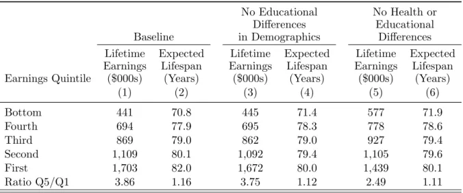
Income and Lifespan Heterogeneity: Table 2 shows, for three model
specifica-tions, mean lifetime earnings (discounted at an annual rate of 5%) and life expectancy for each lifetime earnings quintile. The first two columns show results for the baseline model. Individuals in the top earnings quintile earn nearly 4 times as much as those in bottom quintile, and they live 11 years longer. By way of comparison, (Chetty et al., 2016, Figure 3) found that in 2015, the age-40 life expectancy of men in the bottom household income quartile was about 10 years lower than that of men in the top quartile.
The difference for women was 6 years. Noting that we condition on lifetime, rather than current, earnings, our mortality gradient is arguably similar to Chetty et al.’s (2016).
Table 2: Earnings and Expected Lifespan by Lifetime Earnings Quintile
No Educational No Health or Differences Educational Baseline in Demographics Differences Lifetime Expected Lifetime Expected Lifetime Expected Earnings Lifespan Earnings Lifespan Earnings Lifespan Earnings Quintile ($000s) (Years) ($000s) (Years) ($000s) (Years)
(1) (2) (3) (4) (5) (6) Bottom 441 70.8 445 71.4 577 71.9 Fourth 694 77.9 695 78.3 778 78.6 Third 869 79.0 862 79.0 927 79.4 Second 1,109 80.1 1,092 79.4 1,105 79.6 First 1,703 82.0 1,672 80.0 1,439 80.1 Ratio Q5/Q1 3.86 1.16 3.75 1.12 2.49 1.11
4
Welfare Maximizing Policies
We turn to finding the policies that maximize aggregate welfare, which we define as the ex-ante lifetime utility of a newborn. We search over 5 parameters: the payroll tax cap yss; the parameters ss
1, ss2 and ss3 of the benefit function ssb(E) (see
equa-tion (13)); and the curvature parameter A of the claiming adjustment function Abk (see
equation (14)). However, we require the welfare maximizing policy to generate the same aggregate expenditures – to do this we adjust all benefits proportionally – as the baseline policies, eliminating a degree of freedom. Because our goal is to maximize welfare while holding Social Security’s aggregate footprint fixed, we also adjust payroll taxes so that the reformed system collects the same revenues as the baseline policies. We assume that changes in the payroll tax rate (2·∆τss) and the payroll tax cap (yss) apply only to workers
We maintain general government budget balance by changing the tax parameter λ0,
holding public goods (G) fixed. We fix DI benefits at their benchmark levels as well. Although interactions between OAI and DI are undoubtedly important, in our model DI claiming is treated as exogenous. We include DI recipiency to ensure that our analysis of OAI reforms is not driven by disability-related outcomes; we do not analyze DI itself.
4.1
Benchmark environment
Column (1) of Table 3 summarizes the optimal policies for our benchmark environment. The optimal policies have three important features: (1) the cap on taxable earnings changes only modestly; (2) the PIA does not depend on average lifetime earnings; (3) the adjustments for early or late claiming are smaller than the current adjustments.
Cap on taxable earnings (yss). The first line of Table 3 shows that the optimal
cap on taxable earnings equals 197% of median AIME, roughly the current level (see column (0)). Raising the upper bound on taxable earnings has two main effects. The first is that a larger tax base leads to a lower payroll tax rate (Figure 6(a)), increasing employment among both the college and non-college educated (Figure 6(b)). The second is that it raises the marginal tax rate for workers with earnings near the previous cap. These are among the most-skilled workers in the economy. Figure 6(c) show that average earnings (over all individuals) generally fall as the tax cap rises. Even as employment increases, the decrease in labor supply among the most-skilled is enough to reduce average earnings. The effect is most pronounced among the college-educated.
Figure 6(a) shows that increasing the cap leads to lower bequests. The increased employment associated with the lower payroll tax rate leads workers to claim their Social Security benefits at older ages. Retirees receive higher annual benefits, reducing the wealth they carry into very old ages. Given that SS expenditures are held fixed, it is not surprising that the median benefit available to age-66 claimers – the median PIA
Table 3: Current and Optimal Policies in Stationary Equilibrium
Current Demographics 2050 Demographics Current Optimal 1 Optimal 2 Current Optimal 1 Optimal 2 Benefit Taxation and
Yes Yes No Yes Yes No
Earnings Test
(0) (1) (2) (3) (4) (5)
Tax cap / median
2.18 1.97 2.03 2.18 3.09 3.10
age-62 AIME
Age-66 benefit (PIA) percentiles (000s)
10th percentile 30.7 43.6 42.8 21.0 33.9 34.4
median 42.1 43.7 43.2 28.9 33.9 34.8
90th percentile 55.1 43.9 43.7 37.8 33.9 35.1
Benefits relative to age-66 benefit
age 62 0.74 0.78 0.80 0.74 0.81 0.80 age 70 1.32 1.26 1.23 1.33 1.22 1.23 Benefit claiming age 62 6.0% 30.7% 81.5% 1.8% 26.8% 85.4% age 66 66.0% 100.0% 100.0% 36.8% 99.8% 100.0% Employment age 62 69.6% 64.1% 66.6% 74.4% 69.4% 72.7% age 70 24.8% 21.5% 25.6% 38.4% 37.8% 40.7% Aggregate behavior employed 76.4% 75.1% 75.9% 73.4% 72.3% 73.1% hours—employed 0.33 0.33 0.33 0.33 0.33 0.33 earnings ($000s) 87.7 86.7 87.4 97.1 95.9 96.5 assets ($000s) 123.3 129.3 133.8 200.5 205.2 208.8 bequests ($000s) 6.1 6.4 6.8 10.5 10.7 11.2 consumption ($000s) 73.5 72.9 74.1 87.1 86.3 87.3 τss 6.2% 6.5% 6.8% 5.0% 4.8% 5.5% λ0 25.8% 25.9% 25.5% 25.8% 26.1% 25.8%
Residual government budget (000s)
revenues 23.6 23.6 23.6 28.5 28.5 28.5
expenses 3.3 3.3 3.3 4.2 4.2 4.2
balance 20.3 20.3 20.3 24.3 24.3 24.3
Internal (annual) rate of return on OAI and DI
all households 1.15% 1.15% 1.15% 0.48% 0.48% 0.48%
no college degree 1.61% 1.96% 1.91% 0.94% 1.81% 1.69% college degree 0.54% -0.12% -0.06% 0.25% -0.31% -0.25% Consumption equivalent variation
all households 1.16% 2.31% 1.50% 2.22%
no college degree 1.38% 2.57% 1.98% 2.76%
– changes little.16 The small differences that do appear are due to changes in claiming
patterns and changes in the maximum benefit, which is tied to the cap: to maintain the expenditure target, these necessitate small changes in PIA levels.
The final panel of Figure 6 shows welfare effects, which we measure as the ex-ante con-sumption equivalent variation (CEV), the proportional increase in lifetime concon-sumption needed to make a newborn individual in the benchmark economy as well off as a newborn in the counterfactual economy.17 Because we construct Figure 6 using the optimal values
of ssb(E) and Abk, the CEV, which is relative to the current Social Security policies, is
generally positive. Although expanding the cap from its benchmark level reduces aggre-gate earnings, most households benefit from the lower payroll tax rate. Low values of the taxable limit thus lead to significant welfare losses. This dynamic reverses once the cap reaches its optimal value, although the losses from setting the cap above its optimal value are small.
PIA formula (ssb(E)). Returning to Table 3, column (1) shows that the optimal PIA
function is flat in lifetime earnings. This is a radical departure from current U.S. rules, where individuals at the 90th percentile of the PIA distribution receive 70% more than those at the 10th percentile, but not unprecedented internationally. As B¨orsch-Supan et al. (2016, Table 1) document, although most countries include an earnings-related component in their public pensions, a non-trivial number provide only a basic benefit.
As with any form of worker compensation, changing the PIA formula generates both income and substitution effects. Figure 7 provides more detail. Although the PIA depends on three parameters (subject to an expenditure constraint), to simplify the discussion Figure 7 characterizes policies with a single variable, the 90-10 benefit ratio. Higher values of this dispersion ratio correspond to a stronger positive relationship between earnings and
16Because we account for earnings test credits in our simulations by modifying AIME (E
j), we calculate
this hypothetical benefit using age-62 AIME.
17We calculate this as lifetime utilityreform−utility from bequestsbenchmark
lifetime utilitybenchmark−utility from bequestsbenchmark
1/[γ(1−σ)]
−1, with all utility measured ex-ante.
0 1 2 3 4 5
Cap/median age-62 AIME
0.9 1 1.1 1.2 1.3 1.4 1.5 1.6 Ratio to benchmark Benchmark OPT Bequest transfers Median PIA Employee tax rate Income tax rate
(a) Equilibrium variables
0 1 2 3 4 5
Cap/median age-62 AIME
0.72 0.73 0.74 0.75 0.76 0.77 0.78 0.79 0.8 Employment rate Benchmark OPT All NC C (b) Employment rate 0 1 2 3 4 5
Cap/median age-62 AIME
0.975 0.98 0.985 0.99 0.995 1 1.005 Earnings/Benchmark Benchmark OPT AllNC C (c) Earnings 0 1 2 3 4 5
Cap/median age-62 AIME
-1.5 -1 -0.5 0 0.5 1 1.5 CEV % Benchmark OPT All NC C (d) CEV %
Figure 6: Effects of changing the limit on taxable earnings
benefits. Figure 7(c) shows that tying the PIA more tightly to AIME increases aggregate earnings. Holding total benefits fixed, a steeper earnings gradient causes benefits for non-college workers to fall. This income effect, which encourages work, is reinforced by the substitution effect from tying benefits to earnings. Employment and earnings both rise monotonically in the 90-10 ratio. For college-educated workers, the income effect of
1 1.5 2 2.5 3 90-10 benefit ratio 0.95 0.96 0.97 0.98 0.99 1 1.01 1.02 1.03 1.04 1.05 Ratio to benchmark Benchmark OPT Bequest transfers Median PIA Employee tax rate Income tax rate
(a) Equilibrium variables
1 1.5 2 2.5 3 90-10 benefit ratio 0.73 0.74 0.75 0.76 0.77 0.78 0.79 0.8 Employment rate Benchmark OPT All NC C (b) Employment rate 1 1.5 2 2.5 3 90-10 benefit ratio 0.975 0.98 0.985 0.99 0.995 1 1.005 1.01 Earnings/Benchmark Benchmark OPT All NC C (c) Earnings 1 1.5 2 2.5 3 90-10 benefit ratio -0.2 0 0.2 0.4 0.6 0.8 1 1.2 1.4 CEV % Benchmark OPT AllNC C (d) CEV %
Figure 7: Effects of changing the PIA formula
linking benefits to earnings is negative, at least for high earners, and both employment and income fall (Figure 7(b)). The increase in non-college earnings is steeper, however, and these workers constitute the majority of the labor force. Aggregate earnings rise.
Figure 7(a) shows that the relationship between benefit dispersion and bequests is U-shaped. Tying benefits more closely to earnings reduces the need of richer households to save, reducing bequests, which by construction are luxury goods. On the other hand,
higher values of the 90-10 ratio also result in higher benefits for the rich, and thus higher wealth. Around the benchmark value of the 90-10 ratio, the second effect starts to domi-nate the first, and bequests begin to rise.
Figure 7(d) shows that, labor supply notwithstanding, the welfare effects of changing the PIA formula are driven by redistribution. As the 90-10 ratio increases, benefits are moved from less-educated to more-educated workers, lowering the welfare of the first group and raising the welfare of the second. Within education groups, there is also redistribution between individuals with different wage and health histories. Overall, moving from the current PIA function to a flat one raises the CEV by 0.7%.
Figure 7(d) also shows that that welfare is increasing even as the benefit formula becomes completely flat. Allowing the benefits to decrease in lifetime earnings would increase welfare even further. This is because the tax and transfer system as a whole is not sufficiently redistributive. Given that we examine only part of this system, we view a flat Social Security benefit formula as a natural lower bound for our exercise.
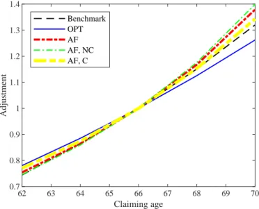
62 63 64 65 66 67 68 69 70 Claiming age 0.7 0.8 0.9 1 1.1 1.2 1.3 1.4 Adjustment Benchmark OPT AF AF, NC AF, C
Figure 8: Claiming age adjustments
and optimal (solid blue line) benefit adjustments for early or late claiming, relative to benefits at the NRA. The figure also shows the actuarially fair adjustments, based on the model’s mortality rates and a post-tax interest rate of 3% per year. Comparing slopes reveals that under the current rules, the Social Security adjustments are more or less actuarially fair prior to the NRA, but less than fair post-NRA.
In Figure 9(a), median age-66 benefits are plotted against the size of the claiming adjustment, measured as the ratio of age-70 to age-62 benefits. Two mechanisms are in play. First, larger claiming adjustments will induce delayed claiming. This can raise or lower aggregate expenditures, depending on the sizes of the adjustments. Second, holding claiming dates fixed, larger adjustments will reduce expenditures on early claimers and raise expenditures on those who claim late. Figure 9(a) shows that when the claiming adjustments are small, and most individuals claim early, increasing the claiming adjust-ment generates cost savings and thus higher benchmark PIA levels. In this region of the policy space, larger claiming adjustments raise annual benefits for late claimers not only directly but also indirectly, through higher values of the PIA. As adjustments continue to grow the expenditure effects reverse, and base benefits fall.
Figure 9 also shows that as claiming adjustments increase, and more workers delay claiming, employment and earnings both rise. Figure 9(a) shows that payroll taxes fall until the 70-62 benefit ratio reaches 1.6. After this point, delayed claiming reduces Social Security-related income taxes to such an extent that payroll taxes have to be increased. Higher earnings initially lead bequests to rise, but as the adjustments grow and workers claim at increasingly later dates, they increasingly rely on their Social Security benefits.
The welfare effects of the claiming adjustments are driven both by their direct effects on benefits and on their induced effects on labor supply. Larger claiming adjustments initially lead to higher statutory benefits and significantly higher earnings, increasing welfare. As adjustments continue to rise, their effect on the PIA reverses, earnings growth diminishes, and benefits shift from the short-lived (low earners) to the long-lived. The CEV begins to
1 1.2 1.4 1.6 1.8 2 2.2 70 to 62 benefit ratio 0.8 0.85 0.9 0.95 1 1.05 1.1 Ratio to benchmark Benchmark OPT Bequest transfers Median PIA Employee tax rate Income tax rate
(a) Equilibrium variables
1 1.2 1.4 1.6 1.8 2 2.2 70 to 62 benefit ratio 0.72 0.73 0.74 0.75 0.76 0.77 0.78 0.79 0.8 Employment rate Benchmark OPT All NC C (b) Employment rate 1 1.2 1.4 1.6 1.8 2 2.2 70 to 62 benefit ratio 0.95 0.96 0.97 0.98 0.99 1 1.01 Earnings/Benchmark Benchmark OPT All NC C (c) Earnings 1 1.2 1.4 1.6 1.8 2 2.2 70 to 62 benefit ratio -1.5 -1 -0.5 0 0.5 1 1.5 CEV % Benchmark OPT All NC C (d) CEV %
Figure 9: Effects of changing the claiming age adjustments
fall. Moving from the optimal claiming adjustment to the one currently in place reduces CEV by about 0.5%.
Discussion. Relative to the policies currently in place, the optimal Social Security
policies reduce work incentives in order to redistribute resources from high to low earners. Benefits are disconnected from earnings; and the rewards to delayed claiming (and longer careers) are reduced; only the payroll tax is relatively unchanged. Comparing the first
two columns of Table 3 shows that under the optimal policies, the number of people claiming benefits at age 62 rises by 25 pp. The aggregate employment rate declines by 1.7% and average earnings decline by 1.1%. Receiving smaller benefits, high-earnings workers save and bequeath more, raising aggregate bequests. Consumption declines by 0.8%. Nonetheless there is a CEV gain of 1.16%. The gain goes entirely to those without college degrees; the college-educated experience a loss of about -0.06%.
To quantify the extent to which Social Security redistributes resources, we calculate internal rates of return on Social Security benefits and taxes for the college- and non college-educated. Column (0) of Table 3 shows that the existing system is already fairly redistributive, with annual returns of 1.61% and 0.54%, a difference of 1.1 pp, for those without and with college degrees, respectively. Our estimates contrast with Goda et al. (2011) who calculate returns using Social Security earnings histories. They find rates of return to be moderately progressive (i.e., decreasing in lifetime earnings) for women and slightly regressive for men. (Our mortality rates apply to both sexes.) A major reason for the difference is that our model accounts for benefit taxation and DI. Removing these two elements causes our estimated rate of return for the non college-educated to fall to 0.87% and our estimated rate for the college-educated to rise to 0.62%. Our results differ more from S´anchez-Romero et al.’s (2019) estimates for men born in 1960, which are fairly regressive, with rates of return for the 2nd and 4th income quintiles of 1.1pp and 2.4pp, respectively (Table 4, case DB-II). It seems unlikely that the differences are due solely to the modelling of Social Security benefits, as the ratio between the top and bottom quintiles of lifetime Social Security benefits reported by S´anchez-Romero et al. (2019, Figure 2), 1.8, is similar to our 90-10 ratio for the PIA, 1.79. DI and benefit taxation again account for some of the difference.
In any event, the optimal Social Security rules described in column (1) are far more redistributive than the current rules. The rate of return for those without a college degree is 2.1 pp higher than the rate for those with a degree, which is in fact negative. It is
notable that under our optimal policies the less-educated earn a higher rate of return despite our utilitarian welfare criterion. A utilitarian social planner, seeking to equate marginal utilities among the living, will naturally place more weight on the long-lived.
A handful of papers have examined the effects of changing the progressivity of the Social Security benefit formula, employing a range of modelling assumptions and reaching a variety of conclusions. Using a model where there are no earnings-mortality links of any sort, Nishiyama and Smetters (2008) conclude that benefits should be increasing more rapidly in earnings than under current rules, arguing that the distortions associated with a progressive benefit formula outweigh the gains from risk-sharing. Huggett and Parra (2010), in contrast, find that benefits should bedecreasing in lifetime earnings. While they also treat earnings and mortality as independent, their analysis differs from Nishiyama and Smetters (2008) in terms of equilibrium concept and household composition, in both cases being more similar to ours. On the other hand, Ndiaye (2018), whose model differs from Huggett and Parra’s (2010) primarily in having a retirement decision, reaches the same general conclusion as Nishiyama and Smetters (2008). Ndiaye (2018) also finds that the claiming adjustments should be amplified; we discuss this finding in the robustness section below.
Bagchi (2019) develops a model where mortality depends on earnings. He also finds that the optimal benefit formula is one that is less redistributive, i.e., has benefits more closely tied to earnings, than the current rules. One potential reason why Bagchi’s (2019) finding differs from ours is the assumption of endogenous mortality. In his framework labor supply decisions affect length of life, while in our framework exogenous differences in health and education, which affect mortality, also affect earnings. As Hall and Jones (2007) show, spending on longevity affects lifetime utility in ways fundamentally different from that of spending on consumption. Bagchi and Jung (2019) find that when mortality is exogenous but tied to health, the optimal benefit is independent of earnings; in an earlier version of Bagchi (2019) where mortality depends on wealth, Bagchi (2016) finds
a flat benefit to be optimal. Bagchi’s papers differ from our model in other ways: they all impose closed-economy equilibrium, while we hold wages and interest rates fixed; we consider claiming decisions, the earnings test, and benefit taxation, while they do not.
4.2
Benchmark environment, no earnings test or benefit
taxa-tion
Because the amount of Social Security benefits subject to income taxation increases in total income, the income taxation of these benefits can significantly raise the marginal tax rate on earnings, discouraging individuals from simultaneously working and receiving benefits. This dynamic, along with the earnings test, implies that claiming decisions are in part retirement decisions. Jones and Li (2018) showed that, under the existing benefit formula, eliminating both the earnings test and benefit taxation increases labor supply and welfare. We now introduce these reforms, increasing the payroll tax to maintain budget balance, and solve again for optimal policies. Column (2) of Table 3 shows the results. Column (2) shows that the optimal taxation limit, benefit formula and claim-ing adjustments are more or less independent of the earnclaim-ings test or benefit taxation. Eliminating the latter two provisions, however, generates significant increases in employ-ment, earnings, consumption and welfare. Over half of the employment loss generated by the reforms in column (1) is offset by the reforms in column (2), as is 70% of the earnings loss. Consumption actually rises relative to its baseline value. The combined reforms considered in column (2) allow Social Security to be more redistributive than at present, while imposing fewer distortions than in column (1). Notably, college- as well as non-college-educated workers benefit from the joint reforms.
Removing the earnings test and the income taxation of benefits uncouples the claiming and labor supply decisions. As we move from column (0) to column (1), the increase in age-62 claiming, from 6.0% to 30.7%, is accompanied by a fall in age-62 employment,