Regional variations of 1932–34 famine losses in Ukraine
Oleh Wolowyna
1Serhii Plokhy
Nataliia Levchuk
Omelian Rudnytskyi
Alla Kovbasiuk
Pavlo Shevchuk
AbstractYearly estimates of urban and rural direct losses (excess deaths) from the 1932–34 famine are presented for the oblasts of Soviet Ukraine. Contrary to expectations, the highest losses are not found in the grain-producing southern oblasts, but in the north-central Kyiv and Kharkiv oblasts. Several hypotheses are proposed and tested to explain this finding. No single hypothesis provides a comprehensive explanation. Losses in some oblasts are due to specific factors, while losses in other oblasts seem to be explained by a combination of economic and political factors. Quantitative analyses are presented of resistance and Soviet repressions in 1932, and effects of the food assistance program and historical-political factors on direct losses in 1933 are analyzed.
Keywords: 1932–33 famine losses by oblast; Holodomor; regional Holodomor losses; Ukrainian famine; urban and rural Holodomor losses.
Résumé
Des estimations annuelles de pertes (décès excédentaires) directement attribuables à la famine de 1932–34 sont présentées pour les zones urbaines et rurales d’Ukraine sovietique. Contrairement aux attentes, les pertes les plus importantes n’étaient pas dans la région méridionale productrice de grain, mais plutôt dans la région du nord-centre, soit Kiev et Kharkiv. Plusieurs hypothèses sont proposées et mises à l’épreuve pour vérifier cette conclusion. Cependant, aucune hypothèse, à elle seule, ne fournit une explication complète. Dans certaines régions, les pertes sont causées par des facteurs précis, alors que dans d’autres, les pertes sont expliquées par une combinaison de facteurs économiques et politiques. Des analyses quantitatives sont présentées sur la résistance et les répressions sovietiques en 1932. L’effet du programme d’assistance alimen-taire et les facteurs politico-historiques attribuables directement aux pertes en 1933 est également analysé.
Mots-clés : pertes de la famine de 1932–33 par région; holodomor; pertes régionales de l’holodomor; famine en Ukraine; pertes urbaines et rurales de l’holodomor.
Introduction
The 1932–34 famine in Ukraine, also known as the Holodomor (death by hunger), is an extreme example of a man-made famine that resulted in millions of losses.2 As a result of our research, Holodomor losses have been
estimated at 4.5 million, with 3.9 million excess deaths and 0.6 million lost births (Rudnytskyi et al. 2015). Direct losses or excess deaths (these terms will be used interchangeably) are additional deaths caused by the famine; indirect
1. Oleh Wolowyna, Center for Slavic, Eurasian and East European Studies, University of North Carolina at Chapel Hill, 935 White Cross Rd., Chapel Hill, NC 27516 USA, e-mail: [email protected]; Serhii Plokhy, Director, Harvard Ukrainian Research Institute; and Nataliia Levchuk, Omelian Rudnytskyi, Senior Researchers, and Alla Kovbasiuk and Pavlo Shevchuk, Researchers, Ptoukha Institute of Demography and Social Studies, at the National Academy of Sciences of Ukraine (NASU), Kyiv.
losses or lost births are births that did not occur due to the famine, i.e., they would have occurred had there been no famine. In this article, we present estimates of yearly direct Holodomor losses by oblast for urban and rural areas, and propose explanations for the differences found.
While numerous studies have attempted to estimate Holodomor losses for Ukraine, estimates at the region-al level are scarce. S. Kulchytskyi (2003) and S. Maksudov (2012) anregion-alyzed mortregion-ality differentiregion-als at the oblast level, and Wheatcroft and Garnaut (2013) did the same at the raion level. However, these studies were based on registered deaths and did not attempt to estimate direct or indirect losses. Estimation of regional Holodomor losses is important for several reasons. First, it shows that the average national and urban-rural estimates hide significant regional differences. Second, it quantifies the losses in each region. Third, these data provide the demographic underpinnings necessary for historical analyses of the Holodomor and its consequences at the subnational level. Fourth, it helps us to better understand the dynamics of the Holodomor and its consequences.
The analysis presented here is based on our previous work on yearly estimates of direct Holodomor losses in Ukraine, by urban and rural areas and by age and sex (Rudnytskyi et al. 2015), and on a discussion of regional dif-ferences in direct Holodomor losses that is based on maps posted as part of ‘The Great Famine’ component of the Mapa: Digital Atlas of Ukraine program developed by the Harvard Ukrainian Research Institute (Plokhy 2016).
Oblast losses are presented without age and sex detail, mainly because estimates by age at the oblast level are based on relatively small numbers of registered deaths, which affects reliability. We provide a brief discussion of urban losses, but the emphasis is on rural losses. The dynamics of urban excess deaths are quite different from rural dynamics, and require a separate analysis. Estimates of oblast urban and rural losses are adjusted to the national urban and rural estimates presented in our previous work.
The loss estimates cover the administrative structure of Soviet Ukraine at the time of the famine, i.e., seven oblasts (Vinnytsia, Kyiv, Chernihiv, Kharkiv, Donetsk, Dnipropetrovsk, and Odesa), and also the Moldavian Autonomous Soviet Socialist Republic (ASSR). Our analysis shows distinct regional patterns in the spatial dis-tribution of the direct losses.
NOTE: The Moldavian ASSR is included in our analysis because it was part of the Ukrainian SSR during the famine period. It was separated from Soviet Ukraine in 1940 and was not a part of it thereafter. To simplify the presentation, in some cases we will refer in the text to ‘seven oblasts’ instead of ‘eight regions.’
Changes in administrative-territorial structure
Our estimation of losses is based on reconstruction of yearly populations for the eight regions of the Ukrainian SSR during the 1926–39 intercensal period. Several changes in the administrative structure during this interval had to be taken into account. The country was divided into 40 districts called okrugs 3 during the
1926–30 period; then the province-type oblasts were created to replace them, increasing progressively in number from 7 in 1932 to 15 in 1939. Also, an additional structure of six economic-geographical areas was in place dur-ing 1924–31 (Polissia, Right Bank, Left Bank, Dnipropetrovsk, Mountain Region, and Steppe). Furthermore, the country was divided into constantly fluctuating county-type raions during the whole 1926–39 period.
As all demographic data were recorded according to the administrative structure in place at the time of their collection, it was necessary to recalculate the data from different years to the seven-oblast-plus-Moldavia structure that was current during the 1932–34 famine period.
Recalculation of data into the seven-oblast structure
The seven oblasts of the Ukrainian SSR were in place between October 1932 and January 1937, and the territory of the Moldavian ASSR did not change during the 1926–39 period; thus, it was necessary for us to es-timate transition coefficients from the other administrative structures to the seven-oblast structure for the other years in the research period. These coefficients were applied in order to recalculate population by age and sex,
177
births, deaths, and migration data. In the end, specific transition coefficients were estimated for the following periods: 1926–28, 1929–31, 1937, 1938, and 1939.
1926–28: From 40 okrugs to seven oblasts
Our transition coefficients from 40 okrugs to seven oblasts are based on detailed maps for the above-men -tioned six economic areas that were published as part of the 1926 census. These maps show raion and okrug borders and allowed us to construct the oblasts based on these smaller units.
1929–31: From six economic-geographic zones to seven oblasts
Besides the normal tabulation by okrugs, the Central Statistical Administration of Soviet Ukraine (CSA UkrSSR) tabulated vital statistics by six economic-geographic areas during 1924–31. As vital statistics were not available by okrugs for the 1929–31 period—only for the six areas—our recalculation of vital statistics for this period was done in two steps: (1) estimation of transition coefficients from the six economic-geographical areas to the 40 okrugs; and (2) use of the transition coefficients estimated for the previous period, from the 40 okrugs to the seven oblasts.
The years 1937, 1938, and 1939
Two sets of transition coefficients were estimated for 1939: (1) for total populations—from 15 oblasts, as published for the 1939 census, to seven oblasts (Poliakov 1992; Korchak-Chepurkivskyi 1962); and (2) for populations by age and sex—from the 17-oblast structure in place in 1969 to seven oblasts (CSA USSR 1969). The first set of coefficients was used to estimate total populations for each oblast, yearly births, deaths by age and sex, and net migration. The second set of coefficients was used to estimate population by age and sex in 1939. Transition coefficients from 15 to seven oblasts were based on populations by raion that were published in the 1939 census. A similar methodology was used to estimate transition coefficients for 1937, from 11 to seven oblasts (five oblasts were subsequently added to the seven oblasts, on 22 September 1937), and for 1938 from 12 to seven oblasts. These coefficients were used to estimate population by age and sex for 1937, as well as births, deaths by age and sex, and net migration for 1937 and 1938.
Data and methods
Our reconstruction of the yearly demographic dynamics of the eight regions in the Ukrainian SSR for the 1926–39 intercensal period was based on the following data: 1926, 1937, and 1939 population censuses, 1931 urban count, rural-urban reclassification of population settlements, yearly numbers of births and deaths, and migration statistics.
Estimation of overall Holodomor losses was based on a detailed reconstruction of the yearly populations in the eight regions during the 1926–39 period. The actual population dynamics were calculated by making relevant adjustments to census data, vital statistics, estimations of migration, and urban-rural reclassifications; the yearly populations were then calculated based on these components.
Adjustments of the three Soviet censuses are described below. We also adjusted the official 1931 urban count for the Ukrainian SSR to compensate for the undercount of children aged 0–4 years (ANER 1933b). The undercount for urban areas was distributed proportionately to the respective populations in the eight regions. After all the adjustments were made, we shifted populations from the dates of the three censuses and the urban count to the closest January 1 date.
Adjustment of 1926, 1937, and 1939 censuses
The 1926 and 1937 censuses are considered to be of good quality; the 1939 census, on the other hand, was deliberately falsified to cover up the huge population losses due to the Holodomor and other repressive meas -ures revealed by the 1937 census (Andreev et al. 1990; Tolts 1995; Zhiromskaia 1990).Before using their data, we needed to make minor adjustments to the 1926 and 1937 censuses and major adjustments to the 1939 census. These corrections were applied to the official urban and rural population figures of the eight regions by sex and age, as published by the CSA USSR. The general methodology we used to make these adjustments is the same as the one we used in our previous work on Ukraine (Rudnytskyi et al. 2015); here we describe only the additional steps needed for adjustments at the regional level.
1926 census
We made two adjustments to the official 1926 census figures (CSA USSR 1929): redistribution of armed forces and adjustment of under-reporting for children aged 0–4 years. The census counted military personnel at the garrisons where they were stationed—mostly located in urban areas—thus introducing a significant distor -tion in the age structure of the urban popula-tion. We estimated the total number of armed forces sta-tioned in the Ukrainian SSR at 121,200, by applying the proportion of the civilian population in Ukraine to the total USSR civilian population, 19 per cent, to the total armed forces in the Soviet Union. This estimate was distributed in the eight regions, proportionately to their urban and rural populations.
Our adjustment of the undercount of children aged 0–4 years was done using a methodology developed by Korchak-Chepurkivskyi (1928) for Ukraine. Adjustment coefficients were estimated for each region and were applied to the urban and rural areas of the region. The overall average adjustment for Soviet Ukraine was 0.8 per cent, with the following breakdown for the eight regions: 1.3 per cent in Dnipropetrovsk and Odesa oblasts, 1.2 per cent in Moldavia, 1.0 per cent in Donetsk oblast, 0.8 per cent in Kyiv oblast, 0.6 per cent in Kharkiv and Vinnytsia oblasts, and 0.5 per cent in Chernihiv oblast.
1937 census
As stated in our paper on Ukraine (Rudnytskyi et al. 2015: 57):
The 1937 census was the first census conducted after the Great Famine, and it documented large population losses in Ukraine. It showed the total civilian population of Ukraine to be significantly lower than projected by central planners (the Central Economic Survey Administration of the USSR) and lower than in 1926. Given these unexpected results, the government declared the census ‘defective’ and its organizers were exe-cuted or exiled (Tsaplin 1989; Volkov 1990). Some of the 1937 census documents were destroyed, and the remaining results discredited because of supposedly flawed methods and organizational failures. Only in the late 1980s did the data from the 1937 census become available (Poliakov 1992), andit was shown that the census was executed correctly (Tolts 1989; Volkov 1990; Livshits 1990).
179
distribution among the eight regions was done using the same methods as for the 1926 census. Thus, the total number of armed forces in Ukraine in 1937 was estimated at 346,800, based on the proportion of the civilian population in Ukraine relative to the USSR total. The undercount of the 1937 census was estimated by Andreev et al. (1990) at 0.43 per cent for the whole Soviet Union. As we did not have elements for estimating undercount for Ukraine and its oblasts, the same percent was used for each oblast.
1939 census
It was discovered in 1990 that the 1939 census, considered for many years a model for Soviet censuses, was seriously flawed. A sophisticated falsification plan had been implemented to hide large population losses that were already documented in the 1937 census (Zhiromskaia 1990). Our adjustments to the census data at the regional level were made using the same methodology as the overall adjustments for Ukraine (Rudnytskyi et al. 2015). They included the elimination of two types of falsification: (1) inflated undercount and inflated adjust -ment factors for control forms; and (2) reassign-ment—to place of residence at time of census—of the census forms of persons in forced labour camps, “special groups,” and military personnel, which had been arbitrarily assigned to different parts of Ukraine.
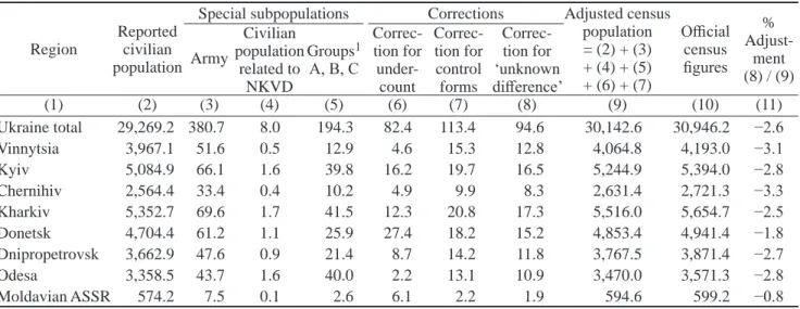
Table 1. Adjustment steps for 1939 census populations of Ukrainian SSR, by region (in 1,000s)
Region
Reported civilian population
Special subpopulations Corrections Adjusted census population = (2) + (3) + (4) + (5) + (6) + (7)
Official census figures % Adjust-ment (8) / (9) Army Civilian population related to NKVD Groups1 А, B, C
Correc-tion for under-count Correc-tion for control forms Correc-tion for ‘unknown difference’
(1) (2) (3) (4) (5) (6) (7) (8) (9) (10) (11)
Ukraine total 29,269.2 380.7 8.0 194.3 82.4 113.4 94.6 30,142.6 30,946.2 −2.6
Vinnytsia 3,967.1 51.6 0.5 12.9 4.6 15.3 12.8 4,064.8 4,193.0 −3.1
Kyiv 5,084.9 66.1 1.6 39.8 16.2 19.7 16.5 5,244.9 5,394.0 −2.8
Chernihiv 2,564.4 33.4 0.4 10.2 4.9 9.9 8.3 2,631.4 2,721.3 −3.3
Kharkiv 5,352.7 69.6 1.7 41.5 12.3 20.8 17.3 5,516.0 5,654.7 −2.5
Donetsk 4,704.4 61.2 1.1 25.9 27.4 18.2 15.2 4,853.4 4,941.4 −1.8
Dnipropetrovsk 3,662.9 47.6 0.9 21.4 8.7 14.2 11.8 3,767.5 3,871.4 −2.7
Odesa 3,358.5 43.7 1.6 40.0 2.2 13.1 10.9 3,470.0 3,571.3 −2.8
Moldavian ASSR 574.2 7.5 0.1 2.6 6.1 2.2 1.9 594.6 599.2 −0.8
1 A = NKVD; B = prisoners; C = forced resettlements
Sources: Poliakov (1991, 1992), Simchenko (1990), Kokurin and Petrov (2000), and authors’ calculations.
We redistributed the armed forces, estimated at 380,700 for the Ukrainian SSR, among the oblasts by rural and urban areas using the same methodology as in the 1926 and 1937 censuses. Next, data on “spe-cial groups”—NKVD personnel, prisoners, and forced settlers—were available only for the whole country (Poliakov 1992). However, the distribution of these special contingents by oblast and rural-urban areas was published in the 1937 census (Poliakov 1991), and we used these 1937 proportions to redistribute the total numbers of special contingents in Ukraine by oblast in 1939. Data on the civilian NKVD staff contingent, also available only for Soviet Ukraine overall, was distributed by oblast and rural-urban areas proportionately to the oblast distributions of the special contingents. Comparing our resulting adjusted figures with the offi -cial census figures, we arrived at an overall inflation factor for Ukraine of 2.6 per cent; at the oblast level, the inflation factors vary between 0.8 per cent for Moldavia to 3.3 per cent for Chernihiv oblast (see Rudnytskyi et al. 2015 for more details).
-mor (Simchenko 1990). As the official civilian population by age and sex contained these extra 383,600 prisoners residing outside Ukraine, we subtracted them from the rural populations of the five oblasts, using the age-sex structure of the labour camp populations (Kokurin and Petrov 2000).
Adjustment of vital statistics for under-registration
Registered numbers of births and deaths were distorted by different degrees of under-registration during the intercensal period; during the famine years, levels of under-registration reached extremely high proportions. The general adjustment approach used for urban and rural areas of Soviet Ukraine is described in Rudnytskyi et al. (2015), and the same approach was used for each of the eight regions. Only a brief conceptual description of the adjustment methodology is presented here.
We made adjustments along three dimensions: (1) crisis (1932–34) and non-crisis (1927–31 and 1935–39) periods; (2) urban, rural and total; and (3) three vital events: births, infant deaths, and deaths after one year of age. The adjustment methods for the three vital events differed, depending on the related dimension. Namely, the same adjustment methods were applied to the three events in urban areas during crisis and non-crisis per-iods, while different methods were applied (to the three vital events) during crisis years for rural and total popu-lations. In almost all cases, adjustments for rural areas were calculated as the difference between total and urban values. Ukrainian demographers did extensive research on this topic in the 1930s, and we took full advantage of their work in our adjustment methodology.
Estimation of net migration by oblast, 1927–38
Migration is difficult to estimate, as migration statistics are incomplete and fragmentary. Estimation of migration for urban areas is less problematic than for rural areas, as there was a migration registration system in place in cities during this period, while no such system existed in rural areas. In 1932 the urban registration system was improved by the introduction of registration cards for all arrivals and departures in most cities of Soviet Ukraine (Popov 1995). However, urban migration statistics are problematic, requiring systematic evalua-tion and adjustments for under-registraevalua-tion. Rural migraevalua-tion estimates had to be pieced together using different statistical sources and archival documents. Once the yearly rural and urban migration was estimated for each region, the respective totals were adjusted to the yearly net migration data for urban and rural areas of the Ukrainian SSR (Rudnytskyi et al. 2015).
Urban migration
The following data sources were used for estimating urban migration by oblast: (1) numbers of net migrants for Ukraine, 12 separate oblasts and the Moldavian ASSR for 1927–38, compiled by ANER without sex, age, and flow details (RSAE 1562/20/73); and (2) number of migrants by arrivals and departures, as well as net migrants, during 1933–38, by sex and age for all urban centers in each oblast (RSAE 1562/20/30, 38, 75, 75, 18, 145). We also had migration data for 1932 by arrivals and departures by sex, age and migration flows (RSAE 1562/20/27). The yearly numbers of net migrants, calculated by ANER for the 1927–38 period and for 12 oblasts, were recalculated by us for the seven oblasts using the appropriate transition coefficients. We then used these estimates of net migrants as the basis for estimating yearly numbers of urban migrants.
Our estimation of numbers of net urban migrants in each oblast was done for three separate periods, 1927–30, 1931–36, 1937–38, using the same method as for urban Ukraine (Rudnytskyi et al. 2015). Yearly disaggregation of the net migrants was done proportionately to the yearly number of registered net migrants. Thus, the total number of net urban migrants for the 1927–38 period is 3,792,200 (see Table 2).
181 Rural migration
We classified rural migration into two types of streams: internal and external. The main internal stream is rural-to-urban migration for the 1927–38 period. According to the urban registration system, of the total net urban migration about 81 per cent were rural-to-urban migrants, i.e., 3,085,800. We did a yearly distribution of this total according to the yearly distribution of rural-to-urban migrants in the urban registry system. Then, within each year we distributed the number of migrants among the oblasts proportionately to their rural population size.
The second internal stream is organized inter-oblast migration from rural to rural areas during 1934–35. Data on these migration streams can be found in Iefimenko (2013) and Iukhnovskyi et al. (2008). In 1934, 16,200 fam -ilies were resettled from Vinnytsia, Kyiv, and Chernihiv oblasts to Odesa, Kharkiv, Donetsk, and Dnipropetro-vsk oblasts; in 1935, 9,800 families were resettled from Vinnytsia and Kyiv oblasts to Donetsk, DnipropetroDnipropetro-vsk, and Kharkiv oblasts.
External rural migration is composed of nine streams, seven out-migration and two in-migration streams: 1. Persons sent to labour camps (gulags) and working colonies, 1929–38. Sources for these data are: Nikolskyi 2001;
Mozokhin nd; Zemskov 2005; and Tronko et al. 1994–2011; the total number of prisoners is 284,600. Detailed information on this type of emigration by oblast is available for 1937 and 1938; about 90 per cent of these migrants were males (Golotik and Minaev 2004). The 64,300 sent to penal camps in 1937–38 were distributed by oblast as follows: 24,200 in Vinnytsia, 10,700 in Kyiv, 8,200 in Donetsk, 6,300 in Kharkiv, 5,700 in Odesa, 5,200 in Dnipropetrovsk, 2,600 in Chernihiv, and 1,400 in Moldavia. For the other years, 1929–36, reliable statistics are available only for Ukraine, and yearly estimates for Ukraine were calculated in Rudnytskyi et al. (2015). These yearly numbers of migrants were distributed by oblast using the proportions available for 1937–38.
2. Eviction of kulaks,4 1930–33.Data on this migration stream can be found in: SARF 9414/1/1943, 1944; SARF 9479/1/2; Yakovlev et al. 2005; and Bugai 2013; the total number of evicted kulaks is 364,500. Detailed information on this migration is available for 1930 by 40 okrugs, and we recalculated the data for the seven oblasts. The 111,400 kulaks evicted in 1930 are distributed by oblast as follows: 24,400 in Odesa, 19,600 in Kharkiv, 18,100 each in Vinnytsia and Kyiv oblasts, 17,500 in Dnipropetrovsk, 7,200 in Donetsk, 3,600 in Chernihiv, and 3,100 in Moldavia. Total numbers for 1931, 1932, and 1933 were only available for Ukraine, and we redistributed them by oblast using the proportions from 1930. The yearly totals of evicted kulaks were 194,100 in 1931, 15,000 in 1932, and 44,000 in 1933.
3. Forced emigration of peasants, 1929–33.Statistics on this migration category are fragmentary and unreliable, as most of it took place during the Holodomor (RSAE 1562/20/22, 29, 30, 73; Vynnychenko 1994). The estimate is 532,200; yearly estimates were taken from Rudnytskyi et al. (2015), and numbers by oblast were distributed proportionately to the respective rural populations.
4. Organized mass resettlements of peasants, 1927–30. These resettlements were a continuation of previous campaigns to resettle peasants from Soviet Ukraine to Siberia and the Far East. A total of 120,000 were resettled in 1927–30 (Hirshfeld 1930; Platunov 1976; Rybakovskii 1990). The yearly overall numbers of migrants for Ukraine were distributed by oblast proportionately to their rural population.
5. Deportation of Poles and Germans to Kazakhstan in 1936. From areas in Vinnytsia and Kyiv oblasts bordering Polish-occupied Galicia and Volhynia, 14,900 peasant families (or 60,000 persons) were deported in 1936 to Kazakhstan (Yakovlev et al. 2005; Bugai 2013; Iefimenko 2013). We distributed this number by oblast proportionately to their rural populations.
6. Emigration of Jews, 1929–38.An ethno-demographic balance methodology was used by Rudnytskyi et al. (2015) to estimate the number of Jews who emigrated from Ukraine during this period. The number of 4. The Russian term kulak has entered English usage and is therefore used here in roman type and pluralized accordingly.
Jewish emigrants thus estimated for the intercensal period was distributed yearly, based on information from the following sources: Hirshfeld 1930; Weitsblit 1930; Vynnychenko 1994; Leskova 2005; Rudnik 2006. Approximately 57,000 Jews emigrated from Ukraine during this period, and this number was distributed among the oblasts, proportionately to the number of Jews in each oblast.
7. Peasants hired to work on construction projects in other parts of the Soviet Union, 1935–38. Information about this migration stream is fragmentary (Kozin 1936; Vynnychenko 1994; RSAE 1562/20/73, 75, 76, 118, 143, 145). According to our calculations, about 170,500 peasants from Vinnytsia, Kyiv, Chernihiv, and Odesa oblasts, as well as Moldavia, were involved in this state-run initiative. The yearly estimates calculated in Rudnytskyi et al. (2015) were distributed proportionately to the rural population of the oblasts and Moldavian ASSR.
8. Resettlement of peasants from Belarus and Russia to Ukraine during 1933–34. The 1932–34 famine left many villages in Ukraine practically empty, and the Soviet government decided to settle these villages with peasants from Belarus and Russia. Sources on these resettlements are: Iefimenko (2013) and CSANO (1/2/6583–85, 6392). During the second half of 1933 a total of 27,100 families (137,800 persons) were resettled from Belarus and from the following four regions of the RSFSR: Gorky (Nizhnii Novgorod) Krai and Yaroslavl, Western, and Central Black Earth oblasts. They were resettled in the following oblasts of the UkrSSR: 44,300 in Kharkiv, 39,600 in Dnipropetrovsk, 34,600 in Odesa, and 19,300 in Donetsk. However, a portion of these settlements turned out to be temporary; Iefimenko presents data that by March 1935, at least half of the settlement populations had left (2013: 143–48).
9. Resettlement of kulaks from Central Asia to Ukraine in 1931. The policy of destroying kulaks as a class was not limited to the European regions of the Soviet Union; it also affected wealthy farmers in Central Asia. More than 40 villages in Odesa oblast were recipients of peasants from Uzbekistan branded as kulaks (Vynnychenko 1994; Smolii et al. 2003; Zemskov 2005). According to our calculations, this contingent had about three thousand families (16,000 persons).
Our team systematized, evaluated, analyzed, and organized all these data into yearly numbers of net migrants by rural area in each oblast, resulting in −4,400,300 total net rural migrants. Net rural migration for the 1927–38 period was negative for all oblasts. Dnipropetrovsk oblast had the largest net migration, with −1,017,300. Add -ing net urban and rural migration, we obtained −608,100 net migrants for Ukraine (Table 2).
More detailed information discovered about urban-rural reclassification during our oblast estimates resulted in some changes in our total urban and rural net migration numbers compared to previous estimates for Ukraine (Levchuk et al. 2015; Rudnytskyi et al. 2015). The previous number of 4,108,000 net urban migrants changed to 3,792,200, and the previous number of −4,826,400 net rural migrants changed to −4,400,300. There were also minor adjustments to total number of deaths, from 8,519,600 to 8,640,100 in rural areas, and from 1,650,000 to 1,639,400 in urban areas, with a total of 10,279,500 deaths in Soviet Ukraine. These adjustments resulted in minor changes to the yearly balances of urban and rural areas by oblast. As a result of these changes, the number of direct losses for urban areas decreased by 2 per cent, and the number of direct losses for rural areas increased by 0.2 per cent; the total number of direct losses remained the same.
Population reconstruction by oblast, 1927–39
183
Table 2. Total population balance for Ukrainian SSR and its region, by urban-rural areas, 1927–38 (in 1,000s) A – Total
Region Population on
1 Jan. 1927 Births Deaths
Net migration
Population on 1 Jan. 1939
% annual natural rate
% annual total rate
Ukraine total 29,316.3 11,685.0 10,279.5 −608.1 30,113.8 0.42 0.22
Vinnytsia 4,405.1 1,678.2 1,542.7 −486.3 4,054.3 0.29 −0.69
Kyiv 5,877.6 2,182.0 2,328.8 −495.4 5,235.4 −0.17 −0.96
Chernihiv 2,812.6 1,010.8 850.3 −339.6 2,633.5 0.49 −0.55
Kharkiv 5,784.4 2,074.7 2,195.0 −159.2 5,504.9 −0.14 −0.41
Donetsk 3,007.5 1,746.8 1,128.6 1,221.1 4,846.9 1.57 3.98
Dnipropetrovsk 3,548.9 1,509.6 1,077.8 −203.2 3,777.6 0.98 0.52
Odesa 3,302.7 1,220.4 950.9 −103.1 3,469.1 0.68 0.41
Moldavian ASSR 577.5 262.5 205.4 −42.4 592.2 0.82 0.21
B – Urban
Region Population on
1 Jan. 1927 Births Deaths
Net migration
Urban–rural
reclassification Population on 1 Jan. 1939
% annual natural rate
Ukraine total 5,322.4 2,463.2 1,639.4 3,792.2 1,103.6 11,041.8 1.20
Vinnytsia 537.2 154.7 104.4 −28.9 −18.8 539.2 0.75
Kyiv 1,065.5 321.2 250.1 376.8 2.2 1,515.1 0.54
Chernihiv 344.5 101.0 75.7 215.9 −138.9 447.0 0.59
Kharkiv 981.5 357.2 261.8 585.6 238.4 1,900.8 0.77
Donetsk 942.8 889.3 521.1 1,498.2 760.6 3,570.7 2.75
Dnipropetrovsk 573.4 357.8 210.5 814.1 204.8 1,740.5 1.91
Odesa 797.8 251.8 198.5 328.3 27.3 1,206.3 0.54
Moldavian ASSR 79.6 30.1 17.3 2.1 27.9 122.3 1.24
C – Rural
Region Population on
1 Jan. 1927 Births Deaths
Net migration
Urban-rural
reclassification Population on 1 Jan. 1939
% annual natural rate
Ukraine total 23,994.0 9,221.8 8,640.1 −4,400.3 −1,103.6 19,071.8 0.20
Vinnytsia 3,867.9 1,523.5 1,438.2 −457.5 18.8 3,514.4 0.18
Kyiv 4,812.1 1,860.8 2,078.7 −872.2 −2.2 3,719.7 −0.39
Chernihiv 2,468.1 909.8 774.6 −555.5 138.9 2,186.6 0.44
Kharkiv 4,802.9 1,717.5 1,933.2 −744.8 −238.4 3,604.1 −0.38
Donetsk 2,064.8 857.5 607.6 −277.1 −760.6 1,277.0 0.95
Dnipropetrovsk 2,975.6 1,151.8 867.3 −1,017.3 −204.8 2,037.9 0.76
Odesa 2,504.8 968.6 752.4 −431.4 −27.3 2,262.3 0.69
Moldavian ASSR 497.9 232.4 188.1 −44.5 −27.9 469.8 0.71
In 1930 the CSA UkrSSR approved a new classification of urban settlements, with significant differences compared to the classification used for the 1926 census. In most oblasts, many urban settlements were reclassi -fied as rural settlements. Criteria used in this reclassification were: small population size and high percentage of the population in agriculturally related occupations. Donetsk and Dnipropetrovsk oblasts were the exceptions to this pattern, where many rural settlements were reclassified as urban settlements. The net result of rural-urban reclassifications in 1930 was an increase in the rural population by 194,100.
Final reconstructed total populations of the eight regions for 1927 and 1939 are presented in Table 2. During the intercensal period, the Ukrainian SSR had an overall annual average natural exponential growth rate (births minus deaths) of 0.4 per cent. Two oblasts, Kyiv and Kharkiv, lost population, while the other oblasts had an annual average natural growth rate of less than one per cent, except Donetsk, with a yearly rate of 1.6 per cent.
The urban population of Ukraine grew at an annual average natural growth rate of 1.2 per cent, and urban areas in all oblasts had positive growth. Donetsk had the highest annual average natural growth rate, with 2.7 per cent, followed by Dnipropetrovsk oblast with 1.9 per cent and Moldavia with 1.2. For the other oblasts, rates varied between 0.5 and 0.8 per cent. The average annual natural rate of growth for all rural areas was only 0.2 per cent, and Kyiv and Kharkiv oblasts had negative yearly natural growth of −0.4 per cent each. For all the other oblasts, the yearly natural rate of growth was positive, albeit quite small.
Direct Holodomor losses
Direct losses are estimated as the difference between the number of deaths occurring during the famine years, and the hypothetical number of deaths had there been no famine during the same period. We estimated the number of hypothetical deaths had there been no famine using linearly extrapolated age-specific deaths rates between 1931 and 1935, i.e., years before and after the famine, at a time when mortality was considered ‘normal.’
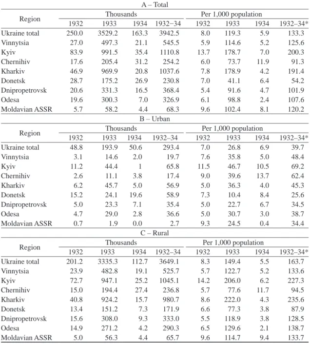
Our results for direct losses by oblast are presented in Table 3 in three panels: total, urban, and rural. The total number of direct losses for Ukraine is estimated at 3.9 million, with 250,000 in 1932, 3,529,000 in 1933, and 163,000 in 1934 (panel A). Most of the losses occurred in 1933 in all oblasts. In five oblasts, 90 per cent or more of the losses occurred in 1933, and the percentages for Donetsk and Chernihiv oblasts and Moldavia are 76, 81, and 85, respectively.
Kyiv oblast had the highest number of losses with 1,111,000, followed by Kharkiv with 1,038,000 and Vinnytsia with 546,000. Direct losses for Chernihiv, Donetsk, Dnipropetrovsk, and Odesa oblasts vary between 254,000 and 368,000, and Moldavia has the smallest number of direct losses, 68,000.
As the number of losses is directly related to population size, to make valid comparisons among oblasts it is necessary to control for population size. Focusing first on 1933, the total number of excess deaths for Soviet Ukraine in 1933 is 119 deaths per 1,000 population. Kyiv and Kharkiv oblasts have the highest losses, with 179 excess deaths per 1,000 population each, followed by Vinnytsia oblast with 115 and Moldavia with 102; Donetsk oblast has the lowest value, 41 direct losses per 1,000 population. The relative number of losses for Ukraine was lower in 1934 than in 1932, and this is the case for all except Chernihiv oblast, where relative losses were higher in 1934 than in 1932.
The ratios in the last column provide a summary of relative losses for the three famine years, calculated as the total number of losses for the three years, divided by the 1933 mid-year population and multiplied by 1,000. If we divide this indicator by 10, it can be used as an approximation of the per cent of the 1933 population that died due to famine. Thus, we can say that the total number of excess deaths constituted about 13 per cent of the 1933 UkrSSR population; Kyiv oblast had the highest value with 20 per cent, and Donetsk oblast had the lowest with 5 per cent.
The total urban excess deaths in Soviet Ukraine were 293,000, with 49,000 in 1932, 194,000 in 1933 and 51,000 in 1934 (Table 3, panel B); 66 per cent of all urban excess deaths occurred in 1933. Regarding excess deaths per 1,000 population, the yearly ratios are 7.0, 26.8, and 6.9 respectively, and almost 40 for the 1932–34 period.The concentration of urban direct losses in 1933 varies from around 80 per cent in Kharkiv and Odesa oblasts to 41 per cent in Donetsk oblast.
185
Discussion
This section is based on the discussion of regional differences of Holodomor direct losses posted on the website Mapa: Digital Atlas of Ukraine (Plokhy 2016). We systematized and quantified arguments presented in that paper, and elaborated the discussion with new elements.
As indicated above, the Holodomor dynamic in urban areas is very different from the one in rural areas and requires a separate, more detailed analysis. We present here a brief discussion of the urban losses, and then proceed to analyze in detail the spatial distribution of the rural direct losses.
Spatial distribution of excess deaths in urban areas
Research on the Holodomor has focused mainly on rural areas; our research shows that urban areas were also significantly affected by this famine. Relative 1932–34 direct losses represent 6.9 per cent and 6.2 per cent
Table 3. Direct losses (excess deaths) from the Holodomor in Ukrainian SSR, in numbers and by 1,000 population, by region and rural-urban areas
A – Total
Region Thousands Per 1,000 population
1932 1933 1934 1932−34 1932 1933 1934 1932–34*
Ukraine total 250.0 3529.2 163.3 3942.5 8.0 119.3 5.9 133.3
Vinnytsia 27.0 497.3 21.1 545.5 5.9 114.6 5.2 125.6
Kyiv 83.9 991.5 35.4 1110.8 13.7 178.7 7.0 200.3
Chernihiv 17.6 205.4 31.2 254.2 6.0 73.7 11.9 91.3
Kharkiv 46.9 969.9 20.8 1037.6 7.8 178.9 4.2 191.4
Donetsk 28.7 175.2 26.9 230.8 7.0 41.1 6.4 54.2
Dnipropetrovsk 20.6 331.3 16.5 368.4 5.4 91.6 4.7 101.9
Odesa 19.6 300.3 7.0 326.9 6.1 98.8 2.4 107.6
Moldavian ASSR 5.7 58.2 4.4 68.3 9.6 102.4 8.1 120.2
B – Urban
Region Thousands Per 1,000 population
1932 1933 1934 1932–34 1932 1933 1934 1932–34*
Ukraine total 48.8 193.9 50.6 293.4 7.0 26.8 6.9 39.7
Vinnytsia 3.1 14.6 2.0 19.7 7.6 35.8 5.0 48.4
Kyiv 11.2 44.4 1 65.8 11.5 46.7 10.5 69.2
Chernihiv 2.6 11.1 3.8 17.4 9.0 39.6 13.7 62.4
Kharkiv 6.2 45.7 5.0 56.9 5.0 36.3 4.0 45.3
Donetsk 15.2 24.1 19.6 58.9 7.3 10.4 8.4 25.6
Dnipropetrovsk 5.0 23.3 7.1 35.4 5.0 22.7 6.7 34.5
Odesa 4.7 29.0 2.8 36.6 5.0 30.7 3.0 38.7
Moldavian ASSR 0.7 1.9 0.0 2.7 9.3 24.5 0.4 34.4
C – Rural
Region Thousands Per 1,000 population
1932 1933 1934 1932–34 1932 1933 1934 1932–34*
Ukraine total 201.2 3335.3 112.7 3649.1 8.3 149.4 5.5 163.7
Vinnytsia 23.9 482.8 19.1 525.7 5.7 122.7 5.2 133.6
Kyiv 72.7 947.1 25.2 1045.1 14.2 206.0 6.2 227.3
Chernihiv 15.0 194.4 27.4 236.8 5.7 77.6 11.7 94.5
Kharkiv 40.8 924.2 15.7 980.7 8.6 222.0 4.3 235.6
Donetsk 13.4 151.2 7.3 171.9 6.6 77.3 3.8 87.9
Dnipropetrovsk 15.6 308.0 9.3 333.0 5.5 118.9 3.8 128.5
Odesa 14.9 271.2 4.2 290.3 6.5 129.6 2.1 138.7
Moldavian ASSR 5.0 56.3 4.4 65.7 9.6 114.7 9.4 133.7
of the urban populations in Kyiv and Chernihiv oblasts, respectively, while in the other oblasts they vary be-tween 2.6 per cent in Donetsk and 4.5 per cent in Vinnytsia oblasts (Table 3).
Rural losses are expected to be always higher than urban losses. However, we see that urban losses are higher than rural losses in 1934, namely, 6.9 and 5.5 per 1,000 persons, respectively. This surprising result can be ex-plained by considering the systemic relationship between urban and rural areas during the Holodomor.
As a result of the Soviet government’s policy to control agricultural production through the collectivization of farms, the state assumed direct responsibility for providing food to the urban population. Due to increasing shortages of food in cities, in 1931 the Politburo approved the resolution ‘On the introduction of a single sys-tem of supply for the working population by ration books.’ Key elements this resolution and its consequences are described as follows (emphasis added):
Only those who worked in the state sector of the economy (industrial factories, state and military organiza-tions and departments, and state farms) and their families received ration cards. Peasants and the politically disenfranchised were left out of the state food supply system. These people made up more than 80 per cent of the total population. Even ration sizes depended on how important people were to the industrialization process… From the beginning of 1931 there were four types of rations throughout the country: special, first, second, and third. They were called city lists, but in reality they were groupings of enterprises and organizations, because factories in the same city could be on different supply lists. The special and first lists had priority and included key industries in Moscow, Leningrad, Baku, the Donbas, Karaganda, Eastern Siberia, the Far East, and the Urals. Constituting only 40 per cent of the total number of people on rations, they received nearly 80 per cent of all the food supplies. The second and third lists included smaller and non-industrial cities’ (Osokina 2001: 61–62).
The ration system was affected by two opposite processes during the famine years: a rapid increase of the urban population triggered by Stalin’s industrialization policy, and diminishing food production due to peasant opposition to collectivization and increasing mismanagement of the agricultural sector (Levchuk et al. 2015). The result was a gradual diminishing of the official food ration amounts, especially on the lower ration lists; thus, an increasing proportion of the urban population ended up without any food assistance. By 1934, starva-tion reached critical levels in many cities, resulting in higher relative excess deaths in urban than in rural areas.
Spatial distribution of excess deaths in rural areas
In this section we discuss different factors that may explain the variable and unexpected regional distribu-tion of direct losses caused by the Holodomor, as shown in Map 1.
We start by presenting four hypotheses that have been suggested for the expected distribution of losses. Next, as the number of excess deaths experienced a drastic change between 1932 and 1933, we first examine factors related to the onset of the famine and regional distribution of direct losses in 1932. At the end of 1932, the north-central oblasts of the Ukrainian SSR had lower levels of collectivization and higher levels of grain quota fulfillment than the southern oblasts. This apparent contradiction leads us to examine, in the third sec -tion, the resistance to collectivization and grain procurement, and the repression of this resistance by the Soviet government. The explosion of excess deaths during the first half of 1933, and its relationship with the food ‘assistance’ program, are examined in the fourth section.
Four hypotheses
Several hypotheses have been suggested to explain the spatial variation in levels of excess deaths in rural areas of Ukraine: historical, ecological, border, and economic.
Historical hypothesis. The 1921–23 famine affected the southern grain-growing regions of Ukraine, and it was natural to assume that the 1932–34 famine would also have a more pronounced effect on these regions (Plokhy 2016: 378). As can be seen on Map 1, this was not the case for the 1932–34 famine; the highest losses are found in the north-central oblasts of Kyiv and Kharkiv.
187
in the north and steppes in the south. According to the ecological hypothesis, the expectation is that the relative number of excess deaths should be lowest in the Polissia zone and highest in the steppe zone. The rationale is that once most of the grain, and in many cases all food, was confiscated by the Soviet government, people in Polissia could find some food in the forests and swamps, while no alternative food was to be found in the steppe zone. Losses in the forest-steppe zone are expected to be in the middle range.
59 Map 1. Number of rural excess deaths per 100 population by oblast, Ukrainian SSR, 1932–34.
188
Unfortunately, the seven-oblast administrative structure of the Ukrainian SSR at that time does not provide a clear picture of the situation in the ecological zones, as they cut across oblast borders. However, detailed vital statistics available for 1933 allow us to estimate excess deaths at the raion level for that year, and Map 2 provides the resulting details. It is clear from this map that the ecological hypothesis does not explain the regional varia-tions in levels of excess deaths, as the highest relative direct losses are mainly in the forest-steppe zone, not in the steppe zone.
Border hypothesis. Map 2 also shows that the relative number of direct losses becomes lower the closer one gets to the international borders of Kyiv, Vinnytsia, and Moldavia with Poland and Romania. This pattern is consistent with the border hypothesis formulated by Shlyakhter (ch. 10, p. 1–2):
Exploring some of the striking regional variations in the famine’s severity, this paper argues that these dif-ferences resulted from a combination of official policies and the survival strategies of border strip inhabit -ants… In addition to offering an explanation for the lower mortality in Ukraine’s border districts during the Holodomor, this analysis also views the famine as a window onto Soviet security and revealshowcasing policies in the border strip, peasant survival strategies, and the interplay between the two.
Economic hypothesis. Given the failure of the ecological hypothesis to explain the spatial variations in excess deaths, Plokhy (2016: 379) suggests that ‘on the eve and in the course of the Great Ukrainian Famine, environ-mental factors influenced human actions, particularly government policies that eventually contributed to the death toll.’ Specifically, Moscow focused its attention on the grain-producing areas of southern Ukraine, as they had the optimal capacity to produce the grain needed for the implementation of Stalin’s policies, while other regions were left basically to their own devices.
189
Map 3 shows the distribution of wheat growing areas in 1937, and it can be used as an approximation of grain growing areas in 1932–34. Major grain growing areas are located in Odesa, Dnipropetrovsk, and Donetsk oblasts and Moldavia, while only 10 per cent of Chernihiv oblast is dedicated to grain crops. The agriculture of Kyiv, Kharkiv, and Vinnytsia oblasts is more diversified, with sugar beet, potatoes, and legumes besides grains. Thus, the policy of favouring the southern oblasts makes economic sense.
In a situation of generalized agricultural crisis like the one in 1932 (see discussion below), decisions had to be made about the priorities of resources, and Moscow’s more favourable treatment of the grain-producing oblasts was expected to result in lower relative direct losses in these oblasts than in the rest of the Ukrainian SSR. Comparing Maps 1 and 3, we see that this is only partially true. Although in general the southern oblasts have lower relative losses than the northern oblasts, there are exceptions. In the steppe zone, Donetsk oblast has significantly lower relative direct losses than Dnipropetrovsk, Odesa, and Moldavia. In the forest-steppe zone, Vinnytsia oblast has much lower losses than Kyiv and Kharkiv oblasts, and the level of its losses is similar to that of most oblasts in the steppe zone. Chernihiv oblast also does not conform to the economic hypothesis, as its relative direct loss is as low as in Donetsk oblast.
1932: Early manifestations of the Famine
To better understand the reasons for the differences in relative direct losses among the different oblasts, it is necessary to examine separately what happened in 1932 and 1933, as the dynamics of the Holodomor changed drastically between 1932 and 1933.
Regional differences in rural direct losses were already present in 1932. Kyiv oblast had the highest number of excess deaths per 1,000 population, with 14.2, followed by Moldavia with 9.6 and Kharkiv with 8.6; losses in the other oblasts vary between 5.5 and 6.6 excess deaths per 1,000 population (Table 3). Some of the reasons for this situation are described in detail in a letter to Stalin from the head of the Council of People’s Commissars of the Ukrainian SSR, Vlas Chubar, in June 1932, which is quoted by Plokhy (2016: 382):
The failure of legume and spring crops in those raions, above all, was not taken into account, and the insuffi -ciency of those crops was made up with foodstuffs to fulfill the grain requisition plans. Given the overall im -possibility of fulfilling the grain requisition plan, the basic reason for which was the lesser harvest in Ukraine as a whole and the colossal losses incurred during the harvest (a result of weak economic organization of the collective farms and their utterly inadequate management from the raions and from the center), a system was put in place of confiscating all grain produced by individual farmers, including seed stocks, and almost complete confiscation of all produce from the collective farms… In addition to grain procurements, the same methods were applied to potato and, especially, meat procurements.
The situation in Kharkiv oblast was no better. After his tour of Kharkiv oblast, Hryhorii Petrovsky, head of the Communist Party’s Central Executive Committee for the UkrSSR, wrote to Stalin in June 1932 that ‘famine has engulfed a good part of the countryside… It will take a month or a month and a half for new grain to appear… This means that famine will intensify’ (Plokhy 2016: 383). In a list of raions most affected by the famine, compiled by Party officials in Kharkiv in June 1932, Kyiv and Vinnytsia oblasts had 10 and 11 raions, respectively, while the number of affected raions in the southern oblasts was much smaller. The critical situa-tion in Kyiv and Kharkiv in 1932 is confirmed by the high relative direct losses in these two oblasts;5 the lower
level in Vinnytsia oblast (an international border oblast) was likely due to the lower mortality in the border areas (border oblast).
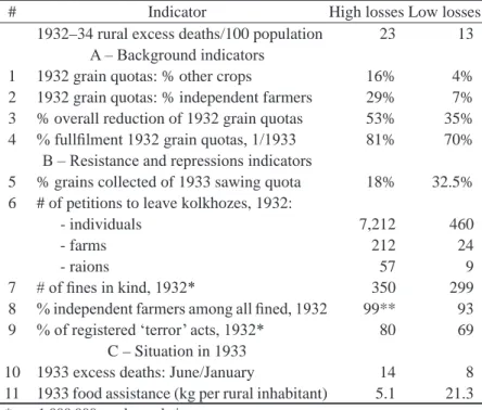
A key factor at the beginning of the famine was the grain procurement plan for 1932 (Table 4). It docu-ments the expectations of the Soviet government regarding Ukraine’s contribution to Stalin’s overall procure-ment plan, and provides a fairly good understanding of the conditions in the different oblasts. The total 1932 quota for the Ukrainian SSR was 5,831,000 tons of grain. This target seems reasonable, as it constituted 90 per cent of the amount collected from the 1931 crop. The relative allocation of this quota among the different
oblasts favoured the forest-steppe oblasts of Kyiv, Kharkiv, and Vinnytsia, at the expense of the steppe oblasts. Compared to what was collected in 1931, the amounts allocated to the steppe oblasts are higher than to the forest-steppe oblasts. The plan also takes into account the mixed-crop composition of the forest-steppe zone, with much higher allocations to these crops for the oblasts in this zone than for the oblasts in the steppe zone. It also acknowledges the fact that the proportion of independent farmers was much higher in the forest-steppe than in the steppe zone, and their grain quotas are much higher in the former than the latter.
The official procurement plan corroborates, at a more general level, Chubar’s impressions about the situation in Kyiv and Vinnytsia oblasts. It provides credence to Chubar’s statement that the unexpected failure of the non-grain crops and the heavy reliance of the official non-grain procurement plan on these crops had dire consequences. The crop failure led to widespread famine in the forest-steppe zone, forcing the government to confiscate most of the grain at kolkhozes and impose even harsher confiscation measures on individual farmers.
The extreme famine conditions in many areas of the forest-steppe zone, and to a lesser degree in the steppe zone, forced the Ukrainian SSR government in Kharkiv 6 to petition repeatedly for some relief from the grain
procurement quotas. After strong resistance, Stalin had to accept reality, and grain procurement quotas were re-duced three times during 1932: two significant reductions in August and October, and a more modest reduction at the end of the year.
Table 5. Successive reductions of 1932 grain quotas for Ukrainian SSR, by region Original quota % reduction January 1933 quota
Region million poods
% distr.
August 1932
October 1932
January 1933
million poods
% overall reduction
% distr.
Ukraine total 356 100 11 25 29 210 41 100
Vinnytsia 39 11 23 12 0 26.5 32 13
Kyiv 31 9 35 30 0 14 54 7
Kharkiv 74 21 11 41 3.4 35.5 52 17
Dnipropetrovsk 88 25 4.5 20 12 55.5 37 26
Odesa 84 24 2.3 17 12 56 33 27
Donetsk 36 10 14 33 2 19 47 9
Moldavian ASSR 4 1 12 22 0 3 29 1
Note: Chernihiv oblast was created later in 1932. Source: Pyrih 2007: 242, 298, 303–04, 355–56, 601–02.
The first round of reductions favoured heavily the forest-steppe zone at the expense of the steppe zone. Kyiv oblast received the largest reduction, with 35 per cent, followed by Vinnytsia oblast with 23 per cent and
Table 4. Grain procurement quotas for Ukrainian SSR in 1932, by region 1932 grain procurement quotas
Region
1932 grain procurement quotas, % of 1931 quota
tons
% of other crops (non-grain and
forage)
% of quota for independent
farmers
Ukraine total 90.0 5,831,000 9.7 17.1
Vinnytsia 88.0 639,000 22.4 40.2
Kyiv 65.5 511,000 26.0 41.1
Kharkiv 74.5 1,212,000 11.9 23.8
Dnipropetrovsk 90.0 1,441,000 5.3 6.8
Odesa 140.0 1,376,000 1.7 6.7
Donetsk 95.0 583,000 7.4 5.1
Moldavian ASSR 46.0 69,000 2.9 30.4
191
Kharkiv with 11 per cent, while reductions for Odesa and Dnipropetrovsk oblasts were in the 2.3–4.5 per cent range. Donetsk oblast received a reduction of 14 per cent, significantly higher compared to the other two steppe oblasts; this was repeated also during the next round of reductions. (The special status of Donetsk oblast will be further discussed below.) During the second round of reductions, Kharkiv and Kyiv again received large reductions, which prompted the steppe oblasts to demand significant reductions as well.
Overall, the grain procurement quota for the Ukrainian SSR was reduced by 41 per cent. Kyiv and Kharkiv oblasts had their original quotas reduced by more than half, and Vinnytsia oblast by one-third. The reduction for Odesa and Dnipropetrovsk oblasts was about one-third, and for Donetsk oblast it was close to half.
Table 6. Percent fullfillment of grain quotas by region in Ukrainian SSR, as of 1 Jan. 1933
Region Kolkhozes Sovkhozes Independent
farmers Total
% collectivized as of 1 Oct. 1932
Ukraine total 78 86 72 77 69
Chernihiv 92 96 68 78 47
Vinnytsia 100 95 100 100 59
Kyiv 100 101 90 100 67
Kharkiv 85.5 92 44 77 72
Dnipropetrovsk 70 82 54 69.5 85
Odesa 73 70 57 72 84
Donetsk 76 77 85 76 84
Moldavian ASSR 89 40.5 108 93 68
Sources: Pyrih 2007: 571–72; ANER 1935: 205.
The grain quota fulfillment results and collectivization levels shown in Table 6 are surprising, if not puz -zling. By October 1932 the steppe oblasts had reached very high levels of collectivization, while levels of col-lectivization in the forest-steppe and Chernihiv oblasts were significantly lower. In contrast, by the end of 1932 Kyiv and Vinnytsia had fulfilled 100 per cent of the grain procurement quotas, and Kharkiv close to 80 per cent, while the average for the forest oblasts was around 75 per cent. The collectivization levels are consistent with the official objective of faster collectivization of the grain-producing steppe region. The grain quota fulfillment data merit a more detailed analysis.
Fulfillment data is available for three groups: kolkhoz, sovkhoz,7 and independent farmers. For the kolhozes and
sovkhozes, per cent fulfillment is similar for all oblasts within each zone; per cent fulfillment is higher among the forest-steppe zone oblasts than among the steppe zone oblasts. The differences between the forest-steppe and steppe oblasts are mainly due to the performance of the independent farmers. Although independent farmers fulfilled over half of their quotas in Dnipropetrovsk and Odesa, and 85 per cent in Donetsk, this had little impact on the overall quota, due to the small proportion of independent farmers in these oblasts. The low performance of Kharkiv oblast, on the other hand, is due exclusively to the very low output fulfillment per cent from the independent farmers.
Resistance and repressions in 1932
Why is it that in spite of their relatively lower level of collectivization, the forest-steppe oblasts of Soviet Ukraine, except the independent farmers in Kharkiv oblast, show such extraordinary levels of compliance with the grain requisition plan? One possible answer is that these oblasts had been granted substantial reductions in their grain quotas (Table 5). Another possibility is the ‘ruthless efficiency of the local Party machine in requi -sitioning grain from the peasantry’ in Kyiv and Kharkiv oblasts, as a reaction to active and passive resistance (Plokhy 2016: 389).
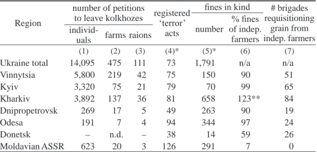
Table 7. Selected indicators of resistance and repression in Soviet Ukraine during the Holodomor, by region
Region
number of petitions
to leave kolkhozes registered‘terror’
acts
fines in kind # brigades requisitioning
grain from indep. farmers number
% fines
of indep. farmers individ-
uals farms raions
(1) (2) (3) (4)* (5)* (6) (7)
Ukraine total 14,095 475 111 73 1,791 n/a n/a
Vinnytsia 5,800 219 42 75 150 90 51
Kyiv 3,320 75 21 79 70 99 65
Kharkiv 3,892 137 36 81 658 123** 84
Dnipropetrovsk 269 17 5 49 263 90 19
Odesa 191 7 4 94 344 97 24
Donetsk – n.d. – 38 14 59 26
Moldavian ASSR 623 20 3 126 291 7 0
Notes: Chernihiv oblast is not listed as it was created in 1932 and some indicators are missing; * indicators standardized by size of oblast’s rural population; (1)…(3) June 1932;
(4) 1 Jan. 1932–31 Jan. 1933; (5)–(6) 5 Dec. 1932; (7) 5 Dec. 1932; ** error in original data
Source: Pyrih 2007: 250, 445, 456, 631.
The following factors of resistance and repression are quantified in Table 7: exodus from the kolkhozes, acts of ‘terror,’ total fines, including in kind and percentage of independent farmers fined, and number of Com -munist Party grain-search ‘brigades.’ The flight from kolkhozes was quite extensive in the forest-steppe oblasts, but negligible in the steppe oblasts. While the relative number (standardized by the rural population of each oblast) of registered acts of ‘terror’ was very high in Odesa oblast, on average this indicator was higher in the forest-steppe than in the steppe oblasts.
The picture regarding number of fines in kind, also standardized by the rural population in each oblast, is less clear-cut. This indicator was extremely high in Kharkiv oblast, quite low in Vinnytsia and Kyiv, and very low in Donetsk oblast. In all oblasts except Donetsk, the great majority of fines in kind were applied to independent farmers.
On 11 November 1932, the Central Committee of the Communist Party of the Ukrainian SSR ordered the creation by December 1 of at least 1,000 brigades to search for hidden grain among the independent farmers. The proposed number of brigades was much higher for the forest-steppe oblasts than for the steppe oblasts: 200, 300, and 350 for Vinnytsia, Kharkiv, and Kyiv oblasts, respectively, and 50 each for the three steppe oblasts; these proportions are maintained when the numbers are standardized by the rural population of each oblast. The higher number of brigades for the forest-steppe oblasts was due, in part, to the fact that these oblasts had more independent farmers. The very high percentage of grain procurement quotas for independent farmers in Vinnytsia and Kyiv oblasts (Table 4), and the fact that independent farmers in these oblasts had the highest percent fulfillment of these quotas (Table 6), tend to support the ‘ruthless efficiency’ argument.
Further evidence about the more aggressive grain requisition practices in Kyiv and Kharkiv oblasts during 1932 is provided in a report on the fulfillment of seed grain quotas for the 1933 harvest. As of 10 December 1932, only 20.5 per cent and 16.5 per cent of the quotas were filled in Kyiv and Kharkiv oblasts, respectively, while 40 per cent of the quota was filled in Dnipropetrovsk, 28 per cent in Donetsk, and 22 per cent in Ode -sa oblasts. These numbers support the hypothesis that most of the grain was already taken away in Kyiv and Kharkiv oblasts due to more aggressive requisition, while there was still a fair amount of grain left in the steppe oblasts. More updated data for Kharkiv oblast tends to confirm this hypothesis. Namely, it was reported that by 15 February 1933, only 35.6 per cent of the seed grain quota was fulfilled, and that the campaign was facing strong resistance (Pyrih 2007: 697).
193
oblasts were consequently subject to harsher repressions. The evidence may not be conclusive, as there is no certainty that the documents found so far are representative of the total picture in each oblast. Nevertheless, they show a correlation that is quite suggestive.
1933: Famine as terror
The number of relative rural losses presented in Map 1 is for the whole 1932–34 period. As 90 per cent of all losses occurred in 1933, the level of these losses is determined to a great extent by what happened in that year. In rural areas, two processes were happening in 1933: (1) extraordinary increase in monthly registered deaths during the first 6–7 months (Wolowyna 2013); and (2) implementation of a food aid program by Moscow as a reaction to this critical situation.
Between January and June 1933, the number of registered rural deaths increased by 11 times in Kyiv and Kharkiv oblasts, and eightfold in Vinnytsia oblast; in Odesa, Dnipropetrovsk, and Donetsk oblasts the in-creases ranged from fourfold to sevenfold, and in Moldavia rural registered deaths increased by half. These extraordinary increases were the result of several measures implemented by the Soviet government in late 1932 and early 1933.
First, two of these measures prevented peasants from travelling in search of food: (1) the introduction in December 1932 of domestic identity documents (“passports”) only for city residents, limiting the peasants’ abil-ity to travel to cities in search of food; and (2) the closing of borders between Ukraine (as well as the Northern Caucasus) and Russia in January 1933, stopping the flow of Ukrainian peasants to Russia in search of food. Thousands of Ukrainian peasants were arrested in Russia and returned to their villages (CC ACP 2001).
Second, Stalin’s directive dated 1 January 1933 reiterated the penalties outlined in the decree dated 7 August 1932, for ‘stealing’ stalks from the fields or hiding grain from the State, and harsh penalties in kind (meat and potatoes) introduced on 18 and 20 November 1932 for independent farmers and kolkhozes that did not fulfill their grain quotas.
Third, numerous brigades of Communist Party activists descended towards the end of 1932 and beginning of 1933 on villages to confiscate hidden grain, although most of it had been already seized, especially in Kyiv and Kharkiv oblasts. According to thousands of testimonies, even if no grain was found, in many instances every last scrap of food was confiscated (see also Chubar’s letter to Stalin above).
Fourth, a system of blacklists was instituted in November 1932 against kolkhozes, entire villages, and in some cases raions that failed to fulfill their grain quotas, and was gradually expanded to the whole country. ‘For a village to be blacklisted meant that: (1) all stores would be closed and supplies removed from the village; (2) all trade was prohibited, including trade in food or grain; (3) all loans and advances were called in, including grain advances; (4) the local Party and collective farm organizations were purged, and usually subject to arrest; (5) food and livestock would be confiscated as a ‘penalty’; and (6) the territory would be sealed off by OGPU (secret police) detachments’ (Andriewsky 2015). In other words, a death sentence was imposed on the population of the given kolkhoz, village, or raion.
Once Moscow realized the catastrophic nature of the famine, a program of food aid was implemented during the first half of 1933. The program entailed loans that the oblasts were required to pay back from the next harvest with 10 per cent interest, and had other strong restrictions. Boriak (2012) documents in detail the characteristics of this program: (1) the food was to be given mainly to members of kolkhozes who were willing and able to work, and to independent farmers willing to join the kolkhozes and work; (2) instructions for the administration of the program show clearly that its main objective was not to prevent starvation but to provide badly needed aid in order to save the next sowing season; (3) a good part of the food provided came from in-ternal reserves (in Ukraine), that had been requisitioned from Ukrainian farmers in 1932 and were now being given back to them as ‘assistance’, with selective distribution.
Dnipropetrovsk Odesa Kharkiv Kyiv Vinnytsia Donetsk Chernihiv Moldavia
tons food aid 56,200 49,400 29,900 19,900 9,600 3,300 1,200 300
kg per person 20.5 22.3 6.4 3.9 2.3 1.6 0.5 0.6
The data illustrate the importance of using relative indicators when making comparisons. In absolute num-bers, the bulk of the food aid went to Dnipropetrovsk and Odesa oblasts, with sizeable contributions also to Kharkiv and Kyiv oblasts. However, standardizing by the size of the respective rural populations introduces significant changes in the distribution. For example, the ranking between Dnipropetrovsk and Odesa oblasts is reversed, and more importantly, the difference in food aid amounts between Dnipropetrovsk and Odesa and the forest-steppe oblasts becomes much more pronounced. Thus, the actual amount to Dnipropetrovsk oblast is three times that given to Kharkiv oblast, instead of just under double as per the unadjusted figures.
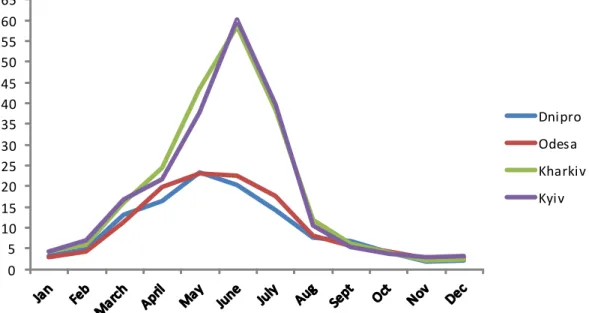
To illustrate the devastating effect of Stalin’s measures in late 1932 and early 1933 on the level and distribution of monthly losses in these oblasts in 1933, we selected two oblasts from the forest-steppe region, Kyiv and Khark-iv, and two from the steppe region, Odesa and Dnipropetrovsk. We show the relationship between the volume and timing of this food aid, and the number and monthly pattern of excess deaths in each of these oblasts.
The oblasts in the forest-steppe and those in the steppe region have very different patterns of monthly excess deaths in 1933 (Figure 1). Kyiv and Kharkiv experienced a sharp increase in monthly excess deaths between January and June, and then a sharp decrease. The rate of increase for Odesa and Dnipropetrovsk was somewhat smaller than for Kyiv and Kharkiv oblasts, with the peak in June being much lower and the decrease during the second half of 1933 being much less pronounced. The ratio of direct losses between the peak month of June and January of 1933 is even higher than the ratio of registered deaths. During the first half of 1933, the number of excess deaths increased by 14–15 times in Kharkiv and Kyiv, and by 7–8 times in Dnipropetrovsk and Odesa oblasts.
Figure 2 shows the timing and volume of food distributed to the different oblasts, in tons per 1,000 rural population. The graph shows very clearly that Odesa and Dnipropetrovsk oblasts received much more food aid than Kyiv and Kharkiv oblasts, and that this assistance started to arrive much earlier.
Comparing the two figures, we see a strong relationship between the food aid dynamics and the patterns of monthly excess deaths. The volume and timing of food distributed are clearly reflected in the two distinct patterns of monthly direct losses. The large amounts of food sent to Dnipropetrovsk and Odesa oblasts in February and March had two effects: it slowed down the monthly increase of direct losses and resulted in much lower peaks in June. The absence of practically any food aid to Kyiv oblast before March, or to Kharkiv oblast before April, resulted in faster rates of increase and much higher peaks in direct losses for these two oblasts.
One can also detect specific effects of the food assistance on the distribution of excess deaths in certain oblasts. For example, the rate of increase in monthly excess deaths slowed down between March and April in Kyiv oblast compared to Kharkiv oblast, and in Dnipropetrovsk oblast compared to Odesa oblast. This is likely related to the large amount of food aid sent to Kyiv oblast in mid-March, and larger amounts of food aid pro-vided to Dnipropetrovsk oblast than to Odesa oblast in February and March.
It is clear that the food aid program saved many lives in Odesa and Dnipropetrovsk oblasts. However, the main goal of the program was to save the 1933 harvest, and thus the assistance was targeted at specific oblasts and groups. As a result, many more peasants were condemned to death by starvation in Kyiv and Kharkiv ob-lasts than in the strategically more important obob-lasts of Odesa and Dnipropetrovsk. Although the number of excess deaths was significantly lower in the steppe than in the forest-steppe oblasts, the rate of monthly increase and maximum levels of death in Odesa and Dnipropetrovsk were still extremely high.
Historical legacy of peasant uprisings
195
and summer of 1919, which had forced them out of Ukraine, and in particular out of its two capitals (Kyiv and Kharkiv).8 This historical memory resulted, first, in stronger repressions and thus higher excess deaths in 1932,
and then in a decision, taken in late 1932 and applied during the following months, to use hunger as a tool to eradicate the possibility of a new general uprising, and to deprive the Ukrainian national movement of its social base, which Stalin had identified as being the villages (Graziosi 2015).
If this hypothesis is correct, the effects of the food aid program on 1933 direct losses, as described in the section ‘1933: Famine as terror,’ need to be compared to the effects of the punitive policy in the different re-gions. Testing this hypothesis requires two elements: a map depicting the historical revolts at the raion level, and
8. This may have been a factor in the decision, taken in 1929, not to discontinue the extant state indigenization program (korenizatsiia, or, in the case of the Ukrainian SSR, ukraїnizatsiia) during collectivization—precisely because of the awareness of the need to prevent a repetition of social and national elements combining to engender peasant revolts, as had occurred in Ukraine in 1919.
Figure 1. Monthly direct losses (per 1,000 rural population) for four oblasts of the Ukrainian SSR, 1933.
Source: Authors’ calculations. 0
5 10 15 20 25 30 35 40 45 50 55 60 65
Dnipro Odesa Kharkiv Kyiv
0 2 4 6 8 10 12 14 16 18 20 22 24 26
2/07 2/18 3/11 3/18 4/01 4/20 4/26 5/29 5/31 6/13 6/23 7/04 7/20
Dnipro Odesa Kharkiv Kyiv